Évaluation de l’influence de l’éclairement de croissance et de la température de surface des océans sur le rendement quantique de la fluorescence de la chlorophylle a induite par le soleil

Département de Géomatique Appliquée Faculté des lettres et sciences humaines

Université de Sherbrooke

TEL 804 Mémoire de maîtrise

Évaluation de l’influence de l’éclairement de croissance et de la température de surface des océans sur le rendement quantique de la fluorescence de la chlorophylle a induite par le

soleil

Marc-André Faucher

Table des matières

Résumé ... i

Remerciements ... ii

Avant proposs ... iii

Chapitre 1 : Introduction ...1 Objectifs ... 8 Hypothèses ... 8 Sites d’étude ... 8 Chapitre 2 : Article ...10 1. Introduction ...12

1.1. Assessing the global variations of 𝜑_𝑓𝑎𝑝𝑝 ... 15

2. Method ...19

2.1. Data sources ... 19

2.2. Growth irradiance algorithm ... 20

2.3. 𝜒𝑓𝑙𝑢𝑜 algorithm ... 23

3. Results ...24

3.1. Overview of data distribution ... 24

3.2. Modeling the 𝜒𝑓𝑙𝑢𝑜 vs 𝐸𝑔 relationship... 34

3.3. Simulating 𝜒𝑓𝑙𝑢𝑜 ... 35

4. Discussion ...37

4.1. Overall average of 𝜒𝑓𝑙𝑢𝑜 ... 37

4.2. 𝜒𝑓𝑙𝑢𝑜 vs SST ... 37

4.3. 𝜒𝑓𝑙𝑢𝑜 vs Eg ... 38

4.4. Comparison with other studies and potential sources of improvement ... 39

4.5. Noise in MODIS-Aqua’s measurement of fluorescence ... 41

5. Conclusion ...44

Chapitre 3 : Conclusion ...46 Références ...48

~ i ~

Résumé

Le phytoplancton, un ensemble de microorganismes photosynthétiques, est responsable de près de la moitié de la production primaire nette planétaire. Malgré son importance primordiale dans le cycle du carbone et du support de la vie marine, personne n'est encore en mesure d’expliquer la distribution du rendement quantique apparent de la fluorescence de la chlorophylle, un paramètre intimement lié à la physiologie et à l'état de santé de ces organismes. Dans le but d'apporter des précisions quant au comportement du rendement quantique apparent de la fluorescence de la chlorophylle à l'échelle des océans, nous avons évalué l'influence d’un ensemble de paramètres environnementaux notamment l'éclairement de croissance et la température de surface des océans sur le rendement quantique apparent de la fluorescence de la chlorophylle.

De plus, nous proposons une nouvelle façon de calculer l’éclairement de croissance à partir de l'éclairement photosynthétiquement utilisable (éclairement pondéré en fonction de l'absorption du phytoplancton), moyen entre la surface et la profondeur de la couche de mélange. L’éclairement photosynthétiquement utilisable est privilégié puisqu'il est plus représentatif que l'éclairement photosynthétiquement actif (éclairement total entre 400 et 700 nm) généralement utilisé dans le calcul de l’éclairement de croissance. Plutôt que de calculer le rendement quantique apparent de la fluorescence de la chlorophylle, ce qui est très complexe à faire de

façon exacte en raison de multiples paramètres difficilement évaluables, nous calculons le 𝜒𝑓𝑙𝑢𝑜,

un indice équivalent, mais qui a l’avantage de ne pas faire des suppositions sur certains paramètres physiologiques et écologiques.

Les résultats démontrent que le rendement quantique apparent de la fluorescence de la chlorophylle diminue quand l’éclairement de croissance augmente, ce qui suggère une augmentation de l’inhibition non photochimique de la fluorescence causée par une photoacclimation/photoadaptation du phytoplancton vivant dans un environnement d’éclairement important. Les résultats indiquent aussi que lorsque la température est sous 6°C l’impact sur le rendement quantique apparent de la fluorescence de la chlorophylle est significatif. Sous cette température, un groupe de pixels a été identifié pour lesquels le rendement quantique apparent de la fluorescence de la chlorophylle est essentiellement constant à des valeurs faibles. Ceci peut

~ ii ~

potentiellement pointer vers un plus large phénomène écosystémique/de communauté. Des simulations effectuées à partir d’une table de référence à trois dimensions (i.e., éclairement de croissance, température de surface des océans et concentration de chlorophylle) démontrent l’impact de ces paramètres sur le rendement quantique apparent de la fluorescence de la chlorophylle. Le modèle a répliqué avec succès certaines zones de fort et de faible rendement. Les divergences entre les données simulées et observées indiquent probablement la présence d’autres processus physiologiques indépendants de la température et de l’éclairement de croissance.

Remerciements

Je n’aurais sans doute pu réaliser ce travail seul. J’aimerais donc remercier tous ceux qui y ont contribués de près ou de loin, à commencer par mon directeur de maîtrise, le professeur Yannick Huot. D’abord pour sa confiance dans mes capacités à mener le projet à terme, mais aussi pour le financement du projet, pour sa patience et surtout pour son support constant au cours des dernières années. J’ai eu beaucoup de plaisir à travailler avec ce dernier, le tout fût une expérience très enrichissante. Ses conseils et sa perspective furent d’une très grande aide tout au long du projet.

J’aimerais aussi remercier les professeurs Norm O’Neill de l’Université de Sherbrooke pour son évaluation des différents documents produits tout au long de la maîtrise, ainsi que le professeur Alain Royer de l’Université de Sherbrooke et Dr. Thomas Browning de GEOMAR Helmholtz Centre for Ocean Research pour leurs évaluations du mémoire de maîtrise. Leur rigueur m’a poussé à me surpasser et je crois sincèrement m’être grandement amélioré grâce à ces derniers et aux standards qu’ils exigeaient.

Un remerciement spécial doit aussi être adressé à Bryan A. Franz de la NASA pour sa contribution dans le prétraitement des données MODIS-Aqua de niveau 3 qui sont utilisés dans le présent document. Ses efforts ont considérablement réduit le traitement de données qui s’est tout de même avéré une tâche ardue. Grâce à ce dernier des efforts supplémentaires ont pu être dirigés vers d’autres volets du projet qui en a sans aucun doute profité grandement.

~ iii ~

Finalement, j’aimerais remercier les membres de ma famille et principalement ma conjointe Émilie Gravel qui m’ont soutenu tout au long de ma maîtrise.

Avant-propos

Ce mémoire est présenté sous forme d’article scientifique rédigé en anglais. Ce dernier fût soumit au journal Remote Sensing of Environment le 9 septembre 2015. Le mémoire comporte également une introduction et une conclusion un peu plus générales rédigées en français.

~ 1 ~

Chapitre 1: Introduction

Le phytoplancton (du grec phyton et planktòs qui signifient respectivement plante et errant) est un ensemble de microorganismes autotrophes vivant en suspension dans l’eau. Ces

organismes unicellulaires utilisent l’énergie du soleil, du dioxyde de carbone (CO2) et de l’eau

(H2O) afin de produire de l’énergie chimique (CH2O, i.e., glucose). Ce processus relâche

également du dioxygène (O2) comme sous-produit. Voir l’équation de photosynthèse ci-dessous

(e.g., Singhal et al., 1999). Ceci a pour effet de fournir oxygène et énergie chimique (contenue dans la nouvelle biomasse) nécessaire à la survie de la grande majorité des écosystèmes marins.

6CO2 + 6H2O + énergie → C6H12O6 + 6O2 (1)

L’énergie solaire est absorbée grâce à une variété de pigments comprenant la chlorophylle. Ceux-ci sont de ce fait essentiels à la photosynthèse. Les différentes espèces de phytoplancton sont constituées d’un assemblage de différents pigments dont la concentration est variable, non seulement entre les espèces, mais aussi entre les individus d’une même espèce. Toutes les algues photosynthétiques utilisent la chlorophylle a, un pigment qui absorbe la partie bleu et rouge du spectre visible de la lumière, mais qui réfléchit le vert (Rowan, 1989). Il donne des tons verdâtres aux plantes et aux algues qui l’utilisent de façon dominante. Hormis la chlorophylle a, les différentes espèces de phytoplancton possèdent aussi d’autres formes du pigment de chlorophylle, notamment la chlorophylle b, chlorophylle c et chlorophylle d ainsi que d’autres pigments tels que la phycocyanine (turquoise), carotène (orange), xanthophylle (jaune), phycoérythrine (rouge) et de fucoxanthine (brun) (Jeffrey et al., 1997). La dominance de certains pigments est responsable de la couleur type de certaines espèces. Par exemple, la phycocyanine qui est utilisée par les cyanobactéries afin de capter l’énergie solaire leur donne une couleur bleu vert d’où provient leur surnom, algues bleu-vert.

En plus des éléments qui sont présentés dans l’équation de la photosynthèse (i.e., CO2,

H2O, énergie), le phytoplancton nécessite aussi des nutriments inorganiques [e.g., Azote (N),

potassium (K), silicium (Si), fer (Fe)] et organiques (vitamines) pour être en mesure de croître. La concentration en vitamine est plutôt faible dans les eaux océaniques, mais étant donné que le phytoplancton en nécessite peu et qu’elles ont un haut taux de renouvellement, elles ne sont pas

~ 2 ~

un facteur limitant la croissance de ces organismes. Généralement, ce sont plutôt certains des nutriments inorganiques tel le Fe qui sont considérés comme étant un facteur limitant la croissance du phytoplancton (Dawes, 1998; Bonnet et al., 2008).

On estime que la biomasse totale du phytoplancton correspond à environ 1 % de la biomasse planétaire (Bidle et Falkowski, 2004). Malgré cela, ces organismes sont situés à la base de la chaîne alimentaire marine (e.g., Garrison, 2009) et représente environ la moitié de la production primaire nette (PPN) planétaire, soit de carbone atmosphérique fixé en biomasse (Field et al., 1998). Ils sont en mesure de soutenir la vie dans les océans et contribuent de façon importante à la PPN planétaire en raison de leur importante productivité, qui peut dépasser les

1000 mg C m-2 jour-1 (e.g., Miller et al., 2011; Westberry et al., 2008). Ceci est grandement aidé

par le fait que les producteurs primaires marins possèdent moins de structure que les autotrophes terrestres.

Comme plusieurs autres espèces, le phytoplancton n’est pas à l’abri des changements climatiques présentement observés et des répercussions de ces derniers sur leur environnement (e.g., Sverdrup et al., 2009). Il est encore trop tôt pour clairement définir ce qui attend ces organismes, mais certaines répercussions peuvent déjà être envisagées. Dans un premier temps, l’acidification des océans pourrait créer une pression sur certains groupes de phytoplancton munis d’une coquille de calcaire puisqu’elles vont se dissoudre dans des eaux plus acides (e.g., Garrison, 2009). De plus, l’augmentation de la température des océans a pour effet d’augmenter la stratification que l’on y retrouve, ce qui peut mener à une diminution de l’épaisseur de la couche d’eau qui se trouve en surface, aussi appelée couche de mélange (IPCC, 2013).

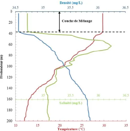
La stratification des océans se fait parce qu’il existe une différence de densité entre les eaux à la surface des océans et les eaux au fond des océans. L’action de la gravité force les couches de plus forte densité vers les fonds marins et laisse les couches de plus faible densité (dans les océans, c’est la couche de mélange) à la surface. Cette dernière se trouve donc à être continuellement brassée et mélangée par la cassure des vagues, les courants générés par le vent, les échanges de chaleur et flux causés par les différences de densité de l’eau. Puisqu’elle est continuellement mélangée, les propriétés physicochimiques y sont relativement homogènes de la surface jusqu’à sa limite sous la surface (voir figure I), appelée profondeur de la couche de

~ 3 ~

mélange (Zm; m) (voir la liste des symboles p.11-12). Selon les régions et les particularités de

celles-ci, Zm peut être aussi peu que 2 m ou aussi grande que 1000 m (e.g., de Boyer Montégut et

al., 2004; Milutinović et al., 2009). Les Zm plus faibles sont situés surtout dans les régions équatoriales en raison de l’apport important en chaleur dû à un éclairement solaire plus direct qui diminue la densité des eaux de surface. Les Zm les plus importants se retrouvent quant à elles plutôt dans les régions polaires où la faible température ainsi la salinité plus élevée due à la formation de glace augmente la densité de l’eau. Ces processus contribuent à éroder la différence

de densité entre la surface et la couche profonde et ainsi à augmenter Zm (e.g., Garrison, 2009;

Sverdrup et al., 2009).

Figure I : Densité (mg/L), température (°C) et salinité (mg/L) d’un profil vertical mesuré par une bouée Argo le 08

juin 2014 à 5.834°N et 68.451°E. Les données ont été obtenues de http://www.nodc.noaa.gov/argo/floats_data.htm. La

profondeur de la couche de mélange (Zm) est déterminée par une « cassure » de l’homogénéité des propriétés

physicochimiques de la zone à la surface, soit la température et la salinité, deux facteurs qui influencent la densité. Puisque cette couche est constamment brassée, ses propriétés vont être constantes en surface jusqu’à ce que l’action des forces qui la mélange (e.g., vent, flux thermiques) se soit estompée.

La couche de mélange est particulièrement intéressante puisqu’elle est l’environnement de croissance du phytoplancton à la surface des océans et en conséquence, directement

~ 4 ~

observable à partir de capteurs en orbite autour de la Terre. Ses propriétés sont ainsi celles auxquelles les organismes pouvant être observés par télédétection sont continuellement soumis.

Quand la stratification s’intensifie et que Zm diminue, l’apport en nutriments essentiels pour le phytoplancton se trouve à diminuer. Toutefois, l’éclairement moyen dans la couche de

mélange, appelé éclairement de croissance (Eg : µmol m-2 s-1), qui est essentielle à la

photosynthèse, va quant à lui augmenter (e.g., Behrenfeld et al., 2005). L’augmentation de Zm ainsi que la diminution de l’éclairement incident sont d’ailleurs notées comme sources importantes de la diminution de la concentration en chlorophylle ([Chl]; mg chl m-3) dans les régions polaires pendant l’hiver austral pour le Pôle Sud et pendant l’hiver boréal pour le Pôle Nord (Boyd et al., 2001; Lancelot et al., 2000; Moore et Abbott, 2002; Mitchell et al., 1991; Smith et al., 2000; Veth et al., 1997). Cette mesure de la [Chl] est généralement associée à la concentration de biomasse de phytoplancton. Puisque la grande majorité des organismes photosynthétiques (terrestres ou marins) utilisent des molécules de chlorophylle afin de capter l’énergie lumineuse, une augmentation ou une diminution de sa concentration à l’intérieur d’un

volume d’eau permet de donner un indice quant aux variations de biomasse (Morel et Prieur,

1977). Toutefois, certaines espèces de phytoplancton ont développé des mécanismes particuliers qui leur permettent d’augmenter leur efficacité photosynthétique, permettant ainsi d’effectuer de la photosynthèse alors qu’ils sont en présence de très peu d’éclairement (Horrop et al., 2014). Celles-ci ne sont toutefois pas observables par des capteurs au-dessus de la surface des océans. De plus, ces processus ne permettent pas de soutenir la production de nouveaux organismes, mais plutôt simplement aux organismes existants de survivre dans des conditions de faible éclairement (e.g., Alpine et Cloern, 1988).

Bien qu’un éclairement faible puisse être limitant, un éclairement trop important soutenu

pendant de longues périodes, comme c’est généralement le cas avec une Zm faible, peut être

néfaste et causer des dommages aux appareils photosynthétiques des organismes. Les effets

d’une diminution ou d’une augmentation de Zm peuvent donc être mitigés, mais selon Boyce et

al. (2010), la limitation en nutriments qui origine d’une plus fine couche de mélange expliquerait la diminution annuelle d’environ 1 % de la quantité de phytoplanctons qu’ils disent observer depuis la fin des années 1800. Il est toutefois bon de noter que certains doutes ont été émis quant à la validité des observations de cette étude (McQuatters-Gollop et al., 2011; Mackas, 2011;

~ 5 ~

Rykaczewski et Dunne, 2011). L’hypothèse sous-jacente reste tout de même valide. Une intensification de la stratification diminuera l’apport en nutriments provenant des fonds marins (e.g., Boyce et al., 2010).

Figure II : Éclairement de Croissance (Eg) représenté par l’ensemble de la zone jaune à l’intérieur de la zone de

mélange (Zm).

À la lumière de ces informations, il est important de se doter de moyens de mesurer la physiologie du phytoplancton en plus d’identifier les facteurs qui influencent leur physiologie dans leur environnement naturel. C’est ce que la mesure de la fluorescence promet de faire. Cette dernière a sans contredit permis de supporter le plus grand nombre de développements et de découvertes en océanographie et en biologie limnologique lors des 40 dernières années (Huot et Babin, 2010).

Quand un photon est absorbé par un organisme phytoplancton, trois procédés mutuellement distincts peuvent se produire. Le premier est que le photon sera utilisé pour la photosynthèse, le second est que l’énergie captée sera diffusée sous forme de chaleur et finalement la troisième possibilité est que le photon, après avoir perdu un peu de son énergie, sera réémis à une plus grande longueur d’onde. Ce dernier procédé est la fluorescence et c’est le seul de ces mécanismes que nous pouvons mesurer par télédétection, d’où son importance capitale pour nous aider à mieux comprendre ces organismes essentiels au maintien des conditions planétaires actuelles (Field et al., 1998).

~ 6 ~

La probabilité qu’un photon soit réémis sous forme de fluorescence est d’environ 5 %. Cette probabilité est en fait le rapport entre le nombre de photons émis et le nombre de photons absorbé, plus communément appelé rendement quantique de la fluorescence (φ : sans unité). L’éclairement incident, l’absorption du phytoplancton et le rendement quantique sont donc liés de façon intrinsèque à la fluorescence émise par la chlorophylle a. La mesure de la fluorescence est par ailleurs utilisée comme outil pour déceler la présence de phytoplancton et même, jusqu’à un certain point, d’en déterminer la concentration (Hu et al., 2005). De façon générale, pour un éclairement incident donné, la fluorescence est bien corrélée avec la concentration de

chlorophylle a ([Chl]; mg chl m-3). Ceci permet entre autres de déterminer [Chl] en normalisant

la fluorescence par l’éclairement incident dans les zones côtières où les algorithmes traditionnels (e.g., Morel et Gentili, 2009) fonctionnent moins bien en raison des grandes concentrations sédiments (e.g., Huot et al., 2005).

En normalisant davantage la fluorescence par l’éclairement incident et par l’absorption par le phytoplancton, φ peut être obtenue ce qui permet d’obtenir de l’information sur l’état physiologique des cellules. Dans un contexte d’analyse et de suivi des populations de phytoplancton, ce type d’information est extrêmement intéressante (Kiefer and Reynolds, 1992). Quelques algorithmes ont déjà été avancés pour extraire φ (e.g., Morrison, 2003; Behrenfeld et

al., 2005; Huot et al., 2005), ainsi que 𝜒𝑓𝑙𝑢𝑜 (sans unités), un indice analogue (Huot et al., 2013),

à partir de données de télédétection. Le 𝜒_{𝑓𝑙𝑢𝑜} est un indicateur obtenu à partir d’un algorithme

totalement empirique qui donne une valeur d’anomalie de la fluorescence en fonction d’un ensemble de paramètres environnementaux, soit l’éclairement incident et l’absorption par le phytoplancton (plus de détails sur cet algorithme sont donnés à la section méthodologie de

l’article). Le principe fondamental derrière le 𝜒_{𝑓𝑙𝑢𝑜} est que une fois ces deux paramètres

contrôlés, la variation (i.e., anomalie) dans la fluorescence devrait être associée au rendement quantique.

Un des principaux défis actuels avec φ ou 𝜒_{𝑓𝑙𝑢𝑜} est de parvenir à expliquer leur

distribution. Dans cette optique, 𝜒_{𝑓𝑙𝑢𝑜} peut s’avérer très utile. Bien qu’il ne donne pas la vraie

valeur physique de φ, il en imite le comportement avec des valeurs faibles lorsque φ est faible et

~ 7 ~

théoriques et semi-théoriques de φ (e.g., Morrison, 2003; Behrenfeld et al., 2005; Huot et al., 2005) puisqu’il ne fait pas de supposition quant à la valeur de certains des paramètres physiques qui entrent en ligne de compte dans le calcul de φ (Huot et al., 2013).

Le problème auquel nous sommes confrontés est qu’à ce jour, personne n’est en mesure d’expliquer les variations observées à une échelle globale du φ, bien que certaines études proposent des pistes de solutions intéressantes. Celles-ci incluent notamment la disponibilité de

certains nutriments inorganique (i.e., Fe, N, P), Eg et la température à la surface des océans (SST,

°C). Ces différentes études sont plus amplement explorées à la section discussion du chapitre 2. Généralement, les hypothèses de ces dernières sont que les facteurs environnementaux ont une influence plus ou moins importante sur la physiologie du phytoplancton ainsi que sur l’inhibition non photochimique de la fluorescence (Non Photochemical Quenching : NPQ). Ce NPQ (aussi expliqué plus amplement dans les sections suivantes) est en fait une dissipation de l’énergie lumineuse sous forme de chaleur. Il est donc logique, de tenter d’identifier les facteurs affectant

le NPQ considérant que le φ et de façon semblable le 𝜒_{𝑓𝑙𝑢𝑜} sont largement dépendants de ce type

d’inhibition. Le NPQ est à son tour influencé par l’environnement auquel le phytoplancton est acclimaté, incluant l’éclairement auquel il est soumis (Huot et al., 2005; Huot et Babin, 2010; Long et al., 1994; Pospisil 1997; Müller et Niyogi, 2001).

Avec les paramètres typiques de prise d’image, soit aux alentours de midi, quand le soleil est au zénith sous des conditions sans nuages, l’éclairement incident se trouve à être très près du

maximum journalier. Il peut avoisiner et même dépasser 2000 μmol m-2 s-1 à la surface de l’eau

pour l’ensemble du spectre de l’éclairement photosynthétiquement actif (PAR; éclairement total

entre 400 et 700 nm; μmol m-2 s-1) (NASA, 2006). Dans de telles conditions, le NPQ est la forme

d’inhibition de la fluorescence la plus importante pour les organismes qui se situent à proximité de la surface (e.g., Huot et al., 2005).

Un autre facteur pouvant influencé φ est la température de l’eau qui est mesurée de façon routinière par des capteurs tels que le MODerate resolution Imaging Spectrometer sur la plateforme Aqua (MODIS-Aqua). Ces mesures sont en fait une mesure de la température à la surface des océans (SST, °C) produite grâce à l’utilisation de bandes dans le moyen infrarouge et dans l’infrarouge lointain (Brown et al., 1999). La SST a été notée comme facteur important dans

~ 8 ~

le comportement de φ par Browning et al. (2014), qui soumettait l’hypothèse que ceci était peut-être causé par le NPQ. Il est possible que cette dépendance soit causée par une diminution de la capacité d’assimilation des électrons et d’une diminution de la capacité des processus photosynthétique à fournir des électrons telle qu’expliquée par Kiefer and Cullen (1991).

Objectifs

Afin d’aider à expliquer le comportement du rendement quantique de la fluorescence du phytoplancton, nous proposons d’évaluer les effets qu’ont différents facteurs environnementaux

sur ce dernier. Mais plutôt que de calculer directement φ nous calculons 𝜒𝑓𝑙𝑢𝑜, qui, nous

croyons, donnera une observation plus juste du réel comportement du φ que ce qu’il n’est possible d’obtenir avec les algorithmes théoriques ou semi-théoriques. Puisque nous cherchons

justement à identifier l’effet de certains facteurs sur le φ, le 𝜒𝑓𝑙𝑢𝑜 sera suffisant pour y arriver et

nos analyses ne souffriront pas du fait que nous ne calculons pas la valeur physique réelle de φ.

Hypothèses

Nous émettons l’hypothèse que le 𝜒𝑓𝑙𝑢𝑜 devrait être influencé par Eg en diminuant quand

Eg augmente et en augmentant quand Eg diminue, en raison de la relation existante entre le NPQ

et Eg, notamment en raison des mécanismes de photoprotection et du photodomage. Autrement

dit, on s’attend à observer une plus grande inhibition de la fluorescence lorsqu’Eg est plus élevé

en raison d’une acclimatation accrue à de forts éclairements.

Sites d’étude

Pour cette étude, aucun site particulier n’est ciblé. C’est plutôt l’ensemble des océans pour lesquels des données sont disponibles de mai à septembre 2006 inclusivement qui sera

considéré. Toutefois, les régions ou la [Chl] est inférieur à 0.1 mg chl m-3 sont à éviter puisque la

fluorescence ne peut être mesurée correctement dans ces conditions. À ces niveaux de [Chl], les algorithmes qui récupèrent le rayonnement provenant de la fluorescence ne sont pas en mesure de distinguer ce dernier du rayonnement de fond (Franz et al., 2006; Meister and Franz, 2011; Huot et al., 2013). Ceci peut donner des aberrations physiques comme un rayonnement de

~ 9 ~

fluorescence négatif. Ces zones de basse chlorophylle couvrent environ 30 % de la surface des océans, mais représentent moins de 10 % du total de la biomasse (Antoine et al., 2005).

Une attention particulière sera portée à l’océan Atlantique Nord, l’océan Pacifique Nord

et à l’océan Austral en raison des différences qu’ils affichent en terme de 𝜒𝑓𝑙𝑢𝑜 lors des mois de

juin, juillet et août (Huot et al., 2013). Le 𝜒𝑓𝑙𝑢𝑜 est généralement élevé en Atlantique Nord, alors

qu’il peut varier de façon importante dans le Pacifique Nord et dans l’océan Austral. Ces

différences sont intéressantes pour évaluer la relation entre 𝜒𝑓𝑙𝑢𝑜 et certains paramètres

~ 10 ~

Chapitre 2: Article

--Soumis à Remote sensing of Environment le 9 septembre 2015--

The influence of growth irradiance and of the sea surface temperature on the quantum yield of Sun-induced fluorescence

Marc-André Faucher and Yannick Huot

Abstract

The current generation of Earth-orbiting sensors allows us to measure Sun-induced chlorophyll fluorescence. Coupled with phytoplankton absorption and incident irradiance, it is possible to derive the apparent quantum yield of chlorophyll fluorescence. This information could be very helpful as the apparent quantum yield of chlorophyll fluorescence is influenced by algal photophysiology. Here we evaluate the influence of the growth irradiance and of the sea surface temperature on the apparent quantum yield of chlorophyll fluorescence. Results show that with increasing growth irradiance, the apparent quantum yield of chlorophyll fluorescence decreases, pointing to an increase in non-photochemical quenching due to photoacclimation/photoadaptation by phytoplankton in high light environments. The sea surface temperature below 6°C was shown to have a significant impact on the apparent quantum yield of chlorophyll fluorescence. Below this temperature, a group of pixels was identified for which the apparent quantum yield of chlorophyll fluorescence was essentially constant at low values. This could potentially point to a wider ecosystemic/community related phenomenon. Simulations with a three-dimensional lookup table (i.e., growth irradiance, sea surface temperature and chlorophyll concentration) demonstrate the impact of these parameters on the global distribution of the apparent quantum yield of chlorophyll fluorescence. The model successfully reproduced

~ 11 ~

some zones of low and high yield. Departures from the predicted values are likely pointing to physiological processes that are independent of temperature and growth irradiance.

Keywords

Quantum yield, Sun-induced chlorophyll a fluorescence, growth irradiance, sea surface temperature, global analysis, MODIS.

Notation table

Symbol Definition Unit

aCDOM CDOM absorption coefficient m-1

a𝜙 Phytoplankton absorption coefficient m-1

𝑎_𝜙∗ Chlorophyll specific absorption coefficient m2 (mg chl)-1

[Chl] Chlorophyll a concentration mg chl m-3

CDOM Colored Dissolved Organic Matter

Eg Growth irradiance μmol photons m-2 s-1

Ed Downwelling irradiance μmol photons m-2 s-1

nm-1

Ed(0+, PAR) Downwelling PAR irradiance directly above the water surface μmol photons m-2 s-1

Ēd(0-, PAR) Daily averaged incident downwelling PAR irradiance directly

below the water surface

mol photons m-2 day-1

ET Light saturation parameter of energy dependant quenching μmol photons m-2 s-1

Kd Diffuse attenuation coefficient of downwelling irradiance m-1

Kdbio Diffuse attenuation coefficient of downwelling irradiance

associated with all the biogenic components

m-1

Kdw Diffuse attenuation coefficient of downwelling irradiance for

pure water m

-1

Lf Fluorescence radiance mW cm-2 sr-1 μm-1

nLw Normalized water leaving radiance mW cm-2 sr-1 μm-1

nFLH Fluorescence Line Height from normalized water leaving

radiance

mW cm-2 sr-1 μm-1

PAR Photosynthetically Available Radiance μmol photons m-2 s-1

~ 12 ~

Rrs Remote Sensing Reflectance sr-1

SST Sea Surface Temperature °C

Zm Mixed layer depth m

λ Wavelength nm

𝜑 Quantum yield of fluorescence unitless

𝜑_𝑚𝑖𝑛 Minimum quantum yield of fluorescence unitless

𝜑_𝑚𝑎𝑥 Maximum quantum yield of fluorescence unitless

𝜑_𝑓𝑎𝑝𝑝 Apparent quantum yield of fluorescence unitless

𝜒_{𝑓𝑙𝑢𝑜} Alternate measure of 𝜑_𝑓𝑎𝑝𝑝 (Huot et al. 2013) unitless

1. Introduction

The measurement of Sun-induced chlorophyll fluorescence, coupled with phytoplankton absorption and incident irradiance, allows the measurement of the apparent quantum yield of

chlorophyll fluorescence (𝜑_𝑓𝑎𝑝𝑝, unitless), which is defined as the ratio of photons reemitted as

fluorescence to the photons absorbed by all phytoplankton pigments (e.g., Huot et al., 2005). This quantum yield contains information about phytoplankton physiology (Cleveland and Perry, 1987; Babin et. al., 1996; Laney et al. 2005). The recent generation of Earth-orbiting sensors, such as the MODerate resolution Imaging Spectrometer on the Aqua platform (MODIS-Aqua) or the MEdium Resolution Imaging Spectrometer (MERIS) on the Envisat platform, can measure

𝜑_𝑓𝑎𝑝𝑝 on global scales, which could potentially allow the monitoring of phytoplankton

physiology on large scales. While it has been over 35 years since Morel and Prieur (1977) and Neville and Gower (1977) proposed that chlorophyll a fluorescence could be measured in the ocean’s upwelling light field and over 16 years since we can observe it from space after MODIS TERRA’s launch, progress has been slow to understand the most important sources of variability in the global distribution of 𝜑_𝑓𝑎𝑝𝑝.

~ 13 ~

When a chlorophyll molecule within a phytoplankton cell absorbs light (or is excited by energy transfer from another pigment), the energy of the absorbed photons can be transformed in three mutually exclusive paths: photosynthesis, dissipation as heat, or fluorescence (centered at ca. 685 nm). Of these processes, only fluorescence can be measured remotely (Neville and Gower, 1977; Morel and Prieur, 1977; Gordon 1979). The chlorophyll fluorescence radiance that

originates from a small volume of water (Lf, mW m-2 μm-1 sr-1) depends on three variables: (1)

the phytoplankton absorption coefficient (aϕ, m-1); (2) the incident downwelling irradiance (Ed,

μmol m-2 s-1) in the photosynthetically available radiation (PAR, spectral range of solar radiation

from 400 to 700 nm) portion of the spectrum [Ed(PAR)], and; (3) 𝜑_𝑓𝑎𝑝𝑝. While accounting for optical and spectral effects within the water column requires more complex models to obtain

𝜑_𝑓𝑎𝑝𝑝 (e.g., Maritorena et al., 2000; Huot et al., 2005, 2013; Behrenfeld et al., 2009), a simplified

model of fluorescence emission can be written as follows:

𝐿_𝑓 ∝ 𝑎_𝜙 𝐸_𝑑(PAR) 𝜑_𝑓𝑎𝑝𝑝 (1)

From eq. 1, it is clear that dividing Lf by aϕ and Ed(PAR) is necessary to obtain 𝜑_𝑓𝑎𝑝𝑝, which contains the physiological information that is sought (Falkowski and Kiefer, 1985; Babin et. al., 1996; Cullen et al., 1997; Ostrowska et al., 1997; Maritorena et al., 2000; Morrison, 2003; Westberry et al., 2003; Laney et al., 2005; Huot et al., 2007; Schallenberg et al., 2008). Given

𝜑_𝑓𝑎𝑝𝑝, however, deriving physiological information is not a straightforward process as there are

many potential influences.

Within the cell at least four genetically and physiologically controlled processes act as

~ 14 ~

associated with photosystem II (PSII) over the total absorbed light by all pigments (see Huot et al., 2005, Appendix 2); (2) photochemical quenching (PQ); (3) non-photochemical quenching (NPQ) (Long et al., 1994; Pospisil, 1997; Müller et al., 2001); and (4) the intrinsic quantum yield of chlorophyll within the PSII antenna. The fluorescence around 685 nm almost exclusively originates from PSII, hence the importance of considering the fraction of light absorbed by it. Furthermore, only photosynthetic pigments within PSII will transfer their excitation to

chlorophylls within the antenna and allow fluorescence to occur. PQ is a decrease of 𝜑_𝑓𝑎𝑝𝑝

caused by an increase in the quantum yield of photochemistry at low irradiance. NPQ leads to a decrease of 𝜑_𝑓𝑎𝑝𝑝 and is present predominantly at high irradiance. It is caused by an increased dissipation of absorbed energy as heat (Krause et Weis, 1991). NPQ can originate from damage or inactivation of reaction centers or photoprotection processes (Krause and Jahns, 2004). These mechanisms allow the excitation energy transfer to PSII to be matched to the photochemical utilization in order to protect them from oxidative damage (Horton et al., 1994). All of these processes are in turn influenced by the growth conditions and the species present (Loftus and Seliger, 1975; Vincent, 1979, 1980; Cullen and Ranger, 1979; Falkowski and Kiefer, 1985).

Since sensors on polar-orbiting satellites acquire ocean color data around mid-day under cloud-free conditions, and observe only the top 2 to 3 m of the ocean (e.g., Babin et al., 1996; Mobley, 2004; Huot and Babin, 2010), the irradiance is about the highest experienced by phytoplankton in these waters. They are thus in a light-regulated state in which NPQ is the prime quenching mechanism, likely making it, together with the fraction of absorbed energy by

photosynthetic pigments in PSII, the most important proximate controls on 𝜑_𝑓𝑎𝑝𝑝 (Huot et al.,

~ 15 ~ 1.1 Assessing the global variations of 𝝋_𝒇𝒂𝒑𝒑

While the proximate controls described above have been known for some time, their modulation by environmental variables, either directly or through shifts in species composition, remains to be understood. Several studies have proposed different potential sources of variability

for 𝜑_𝑓𝑎𝑝𝑝. The incident (Behrenfeld et al., 2009) and growth irradiance (Morrison and Goodwin,

2010; O’Malley et al., 2014), nutrient stress (Letelier et al., 1997; Schallenberg et al., 2008; Behrenfeld et al., 2009; Westberry et al., 2013), and water temperature (Browning et al., 2014) have all been proposed as potential sources of variability, while species composition is observed to have a strong impact on fluorescence yields and measurements (Loftus and Seliger, 1975, Jolliff et al., 2012; Suggett et al., 2009).

The growth irradiance (Eg, μmol m-2 s-1) is defined here as the average irradiance between

the surface and the bottom of the mixed layer (Zm, m). Due to the limited depth observed by

sensors that measure the radiance near 680 nm, most of Lf will originate from phytoplankton

within this layer. As a response to Eg, the phytoplankton community will either: 1)

photoacclimate (changes in the molecular constituents of the cells occurring on the order of a day); or 2) its composition will be modified (changes in their genetic makeup occurring on the order of several days to weeks) as species more photoadapted to the new conditions outcompete the species previously present. Both of these processes, as well as mixing events in stratified water that can bring low light adapted/acclimated cells to the surface, will alter some of the four proximate controls of 𝜑_𝑓𝑎𝑝𝑝 measured in surface waters. In addition to altering 𝜑_𝑓𝑎𝑝𝑝, these

changes will also modify the overall aϕ through changes in the pigment composition and package

~ 16 ~

spectral change in 𝑎_𝜙∗ _{due to pigment packaging or pigment composition that does not follow the}

mean oceanic trend between 𝑎_𝜙∗ _{and remote sensing reflectance band ratios will lead to biases in}

the estimate of aϕ (e.g., Uitz et al. 2006, 2008; Morel et Gentili, 2009) and erroneous estimates of

𝜑_𝑓𝑎𝑝𝑝 (which, without in situ validation, could be interpreted as real variations in 𝜑_𝑓𝑎𝑝𝑝). The cumulative effect of the changes due to growth irradiance was suggested as playing a key role in

explaining the variability in 𝜑_𝑓𝑎𝑝𝑝on Georges Bank (Morrison and Goodwin, 2010) and in the

Philippines Sea (O’Malley et al., 2014). In both cases, observations show an increase in the quantum yield of fluorescence under deep-mixing conditions. Different modeling approaches in both studies have assigned this effect to reduced non-photochemical quenching at high growth irradiance.

Nutrient stress in phytoplankton has long been studied for its impact on these organisms (e.g., Geider et al., 1993; Kolber et al., 1994; Coale et al., 1996 and 1998; Johnson et al., 2001; Parkhill et al., 2001; Behrenfeld et al., 2009). In large swaths of the ocean, iron (Fe) limits phytoplankton growth and alters its community structure and abundance (e.g., Boyd et al., 2007).

Comparison of an ecosystem model with remote measurements of 𝜑_𝑓𝑎𝑝𝑝 in the global ocean has

shown that regions where Fe limitation is present tend towards higher 𝜑_𝑓𝑎𝑝𝑝 (Behrenfeld et al.,

2009). Shipboard experiments in the Southern Ocean showed that Fe limitation was indeed an

important factor controlling 𝜑_𝑓𝑎𝑝𝑝 (Browning et al., 2014), while a study of previous in situ Fe

enrichment experiments has shown that alleviation of Fe limitation leads to a reduced 𝜑_𝑓𝑎𝑝𝑝

(Westberry et al., 2013). Together, these studies suggest that once the impact of incident irradiance is appropriately corrected, Fe limitation is a key environmental control of the large-scale variations in 𝜑_𝑓𝑎𝑝𝑝. Based on several studies that show an increase of the PSII:PSI ratio

~ 17 ~

with Fe limitation (Sandmann, 1985; Vassiliev et al. 1995, Ivanov et al., 2000; Strzepek and Harrison, 2004), it was hypothesized (Behrenfeld et al., 2009) that such changes were

responsible for the higher 𝜑_𝑓𝑎𝑝𝑝 observed under these conditions. However, field experiments in

the North Atlantic have shown that the PSII:PSI ratio appears to be independent of Fe stress at the community level (Macey et al. 2014). In addition, laboratory experiments (Burnap et al., 1993; Schrader et al., 2011, Ryan-Keogh et al., 2012) have shown that under high Fe stress

Synechococcus sp. and Synechocystis sp. synthesize chlorophyll-binding protein complexes that

are dissociated from the reaction centers and thereby have high fluorescence quantum yields, thus offering an alternative explanation for the high yields observed under Fe stress.

The impact of water temperature on 𝜑_𝑓𝑎𝑝𝑝 , under in situ conditions where

photoacclimation and photoadaptation has taken place, is largely unknown. Recently, Browning

et al. (2014) found a strong correlation between SST and 𝜑_𝑓𝑎𝑝𝑝 due to enhanced NPQ at low

temperatures. Their study did not elucidate the cause of this temperature effect but the authors suggested that the temperature might be reflecting the lower growth irradiance encountered in the deeply mixed layer of the Southern Ocean, instead of having a direct causal link to increased NPQ. Different water temperatures will also lead to different species compositions (e.g., Claustre et al., 2005; Litchman et al., 2007; van de Poll et al., 2013).

Species composition will undoubtedly have some impact on 𝜑_𝑓𝑎𝑝𝑝. Different species can

grow, acclimate and photoadapt to a given growth environment. Additionally, species-specific differences such as pigment composition, photosynthetic antenna structure, pigment packaging or growth rate (Falkowski et al., 1985) were all previously explored as important factors

~ 18 ~

Given the limited range of measured 𝜑_𝑓𝑎𝑝𝑝 in the surface ocean, estimating it accurately

from remote sensing is far from trivial since even small biases can overwhelm the natural

variability. Several algorithms have been proposed to obtain 𝜑_𝑓𝑎𝑝𝑝 based on estimates of a𝜙, Lf,

and incident irradiance as well as empirical relationships between [Chl] or the diffuse attenuation

coefficient for downwelling irradiance (Kd, m-1) and the optical properties of water (e.g., Babin et

al., 1996; Morrison 2003; Huot et al., 2005; Behrenfeld et al., 2009). Recently, Huot et al. (2013)

proposed a new method to obtain a proxy of 𝜑_𝑓𝑎𝑝𝑝 using a parameter called 𝜒𝑓𝑙𝑢𝑜. This new

empirical model departs from the previous and more complex semi-empirical models listed above in important ways. The advantage of Huot et al.’s (2013) model over the semi-empirical

ones lies in the fact that it does not use empirical relationships between [Chl] or Kd and various

algal or oceanic properties and, therefore, it reduces potential biases. It accounts implicitly for

the complex spectral effects. Finally, it accounts for the combined effects of aϕ, Colored

Dissolved Organic Matter absorption (aCDOM, m-1) and Ed(PAR).

This study examines the potential sources of variations in 𝜒_{𝑓𝑙𝑢𝑜} at the global scale by

~ 19 ~

2. Methods

2.1 Data sources

Data from two sources were used during this study. The first is from the MODIS-Aqua sensor and the second is the HYbrid Coordinate Ocean Model (HYCOM). The MODIS-Aqua daily level-3 Standard Mapped Image data products (see Table 1 for the complete list of data products used in this study) at a resolution of 9 km for the months of May to September 2006

were downloaded from the NASA ocean color website (http://oceancolor.gsfc.nasa.gov/). In both

cases, values were obtained for the whole ocean but the fluorescence and ocean color products were only available above 67°S at this time of the year due to the low irradiance at higher southern latitudes.

Table 1: Data products used in the present study. All the data products are from MODIS-Aqua measurements/algorithms except for the mixed layer depth generated by the HYCOM model.

Data products used (symbol, units) [derived variable]

Chlorophyll concentration ([Chl], mg chl m-3) [Eg and 𝝌𝒇𝒍𝒖𝒐]

Daily average photosynthetically available radiation (𝐸̅_𝑑(PAR), mol m-2 day-1) [Eg]

Mixed layer depth (Zm: m) [Eg]

Remote sensing reflectance (Rrs(412), sr-1) at 412, 443, 488 and 547 nm [𝝌_{𝒇𝒍𝒖𝒐}]

Fluorescence line height (nFLH, mW m-2 sr-1 μm-1) [𝝌𝒇𝒍𝒖𝒐]

Instantaneous photosynthetically available radiation (𝐸_𝑑(0+_{, PAR), μmol m}-2 _s-1_{) [𝝌} 𝒇𝒍𝒖𝒐] Colored Dissolved Detrital Matter Index (CDOM Index, Morel and Gentili [2009]) Daytime sea surface temperature (SST: °C)

~ 20 ~

The time period was selected because the calibration for band 14 (678 nm) was more or less constant throughout those months (Meister et al., 2012). This is crucial since the 678 nm

band is used in the algorithm for the Fluorescence Line Height product (nFLH, W m-2 sr-1 μm-1)

obtained from the normalized water-leaving radiance. In theory, the nFLH represents the upwelling radiant energy originating only from fluorescence. Physically, the fluorescence emission cannot be less than zero and negative values from the nFLH product are generally considered incorrect and set to zero during the standard level-3 data processing distributed by NASA (see Behrenfeld et al., 2009). However, Huot et al. (2013) suggested that the nFLH product’s negative values result from sensor noise and are part of the normal distribution of points in oligotrophic waters and should thus be kept. The nFLH product used in this study was therefore reprocessed by Bryan Franz (NASA ocean color group) to level-3 to include the negative values.

The HYCOM’s global assimilative experiment (GLBa0.08/epx_60.5) daily values of Zm

were downloaded from HYCOM’s FTP data server

(ftp://ftp.hycom.org/datasets/GLBa0.08/expt_60.5/) for the same time period as the MODIS data. HYCOM’s GLBa0.08/expt_60.5 uses HYCOM’s forecast model as a first estimate and further uses the Navy Coupled Ocean Data Assimilation (NCODA) system (Cummings, 2005) to reduce biases using satellite and in situ measurements. These results are available daily for the global ocean on a 1/12° grid (~9 km at the equator).

2.2 Growth irradiance algorithm

We use photosynthetically usable radiation (PUR; Morel, 1978) as a measure of

~ 21 ~

of Eg than PAR as it weights spectral irradiance according to phytoplankton absorption.

Therefore, we define our estimate of Eg as the Ed(PUR) average between the surface and Zm,

𝐸_𝑔 = _𝑍1

𝑚∫ 𝐸𝑑(𝑍, PUR)

𝑍𝑚

0 𝑑𝑍, (2)

where Z is the depth (m) and Ed(Z, PUR) is a slightly modified version of Morel’s (1978)

description, 𝐸𝑑(Z, PUR) = ∫ 𝑎_𝜙∗(𝑍,𝜆) max [𝑎_𝜙∗(𝑍,𝜆)] 𝜆=700 𝜆=400 𝐸𝑑(Z, 𝜆) 𝑑𝜆. (3)

where we use the chlorophyll specific absorption coefficient (𝑎_𝜙∗ _{= a}

𝜙 / [Chl]) instead of Morel’s

a𝜙; max[𝑎_𝜙∗ (Z, λ)] represents the maximum value of the 𝑎_𝜙∗ (Z, λ) spectrum and λ is the

wavelength (nm). Since 𝑎_𝜙∗ and a𝜙 have the same shape for a given absorption spectrum, and the

computation uses the spectrum scaled to its maximum, the resulting Ed(Z, PUR) are exactly the

same. By switching a𝜙 by 𝑎_𝜙∗, the spectral shape required in eq. 2 can now be calculated at depth

Z following the model of Uitz et al. (2008) for a given surface chlorophyll concentration. The

downwelling irradiance at depth Z [Ed(Z, λ) μmol m-2 s-1] is computed using:

𝐸_𝑑(𝑍, 𝜆) = 𝐸_𝑑(0−_{, 𝜆) 𝑒}−𝐾𝑑(𝜆) 𝑍 (4)

where [Ed(0–, λ), μmol photons m-2 s-1] is the planar downwelling irradiance just below the

sea-surface.

The spectral shapes for Ed(0–, λ) and Kd(λ) are not available as standard MODIS-Aqua

products and need to be estimated from available remote sensing data. The Ed(0–, λ) spectrum is

~ 22 ~

spectrum by the daily PAR irradiance provided as part of the MODIS-Aqua data products (see Table 1). This method first uses the Gregg and Carder (1990) model to generate a representative

solar spectrum for the instantaneous PAR irradiance [Ed(0–, λ)GC90;μmol m-2 s-1]. We generated

our solar spectrum for the subtropics during the month of June under midday clear sky

conditions. The daily average PAR irradiance [Ēd(PAR), mol m-2 day-1] estimated at just below

the surface (i.e. at 0-) is essentially a scaling parameter for the spectrum generated by the Gregg

and Carder (1990) model. To do this, Ed(0–, λ)GC90 is normalized to the model’s daily average of

PAR irradiance [Ēd(0–, PAR)GC90, mol m-2 day-1] for the same spectrum. This ratio is then

multiplied by Ēd(PAR):

𝐸_𝑑(0−_{, 𝜆) = 𝐸̅}

𝑑(PAR)[ 𝐸𝑑(0−, 𝜆)GC90 /𝐸̅𝑑(0−, PAR)GC90] (5)

The Behrenfeld et al. (2009) approach allows an estimate of the spectral downwelling irradiance, Ed(0–, λ), for each pixel based on the Ēd(PAR) NASA data product. This method yields results that are similar to more complex radiative transfer models under significant variations of illumination conditions [within 1-6% depending on the wavelength (Westberry et al., 2008)]. Since the shape of the incident spectrum does not change, the differences between PAR and PUR in our method occur within the water column where it accounts for varying absorption and diffuse attenuation spectra.

The Kd(λ) value is estimated using an algorithm from Morel et al., (2007): Pigment

algorithms: Second approach. This model only requires [Chl] as an input (the MODIS-Aqua

chlorophyll concentration product) to determine the Kd(λ) associated with algal cells and

covarying material denoted Kdbio(λ) (Morel and Maritorenna, 2001). The Kdbio(λ) value is then added to the diffuse attenuation coefficient of pure water [Kdw(λ), m-1] to obtain Kd(λ).

~ 23 ~

With the Ed(0–, λ), Kd(λ) and 𝑎𝜙∗ spectra, Ed(Z, PUR) can be calculated at any depth using

equation 4. We do so every meter between the surface and Zm and vertically integrate the

resulting Ed(Z, PUR) using a trapezoidal integration. The result is then divided by Zm to obtain Eg

(equation 2).

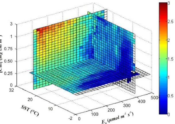
2.3 𝝌_{𝒇𝒍𝒖𝒐} algorithm

As mentioned earlier, 𝜑_𝑓𝑎𝑝𝑝 is not directly calculated. Instead, the Huot et al. (2013) algorithm is used to derive 𝜒_{𝑓𝑙𝑢𝑜}. This algorithm is based on the use of a three dimensional lookup table (LUT) which accounts for most of the optical effects, other than the quantum yield, that can be measured by satellite sensors and affect the fluorescence emission. The three inputs to this LUT are: (1) the ratio of the remote sensing reflectance (𝑅_𝑟𝑠, sr-1) at 412 and 443 nm

(443412𝑅𝑟𝑠, unitless); (2) the Maximum Band Ratio (MBR, unitless), which is the maximum Rrs at

443 or 489 nm divided by the 𝑅𝑟𝑠 at 547 nm; and (3) the Ed(0+, PAR) from the MODIS iPAR

algorithm. The ₄₄₃412𝑅_{𝑟𝑠 and MBR are used to properly account for a}

CDOM and aϕ while Ed(0+, PAR) accounts for the effects of the incident irradiance on the fluorescence emission. The

LUT’s output is the median value of nFLH (nFLHLUT, W m-2 sr-1 μm-1) for the whole ocean and

all seasons for a given combination of input values. The nFLHLUT can be thought of as a typical

fluorescence emission from phytoplankton for a given a𝜙, aCDOM and Ed(0+, PAR). By dividing a

pixel’s nFLH value by its corresponding nFLHLUT, we obtain the ratio of a pixel’s fluorescence

emission to that of the median for the whole ocean under the same conditions, thereby providing

an anomaly. This is the 𝜒_{𝑓𝑙𝑢𝑜} parameter. The main assumption underlying this algorithm is that

most of the variability in nFLH, once the inputs of the LUT have been accounted for, is due to the quantum yield of fluorescence. This assumption is the same assumption made by all other

~ 24 ~

quantum yield algorithms (Huot et al., 2013). Another assumption is that the average quantum yield is the same for all chlorophyll concentrations. If this was not the case, 𝜒_{𝑓𝑙𝑢𝑜} would still provide the ratio of the quantum yield for a given pixel divided by the average of all pixels with

the same chlorophyll concentration (MBR), aCDOM (as it affects the 443412𝑅𝑟𝑠 for a given MBR) and

Ed(0+, PAR) but would not reproduce any existing average trend in 𝜑_𝑓𝑎𝑝𝑝 with chlorophyll concentration.

For all the variables above, we randomly extracted more than 37 000 000 entries (pixels) over the whole ocean and stored them in a database. Each database entry consists of a pixel for

which the 𝜒_{𝑓𝑙𝑢𝑜} and Eg values have been calculated. The database also contains the values for the

different MODIS-Aqua data products, as well as HYCOM’s Zm (see Table 1).

3. Results

3.1 Overview of data

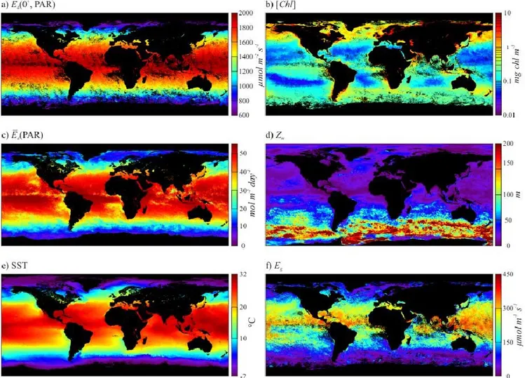
Since the data used was acquired from May through September; the equatorial and northern oceans were subject to higher daily irradiance for most of this period. However, for the month of September (Fig. 1c), which includes an equinox, both hemisphere received similar

Ēd(PAR). Note that Ēd(PAR) represents the daily integrated PAR irradiance at the surface and

includes the effect of clouds, while Ed(0+, PAR) (Fig. 1a) is the irradiance at the time of the

satellite overpass and is only computed for cloudless conditions. The variability in Ēd(PAR) is

reflected in Eg (Fig. 1f). In addition, the depth of the mixed layer (which was deeper south of

~ 25 ~

Fig. 1b) also have a significant influence over Eg and can be observed by comparing it’s patterns

to those of Zm and Ēd(PAR).

Figure 1: Global distribution for the month of September 2006 of: a) Ed(0+, PAR) ; b) [Chl]; c) 𝑬̅𝒅(𝐏𝐀𝐑); d) Zm; e)

SST, and; f) Eg.

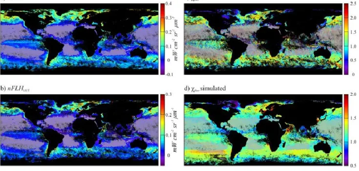
The look up table output, nFLHLUT (Fig. 2b) captures much of the large scale variability

in nFLH (Fig. 2a), which arises largely from changes in [Chl] (see Fig. 1b). The 𝜒𝑓𝑙𝑢𝑜, the result

of dividing nFLH by nFLHLUT values were slightly higher than anticipated (Fig. 2c) with an

average of ~1.2 for the complete dataset. The nature of 𝜒𝑓𝑙𝑢𝑜 should yield an average of ~1

(Huot et al., 2013). However, Huot et al., (2013) built their LUT with data from 2007. Additionally, the data used to build the LUT was corrected to account for the average presence of clouds to obtain a spatially representative dataset. We used data from 2006 that were not

~ 26 ~

corrected for the average presence of clouds. Therefore our data represents the dataset as it is observed by MODIS and some of the differences could be caused by the different spatial selection of pixels. Nevertheless, the slightly higher average is, at least partly, caused by a drift in the sensor sensitivity between the two years that was not completely accounted for in the 678 nm band calibration table, with higher values in 2006 (Meister et al., 2012).

Figure 2: Global distribution for the month of September 2006 of: a) nFLH; b) nFLHLUT; c) 𝝌𝒇𝒍𝒖𝒐; d) 𝝌𝒇𝒍𝒖𝒐

simulated, and; e) Ratio between observed and simulated 𝝌𝒇𝒍𝒖𝒐. The areas with [Chl] < 0.1 mg chl m-3 were greyed

out in the figures as MODIS-Aqua’s nFLH product is likely heavily impacted by residual sensor noise at these lower concentrations.

Variations in 𝜒_{𝑓𝑙𝑢𝑜}, for the randomly sampled subset of the global ocean, were analyzed

~ 27 ~

from the MODIS-Aqua Sea Surface Temperature (11 μm algorithm daytime) product, Eg, as well

as Ēd(PAR) and Zm, which are both used in the calculation of Eg.

Both [Chl] and Ed(0+, PAR) are also included in Figure 3 which shows that both have little effect on 𝜒_{𝑓𝑙𝑢𝑜} as they are accounted for in Huot et al.’s (2013) algorithm. Nonetheles, there is an increase in the variability in 𝜒_{𝑓𝑙𝑢𝑜} at lower [Chl]. While developing the 𝜒_{𝑓𝑙𝑢𝑜}

algorithm, Huot et al. (2013) found a similar effect in the nFLH product due to Lf approaching

and eventually falling below the detection limits of the sensor as [Chl] decreases. This increase

in variability is also present at high Ed(0+, PAR) (Fig. 3f) which can be due to increased NPQ or

because Ed(0+, PAR) tends to be higher in and around the tropics where [Chl] is low (Fig 1a and

b).

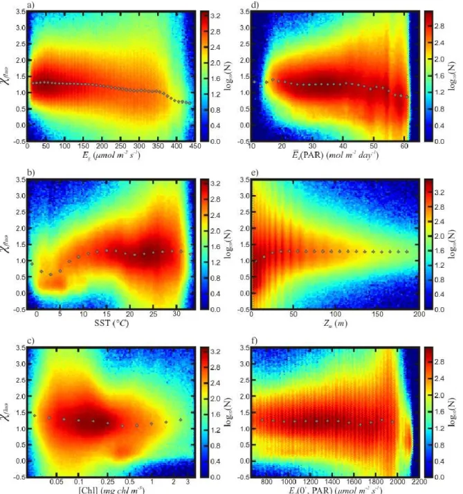
Despite significant variability, global 𝜒𝑓𝑙𝑢𝑜 values tend to decrease slightly with

increasing Eg (Fig. 3a). The median values range from ~1.3 at low Eg to ~0.6 at higher Eg. The

most significant change occurs around 350 μmol m-2 s-1, where 𝜒𝑓𝑙𝑢𝑜 drops rapidly until it

stabilizes at ~400 μmol m-2 s-1. In a similar manner, 𝜒_{𝑓𝑙𝑢𝑜} declines either when Ēd(PAR) is high

(i.e., Ēd(PAR) > ~50 mol m-2 day-1; Fig. 3d) or when Zm is shallow (i.e., 𝑍𝑚 < ~20 m; Fig. 3e), both leading to higher Eg. The remaining range for both Ēd(PAR) and Zm seems to have little effect.

~ 28 ~

Figure 3: 𝝌𝒇𝒍𝒖𝒐 as a function of: a) Eg,; b) SST; c) [Chl] presented on a logarithmic scale; d) 𝑬̅𝒅(𝐏𝐀𝐑); e) Zm , and;

f) Ed(0+, PAR) for the months of May to September 2006. The colors represent the logarithm to the base 10 of the

number of points sampled. The grey points represent the median 𝝌𝒇𝒍𝒖𝒐value for a given range of the X axis.

A rapid increase in 𝜒𝑓𝑙𝑢𝑜 was observed when SST went from 6°C to 10°C (Fig. 3b), after

which 𝜒_{𝑓𝑙𝑢𝑜} remains mostly constant at ~1.3. Below 6°C, the median is around 0.6. At these

lower temperatures, a group of points centered at 𝜒_{𝑓𝑙𝑢𝑜} values of 0.3 can be identified as

~ 29 ~

group. It was found that these points were, for the most part, located in the Arctic Ocean and at

higher latitudes. These results indicate that SST, or other processes mainly present in the colder waters of the Arctic Ocean and higher latitudes, are important determinants of global variations in 𝜒_{𝑓𝑙𝑢𝑜}.

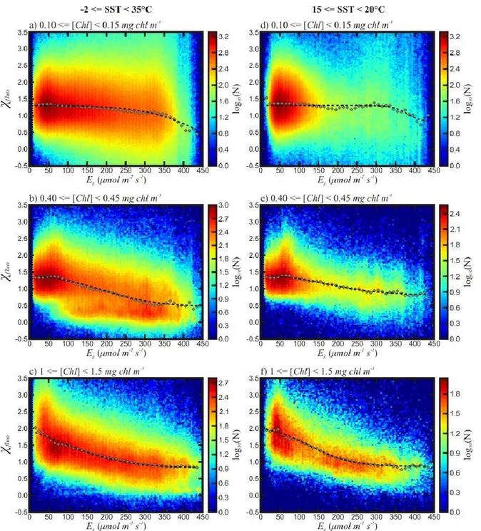
Figure 4: The 𝝌𝒇𝒍𝒖𝒐 as a function of Eg for different intervals of [Chl] (lines) for the months of May to September

~ 30 ~

the “cold waters group” (see text). The colors represent the logarithm to the base 10 of the number of points. The grey points representation of the median 𝝌𝒇𝒍𝒖𝒐 values at 10 μmol m-2 s-1 intervals in Eg. The dashed line is the

negated translated sigmoidal function that best fits the median values. This function is 𝒇(𝒙) = 𝒚𝒎𝒂𝒙−

[𝒚𝒓𝒂𝒏𝒈𝒆⁄(𝟏 + 𝒆−𝜶(𝒙−𝒄))]; where 𝒚𝒎𝒂𝒙 is the maximum on the y axis, 𝒚𝒓𝒂𝒏𝒈𝒆 is the extent on the y axis (i.e. 𝒚𝒎𝒊𝒏=

𝒚𝒎𝒂𝒙− 𝒚𝒓𝒂𝒏𝒈𝒆), 𝜶 is the slope between 𝒚𝒎𝒊𝒏 and 𝒚𝒎𝒂𝒙 and 𝒄 is the x coordinate of the inflection point.

The cold waters group identified from the SST graph is also present in the [Chl] graphs

(Fig. 3c) and occurs mainly between 0.3 and 0.6 mg chl m-3. To examine more closely the

interaction between these different variables, we proceeded to create a series of subgroups based on their [Chl].

The plots of 𝜒_{𝑓𝑙𝑢𝑜} vs. Eg for different [Chl] intervals show important differences in the

dispersion of 𝜒𝑓𝑙𝑢𝑜 as well as the response of 𝜒𝑓𝑙𝑢𝑜 to changing Eg (Fig. 4), where 3 of the 25

[Chl] groups are shown as examples). The highest variability about the mean is observed in lower [Chl] [i.e., [Chl] < 0.2 mg chl m-3], where the standard deviation () is ~0.9. The variability then gradually decreases until the dispersion around the mean trend is constant for all

[Chl] groups. This occurs at ~0.3 mg chl m-3, after which the standard deviation is close to 0.5.

The relationship between 𝜒𝑓𝑙𝑢𝑜 and Eg transitions from one shape to another smoothly as

[Chl] increases (Fig. 5a). The trend for [Chl] < 0.2 mg chl m-3 are similar to the global trend seen

in Fig. 3a, where there is a plateau in 𝜒_{𝑓𝑙𝑢𝑜} values at low Eg that extends to ~350 μmol m-2 s-1,

after which there is a decrease in 𝜒𝑓𝑙𝑢𝑜 until Eg approaches 400 μmol m-2 s-1, where it stabilizes.

The resemblance with the whole dataset is not surprising as these waters encompass ~30% of the global ocean area (Antoine et al., 2005). A transition away from this shape starts to occur

between [Chl] values of 0.3 and 0.7 mg chl m-3. This interval was previously identified in Figure

3c as being influenced by the cold waters group. This transition is, as a result, strongly

~ 31 ~

with regard to Eg. We define a second group, hereafter referred to as the warm waters group (the

whole dataset minus the cold waters group) that showed a decrease in 𝜒_{𝑓𝑙𝑢𝑜} as Eg increases, going from ~1.4 to ~0.5. The endmember state of the relationship, which occurs when the [Chl]

value is higher than 0.7 mg chl m-3 (Figure 5a), resembles an exponential function with no

plateau for the lower Eg values, but with an apparent “floor” at higher Eg. In other words, as

[Chl] increases, the initial decrease in 𝜒𝑓𝑙𝑢𝑜 starts at lower Eg and the plateau observed is reached

at lower Eg.

Figure 5: Sets of Negated translated sigmoidal function that best fit the data distribution for different sets of [Chl]

and SST ranges for the months of May to September 2006.

Since SST showed a significant impact on 𝜒_{𝑓𝑙𝑢𝑜}, we separated our data according to the

SST range when analyzing the 𝜒𝑓𝑙𝑢𝑜 vs. Eg relationship. To do this, each of the [Chl] groups was

subdivided based on the SST. For the graphical representation, the limits of the SST bins were set at -2, 5, 10, 15, 20 and 25°C. The rest of the analysis was performed on these [Chl] and SST subgroups.

~ 32 ~

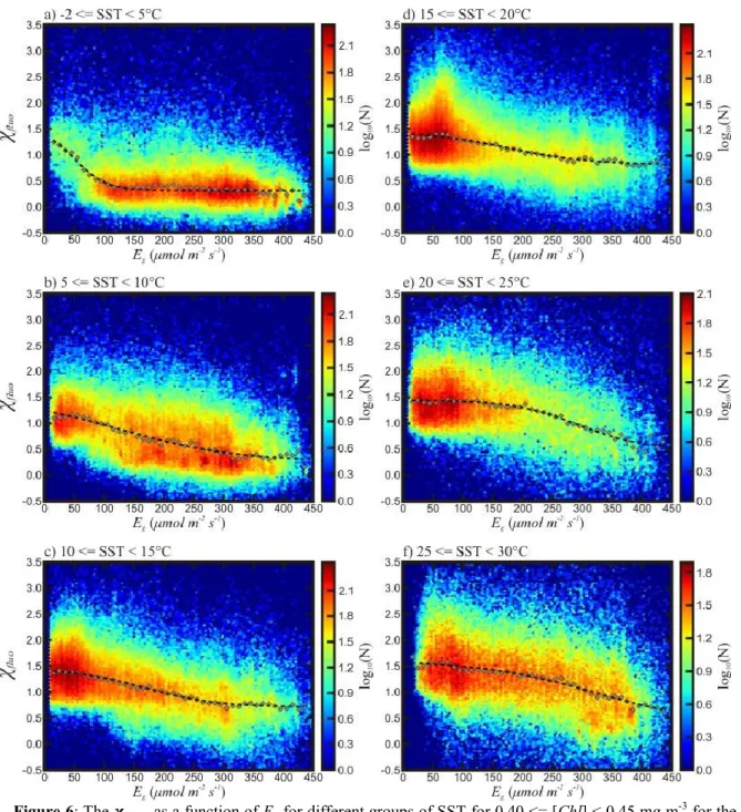
Figure 6: The 𝝌𝒇𝒍𝒖𝒐 as a function of Eg for different groups of SST for 0.40 <= [Chl] < 0.45 mg m-3 for the months

of May to September 2006. The colors represent the logarithm in base 10 of the number of points. The grey points are a representation of the median 𝝌𝒇𝒍𝒖𝒐 for 10 μmol m-2 s-1 intervals in Eg. The dashed line is the negated translated

sigmoidal function that best approximates the median values (see Figure 4).

Grouping data based on SST also highlights the presence of the cold waters group

present below 10°C. At low SST, the relationship for [Chl] between 0.40 and 0.45 mg chl m-3

(Fig. 6a) has one main “floor” value when Eg is greater than ~100 μmol m-2 s-1. For lower Eg, the

~ 33 ~

small fraction of points are present in this region of low Eg. The transition between the cold waters group and warm waters group is apparent as SST increases (Fig. 6, Fig. 5b). Furthermore,

as SST increases, 𝜒𝑓𝑙𝑢𝑜 will generally tend to be higher. This is particularly evident between the

cold and warm waters groups at higher Eg. With increased SST, there is also an increase in 𝜒𝑓𝑙𝑢𝑜

variability (Fig. 3b). Warm waters tend to harbor lower concentration of phytoplankton where variability is greater.

The behavior of 𝜒_{𝑓𝑙𝑢𝑜} at higher temperature, which excludes the cold waters group (i.e.,

for 15 <= SST < 20°C; Fig. 4), is similar to that observed for all [Chl], but the standard deviation of the data to the median trend decreases as [Chl] increases (e.g.,  = 0.43 for 0.40 <= [Chl] < 0.45 mg chl m-3 and 15 <= SST < 20°C and  = 0.50 for 0.40 <= [Chl] < 0.45 mg chl m-3).

Generally, the warm waters group highlighted in the right column of Figure 4 shows that

Eg had a significant impact on 𝜒𝑓𝑙𝑢𝑜. However, the subgroups with [Chl] < 0.2 mg chl m-3 still

displayed high variability. Under these conditions, the results show a dispersion of  ~0.87

around the mean value of 𝜒_{𝑓𝑙𝑢𝑜} with very little dependence on Eg until ~300 μmol m-2 s-1. This

would seem to indicate that either SST and/or Eg has little effect on the 𝜒𝑓𝑙𝑢𝑜 behavior under conditions of low [Chl], or support the calculations of Huot et al. (2013) that fluorescence

measured by MODIS is not valid below ~0.1 mg chl m-3 as it is below the detection limit of the

instrument (Huot et al., 2013; Meister et Franz, 2011; see discussion). The latter is the more

likely explanation and even at higher values (up to probably ~0.2 mg chl m-3) the noise can still

be significant and hide relationships with other variables. As a result, the values for areas where