DOI 10.1515 / JNUM.2010.010 c
° de Gruyter 2010
Convergence analysis of finite element methods for
H
H
H
(div; Ω)
(div; Ω)
(div; Ω)-elliptic interface problems
R. HIPTMAIR∗, J. LI∗, and J. ZOU∗†
Received March 2, 2010
Abstract — In this article we analyze a finite element method for solving H(div; Ω)-elliptic interface problems in general three-dimensional Lipschitz domains with smooth material inter-faces. The continuous problems are discretized by means of lowest order H(div; Ω)-conforming finite elements of the first family (Raviart–Thomas or N´ed´elec face elements) on a family of unstructured oriented tetrahedral meshes. These resolve the smooth interface in the sense of sufficient approximation in terms of a parameterδ that quantifies the mismatch between the smooth interface and the finite element mesh. Optimal error estimates in the H(div; Ω)-norms are obtained for the first time. The analysis is based on a so-calledδ -strip argument, a new ex-tension theorem for H1(div)-functions across smooth interfaces, a novel non-standard interface-aware interpolation operator, and a perturbation argument for degrees of freedom in H(div; Ω)-conforming finite elements. Numerical tests are presented to verify the theoretical predictions and confirm the optimal order convergence of the numerical solution.
Keywords: H(div; Ω)-elliptic interface problems, finite element methods, face elements, con-vergence analysis
1. Introduction
Given a bounded domain Ω ⊂ R3 with a Lipschitz boundary, we assume
that the domain Ω consists of two subdomains Ω1 and Ω2, where Ω1⋐Ω,
Ω2:= Ω \ Ω1. The internal interfaceΓ := ∂ Ω1 is assumed to be sufficiently
smooth, namely, at least C2-smooth (see Fig. 1 for an illustration of the
geo-metric setting). We are concerned with solving the H(div; Ω)-elliptic interface ∗SAM, ETH, Z¨urich, CH-8092 Z¨urich, Switzerland
†Department of Mathematics, The Chinese University of Hong Kong, Shatin, N.T., Hong Kong. The work of this author was substantially supported by Hong Kong RGC grants (Project 404606 and Project 404407) and partially supported by CUHK Focused Investment Scheme 2008/2010
Ω Ω1
Ω2
n
Γ
Figure 1. An illustrative sketch of the setting of the problem. problem
−grad(χ divu) + β u = f in Ω (1.1)
with Dirichlet boundary condition
u· n = 0 on ∂ Ω (1.2)
and jump conditions on the interface
[n · u] = 0 on Γ (1.3)
[χ div u] = 0 on Γ (1.4)
where f∈ L2(Ω) is the source term, and n stands for a unit normal vector to the boundary∂ Ω1pointing intoΩ2. By[v] := v1− v2we denote the jump of
a function v across the interfaceΓ. For ease of exposition, we assume that the coefficient functionsχ and β are piecewise constant, i.e.
χ(x) = ½χ 1, x ∈ Ω1 χ2, x ∈ Ω2, β (x) = ½β 1, x ∈ Ω1 β2, x ∈ Ω2
where χi and βi, i= 1, 2, are positive constants. The more general case of
piecewise smooth uniformly positive coefficients in L∞(Ω) can be treated sim-ilarly with no essential difficulty by using techniques like local averaging in an element.
As a rule, H(div; Ω)-elliptic interface problems like (1.1)–(1.4) arise from the first-order system least-squares formulation of elliptic interface problem, or preconditioning for the mixed finite element using a gradient formulation of the Dirichlet problem (see, e.g., [2, 7, 12, 17, 26] and the references therein).
Finite element methods for H(div; Ω)-elliptic problems have been well stud-ied in [2, 14, 17]. Nevertheless, the discontinuity of the coefficients across the smooth interface creates additional challenges. First, the global regularity of the solution might be significantly lower than the local regularity in each sub-domain due to the jump of coefficients across the interface. Thus, the tech-niques used for traditional H(div; Ω)-finite element methods with full regular-ity are not applicable here. Second, we are confronted with the issues of how to approximate the smooth interface by the finite element mesh, how to define practical numerical quadrature for those elements partially cut through by the interface, and, last but not least, whether it is still possible to obtain optimal convergence order using the H(div; Ω)-conforming finite element method for
H(div; Ω)-elliptic interface problems? Below we address all these issues. Due to the practical relevance of interface problems in many engineer-ing and industrial applications, numerical solution methods for interface prob-lems have been investigated extensively. One may refer to the monograph [20] and the references therein for a history of the development in this research field. Numerous variants of finite element methods (FEMs) for classical el-liptic interface problems in H1(Ω)- and H(curl; Ω)-settings have been ex-tensively studied in the past few decades. Interested readers may refer to [3,4,6,9,13,16,18,19,24] . Nevertheless, to the best knowledge of the authors, there seems to exist no corresponding work on the convergence analysis of
H(div; Ω)-elliptic interface problems discretized by means of interface-aligned face elements.
This article completes the numerical analysis of conforming finite ele-ment methods for three important classes of elliptic interface problems, namely those set in H1(Ω), H(curl; Ω) and H(div; Ω). General higher order Lagrange finite element methods for H1(Ω)-elliptic interface problems were discussed in [19]. In this paper key tools and concepts like theδ -strip argument and the perturbed interpolation were first introduced. A crucial insight obtained in [19] was that the optimal convergence order depends not only on the mesh size but also on the mismatch between the interface and the mesh. Subsequently, in [16] we investigated H(curl; Ω)-elliptic interface problems using lowest or-der edge elements of the first family. We or-derived optimal oror-der convergence in the H(curl; Ω)-norm for the first time. We relied on novel techniques such as the generalization of the concept of perturbed interpolation to edge elements, an H1(curl; Ωi) extension theorem and what we dubbed a ‘pyramid argument’.
The main contribution of the current work is to derive optimal order con-vergence in the H(div; Ω)-norm for H(div; Ω)-elliptic interface problems us-ing lowest order Raviart–Thomas (or N´ed´elec) H(div; Ω)-conformus-ing finite elements [5, 22]. We follow the lines of [16], with new twists, entailed by the
‘more non-local’ nature of the degrees of freedom for H(div; Ω)-conforming (face) finite elements. Therefore, the analytical tools and techniques had to be adjusted. This led to:
• a new non-standard interface-aware face element based interpolant, which is shown to possess optimal approximation in the sense of the
H(div; Ω)-norm, see Subsection 2.4;
• a modified δ -strip argument for quantifying the relation of error estimate near the interface in terms of the mismatch parameter δ between the triangulation and the smooth interface, see Corollary 3.1;
• a new extension theorem for H1(div; Ω
i) functions across smooth
in-terfaces for i= 1, 2, which bridges the gap between standard and non-standard interpolation and thus is crucial for the convergence analysis, see Theorem 3.2;
• a perturbation argument for the degrees of freedom of H(div;Ω)-con-forming finite elements, see the proof of the pivotal Lemma 4.2.
The remainder of the paper is organized as follows: In Section 2, we first introduce some necessary notations and assumptions to be used later, then de-rive the variational formulation for the H(div; Ω)-elliptic interface problem, and propose a practical finite element approximation using the lowest order Raviart–Thomas finite element spaces. In Section 3 we establish some impor-tant auxiliary results, including a δ -strip argument for error estimation near the interface and the construction of a new extension operator for H1(div; Ωi)
functions across smooth interfaces for i= 1, 2. In Section 4, we prove optimal order convergence in the sense of H(div; Ω)-norm of the proposed finite ele-ment method for H(div; Ω)-elliptic interface problems. In Section 5, numerical experiments are presented to justify the theoretical prediction of the optimal convergence order. We summarize the work and point out future directions in Section 6.
2. Finite element approximation
We stick to the usual notations for Sobolev spaces H(div; Ω), H0(div; Ω), etc.,
see [12, Chap. 1] or [21]. We also write
H1(div; Ω) =©v∈ H1(Ω) | divv ∈ H1(Ω)ª.
2.1. Weak formulation
The weak formulation of (1.1)–(1.4) is straightforward and reads as follows.
Problem (Q). Seek u∈ H0(div; Ω) such that
a(u, v) =
Z
Ωf· vdx ∀ v ∈ H0(div; Ω) (2.1)
with the bilinear form defined by
a(u, v) := 2
∑
i=1 Z Ωi (χidiv ui· divvi+ βiui· vi) dx . (2.2)By the assumptions onχ and β in Section 1, the bilinear forms a(·,·) in (2.2) agrees with the H(div; Ω)-inner product of the Hilbert space H0(div; Ω) up to
the weightsχi’s andβi’s, and the associated energy norm
kuka= a(u, u)1/2 (2.3)
is equivalent to the H(div; Ω)-norm. This ensures the existence and uniqueness of the solution of (2.1) by the Lax–Milgram Lemma [10, Theorem 1.1.3].
Throughout the paper, we assume that the solution of (2.1) has the regular-ity H0(div; Ω) ∩ H1(div; Ω1) ∩ H1(div; Ω2), which is a natural assumption in
the present geometric setting.
2.2. Triangulations
Let the polyhedral domainΩ ∈ R3be equipped an oriented unstructured tetra-hedral meshes(Th)hin the sense of [15, Def. 3], where h stands for the
mesh-width. We denote by Fh, Eh and Nh the respective sets of oriented faces,
oriented edges and vertices of the triangulation Th. The quality of Th can
be gauged by means of its meshsize h := maxKhK, shape regularity measure
ρ(Th)and quasi-uniformity measure γ(Th) [8, Sect. 3] as follows
ρ(Th) := max K∈Th hK rK , h:= max K∈Th hK, γ(Th) := max K∈Th h hK where hK:= sup{|x − y| : x,y ∈ K} rK:= sup{r > 0 : ∃x ∈ K; |x − y| < r ⇒ y ∈ K}.
In the sequel, we will frequently denote by c and C generic positive constants which may depend on the domainΩ, the coefficientsχi’s, βi’s and the mesh
parametersρ(Th) and γ(Th), but must not depend on the meshwidth h and the
related functions.
In the remainder of this section, we shall illustrate our assumptions on the triangulation in relation to the interface. First of all, our finite element dis-cretization scheme relies heavily on the concept of interface-aware
triangula-tion, see [16, Ass. 2.1]:
Assumption 2.1 Interface-awareness. The triangulation This
interface-aware if for every K∈ Th all its four vertices are either inΩ1 or inΩ2, and
this element K is assumed to intersect with the interfaceΓ in such a way that
at most three of its vertices are located on the interfaceΓ while all remaining
vertices are either inΩ1or inΩ2.
Let us comment on Assumption 2.1 before we proceed. To meet the re-quirement of Assumption 2.1, the triangulation Th should not be too coarse
with respect to the interface, i.e., it is not allowed to have all the four ver-tices of an element K∈ Thlocated on the interfaceΓ. This might be the case
for some element on a rather coarse triangulation surrounded by the interface of large curvature. Nevertheless, we can always refine the mesh until all the elements satisfies Assumption 2.1 owing to the smoothness of the interface.
When an element K satisfies K∩ Γ 6= ∅, it is called an interface element, otherwise a non-interface element. The set of all interface elements is denoted by T∗:= {K ∈ Th|K ∩Γ 6= ∅} and T∗i:= {K ∈ T∗| all nodes of K are in Ωi}
represents the set of all interface elements of Ωi, i= 1, 2. For a fixed small
δ > 0, we define the δ -strip regions around the interface in Ω and Ωi, i= 1, 2,
respectively, by
Sδ := {x ∈ Ω| dist(x,Γ) < δ }, Sδi := {x ∈ Ωi| dist(x,Γ) < δ }, i = 1,2.
It is obvious that Sδ= S1δ∪S2δ∪Γ and T∗= T∗1∪T∗2, and theseδ -strip regions
will be used for the error estimate near the interface, which in general cannot be captured using the techniques of standard interpolation approximation. For a vivid illustration of the concepts above, readers may refer to Fig. 2 for a 2D scenario for better understanding.
According to Assumption 2.1, for any K ∈ T∗, it must intersect with the interfaceΓ in one and only one of the following three situations:
1. One vertex of K is located on the interfaceΓ, and the vertex located on the interface is called an interface vertex.
Ω Ω1 Ω2 n Γ K1 K2 K3 K4
Figure 2. Sδ: the region of width 2δ between the two closed dashed lines around the closed solid interface lineΓ. Interface elements: K3∈ T∗1, K4∈ T∗2. Non-interface elements: K1∈ T1,
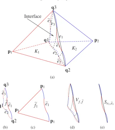
K2∈ T2. K1 K2 e1 e2 e3 q1 q2 q3 p1 p2 Interface (a) e1 e2 e3 q1 q2 q3 f (b) e1 q2 q3 p1 f1 (c)
Figure 3. (a): Two typical tetrahedral interface elements K1and K2intersect with the interface Γ. The interface are visualized by the intersected piecewise smooth curves composed of curved segments on the surfaces of the tetrahedra K1and K2. The interface edges are e1, e2and e3 denoted by straight (dashed) line segments; (b): An interface face f of the first kind; (c): An interface face f1of the second kind.
2. Two vertices of K are located on the interfaceΓ, and the oriented edge with two vertices on the interface is called an interface edge.
3. Three vertices of K are located on the interfaceΓ, and the triangular ori-ented face with three vertices on the interface is called an interface face
of the first kind, while the face with only two vertices on the interface is
called an interface face of the second kind.
And these notions are further illustrated by two typical interface elements in-tersecting the interface as shown in Fig. 3.
For the sake of discretization, the smooth interface Γ has to be approx-imately resolved by tetrahedral meshes. We quantify the quality of the
ap-proximation of the smooth interface Γ by the triangulation Th in terms of a
parameterδ through the following definition (see [16, Def. 2.2]).
Definition 2.1. The triangulation Th is said to resolve the interfaceΓ up
to an errorδ if it can be decomposed as
Th= T1∪ T2∪ T1 ∗ ∪ T∗2 where Ti= {K ∈ Th; K⊂ Ωi\ Sδ} and K∈ T∗iif max{dist(x,Γ ∩ K); x ∈ K ∩ Ωi′} 6 δ
for i= 1, 2, where we define i′= 1 if i = 2 and i′= 2 if i = 1.
We may refer to Fig. 2 for an illustration of Definition 2.1. It is worth re-marking that although we assume that all vertices of an element K must belong to either subdomainΩ1 orΩ2, it is allowed that the interface may cut some
elements into two parts lying in two different subdomains, see, for instance, triangle K4 in Fig. 2. By Definition 2.1 we easily see that any interface
ele-ment K can be embedded in the union of the interface strip Sδ and one of the subdomainsΩ1andΩ2.
For a smooth interface Γ approximated by a union of triangular faces of the triangulation Th, we may further quantify the parameterδ in terms of the
meshsize h as given by the next assumption.
Assumption 2.2. The interfaceΓ is C2-smooth. For the interface-aware
meshes, there exists some δ of order h2 for appropriately small h such that
K∩ Ω2⊂ S2δ for all elements K ∈ T∗1, and K∩ Ω1⊂ Sδ1 for all elements K∈
T2 ∗ .
A detailed proof of Assumption 2.2 of δ -approximation property for the interface-aware triangulation in two dimensions can be found in [9] using local coordinate system and the same idea can be easily extended to 3D with no essential changes.
For the subsequent error estimate, we will use a crucial perturbed inter-polation operator. To that end, we first introduce three more helpful auxiliary concepts aided with the sketches in Fig. 4.
Definition 2.2 (interface twin edge). For any oriented interface edge e1∈
K1 K2 e1 e e1 e2 e e2 e3 e e3 q1 q2 q3 p1 p2 Interface (a) e e1 e e2 e e3 q1 q2 q3 ef (b) e e1 p1 p1 p1 ef1 (c) Vf, ef (d) Se1,ee1 (e)
Figure 4. Illustration of interface twin edges and faces. (a): The interface twin edges areee1,ee2 andee3denoted by the piecewise smooth curves composed of curved segments on the interface; (b): An interface twin face efof the first kind; (c): An interface twin face ef1of the second kind; (d): small volume Vf, ef sandwiched by interface (twin) faces of first kind; (e): slim area Se1,ee1
enclosed by interface (twin) edges.
p1and p2, respectively, which share the interface edge e1and another interface
vertex q1, such that there is a unique oriented curveee1which is the intersection
of the interface and two triangular faces determined by p1with e1, and p2with
e1, respectively, and shares with e1 the same starting and end points. We call
e
e1the interface twin edge associated with e1(see Fig. 4a for an illustration).
It is emphasized that any interface edge is always a straight line segment, and the associated interface twin edge could be a piecewise smooth curve (see, e.g., the smooth curveee1 in Fig. 4a) which shares the two endpoints with the
interface edge e1.
Definition 2.3 (interface twin face of the first kind). For any oriented
Eh, with which three interface twin edges ee1,ee2,ee3 are associated, respec-tively, there exists a unique smooth surface ef on the interface circumscribed byee1,ee2,ee3. We call ef an interface twin face of the first kind associated with
the face f . The orientation of ef is determined in the sense that it approximates that of f as meshes refine (see Fig. 4b).
Definition 2.4 (interface twin face of the second kind). For any oriented
interface face of the second kind f1∈ Fhwith an interface edge e1∈ Eh, with
which the interface twin edgeee1 are associated, if f1 is an interface face of
an interface element K∈ T∗i, i= 1 or 2, then there exists a unique piecewise planar surface,
ef1= ( f1∪ Se1,ee1) \ Ωi′
with ‘\’ being understood as set minus operation. The orientation of ef1 is
determined in such a way that f1 and ef1 share the same orientation as f1 on
f1\ Se1,ee1 and ef1 extends this orientation on the other part Se1,ee1\ f1. We call
ef1 an interface twin face of the second kind associated with the face f1 (see
Fig. 4c).
For an oriented interface face of the second kind ficonsisting of one
inter-face edge ei ∈ Eh (with which the interface twin edgeseei are associated), we
will need the following set
Sei,eei= ( fi\ efi) ∪ ( efi\ fi)
which denotes the slim open piecewise planar surface set surrounded by the curves eiandeeifor i= 1, 2, 3 (see Fig. 4e).
For an interface face f of the first kind enclosed by three interface edges
e1, e2, e3∈ Eh, with which three interface twin edges ee1,ee2,ee3 are associated,
respectively, we denote by Vf, ef the closed volume set enclosed by the surfaces
f, ef, Se1,ee1, Se2,ee2 and Se3,ee3 (see Fig. 4d). It is readily to see by Assumption 2.2
that
Vf, ef ⊂ Sδ, Sei,eei⊂ Sδ, i= 1, 2, 3.
For the interface-aware triangulation, it is easy to deduce that |Vf, ef| ∼ δ h
2, |S
ei,eei| ∼ δ h (2.4)
where| · | represents either volume or area measures.
In the sequel, the triangulation Thwill be assumed to be sufficiently fine
geometry the interface twin edges might not be well defined for certain coarse meshes. But due to the C2-smoothness of the interface, we can always refine the mesh till a desired interface twin edge (resp. the associated interface twin face) is obtained for any interface edge.
2.3. Finite element discretization
A suitable trial space Fh⊂ H0(div; Ω) for the Galerkin discretization of (2.1)
is supplied by the lowest order Raviart–Thomas elements of the first family (see, e.g., [5, 22]), that is,
Fh:= © vh∈ H0(div; Ω) | vh|K(x) = aK+ bKx, aK∈ R3, bK∈ R, x ∈ K ∀K ∈ Th ª . Writing cFhfor the set of all interior faces of Th, the degrees of freedom of Fh are given by the surface integrals
vh7→
Z
f
vh· n dS , f ∈ cFh.
It is well established that there exists a well-defined global finite element inter-polation operatorΠh: H1(div; Ω) 7→ Fh(cf. [21, Thm. 5.25, Sect. 5.4]), which
has the following approximation property.
Lemma 2.1. The interpolation operatorΠhpossesses the optimal
approx-imation property
∃C = C(ρ(Th)) : ku − ΠhukH(div;Ω)6ChkukH1(div;Ω) ∀ u ∈ H1(div; Ω).
(2.5) Moreover, we recall that face elements are an affine equivalent family of finite elements with respect to the pullback transformation (see [15, 21])
Bbv(bx) := det(B)v(x) , x = Bbx+ t, B ∈ R3,3, t∈ R3. (2.6) On a tetrahedron K with vertices[a1, a2, a3, a4] and barycentric coordinates
λ1, λ2, λ3, λ4, the local shape function associated with a face f = [ai, aj, ak] are
given by (see [15, Sect. 3.2])
bKf = 2¡λigradλj× gradλk+ λjgradλk× gradλi
They can be assembled into a collection of global bases{bi, i = 1, . . . , ♯ cFh}
of Fh.
The following lemma can be shown by adapting the proof of Lemma 3.12 from [15] to bound the local basis functions in terms of the mesh size h.
Lemma 2.2. Let Thbe a quasi-uniform, oriented unstructured tetrahedral
mesh inΩ with meshsize h. Then there exist some positive constants C such that
the local basis functions bKf, f ⊂ ∂ K, satisfy the following error estimates
kbKfk2H(div;K)6 C h, kdivb f Kk2H(div;K)6 C h3. (2.8)
With the finite element function spaces presented above, the finite element approximation of (2.1) can be stated as follows.
Problem (Qhhh). Seek uh∈ Fhsuch that
a(uh, vh) =
Z
Ωf· vhdx ∀ vh∈ Fh. (2.9)
The existence and uniqueness of the solution of (2.9) follow from the Lax–Milgram lemma [10, Theorem 1.1.3], similar to those of the continuous Problem (Q). One natural idea to derive the estimate of discretization error is through the best approximation error estimate in light of the quasi-optimality from Cea’s lemma. But this is only possible, if the Galerkin matrix is computed exactly.
The exact evaluation of the stiffness matrix associated with the bilinear form a(·,·) in (2.9) can be very complicated on an interface element when it is cut through by the interface, especially in three dimensions. A much more convenient formulation is obtained by replacing the original bilinear form (2.2) with an approximate bilinear form ah(·,·):
ah(uh, vh) =
∑
K∈T
Z
K(χKdiv uh· divvh+ βK
uh· vh) dx (2.10)
where the coefficientsχK’s andβK’s are elementwise constant. In our present
setting of piecewise constant coefficients, for every K∈ T , χK= χi(βK= βi,
respectively) if K∈ Tior Ti
∗ for i∈ {1,2}.
With the modified bilinear form in (2.10), we can now define a more prac-tical finite element method for the variational Problem (Q) by replacing a(·,·) by ah(·,·).
Problem ( eQhhh). Find uh∈ Fhsuch that
ah(uh, vh) =
Z
It can be immediately seen that the bilinear form ah(·,·) still preserves
coercivity and continuity, and thus the well-posedness of Problem (eQh) is
as-sured. Moreover, the two bilinear forms ahand a are related to each other by a(u, v) = ah(u, v) + a∆(u, v) (2.12)
where the residual bilinear form a∆(·,·) satisfies
|a∆(u, v)| 6 CkukH(div;Sδ)kvkH(div;Sδ) (2.13)
with the constant C depending only on the coefficientsχi’s andβi’s.
2.4. Interface-aware interpolation operator
The modification of the bilinear form for ease of computation of stiffness matrix complicates the error estimate quite a lot. We have to recover quasi-optimality by taking into account numerical crime. It is worth remarking that there are no ambiguities of the interpolation operator Πh when applied for
functions in H0(div; Ω) ∩ H1(div; Ω1) ∩ H1(div; Ω2), but the corresponding
interpolant is not a good candidate to yield best approximation error esti-mate. It is worth pointing out that the original idea to derive error estimate by combining Cea’s lemma with interpolation error estimate of Πh, which
works in H(div; Ω)-elliptic problems, fails in H(div; Ω)-elliptic interface one. Instead we shall define a problem-specific interface-aware interpolation oper-ator, which can be viewed as a perturbed version of Πh. The pivotal idea is
to define a perturbed degree of freedom for each interface face of an interface element by a surrogate degree of freedom defined through the interface twin face. To be more precise, we elucidate the idea in the following definition, cf. [16, Sect. 2.4].
Definition 2.5 (interface-aware interpolation operators). Let Th be an
oriented unstructured tetrahedral triangulation satisfying Assumptions 2.1 and 2.2 with mesh size h, and Fhthe lowest order Raviart–Thomas elements on Th.
For a function u∈ H0(div; Ω) ∩ H1(div; Ω1) ∩ H1(div; Ω2), we define a
perturbedinterface-aware interpolation operator
e
Πh: H0(div; Ω) ∩ H1(div; Ω1) ∩ H1(div; Ω2) 7→ Fh
and its interpolation eΠhas follows:
Z f e Πhu· n dS = Z f u· n dS, f∈ Fhis a non-interface face Z
efu· n dS, f∈ Fhis an interface face associated
We remark that the interface-aware interpolation operator eΠhis introduced
only for the subsequent theoretical error estimates, and it is not needed in the numerical implementation of the finite element method(eQh).
3. Theoretical tools
In this section, we supply some technical results which are indispensable tools for the subsequent convergence analysis of finite element methods for
H(div; Ω)-elliptic interface problems.
We first recall an important inequality, under the same problem setting as in Section 1, which will be used for the error estimate in the region near the smooth interface. The proof is similar to that of [19, Lemma 2.1].
Lemma 3.1. Let i∈ {1,2}. Then it holds for any zi∈ H1(Ωi) that
kzikL2(Si
δ)6C
√
δ kzikH1(Ω
i)
provided thatδ is sufficiently small. Here the constant C depends only on the
smooth interface and the domainΩ.
There is a straightforward corollary to Lemma 3.1 which can be viewed as its vectorized version in H1(div) spaces by simply using the Cauchy–Schwarz inequality.
Corollary 3.1 (δδδ -strip argument). Let i ∈ {1,2}. Then it holds for any
zi∈ H1(div; Ωi) that kzikH(div;Si δ)6C √ δ kzikH1(div;Ω i)
provided that δ is sufficiently small. The constant C depends only on the smooth interface and the domainΩ.
Next, motivated by the construction of extension operators for functions in Sobolev spaces Hk(Ω) [1, 11], we develop in this subsection a new extension theorem for functions in the H1(div) space. This new extension result will play a crucial role in the subsequent error estimate on interface elements.
It is well-known that (see, e.g., [11, Theorem 1, Sec. 5.4]) for a connected bounded domain in U⊂ R3with C2-smooth boundary there exists a bounded
linear extension operator
such that for any scalar function u∈ H2(U): 1. Eu= u a.e. in U;
2. kEukH2(R3)6CkukH2(U)with the constant C depending only on U .
Compared with the extension of scalar functions, vector fields must be extended in a more delicate way to conserve their properties. In [16, Thm. 4.3], the following H1(curl)-extension theorem is proved based on the commuting diagram property [15]:
Ecurl(grad p) = grad(E p). (3.1)
Theorem 3.1 (H111(curl)-extension theorem). Assuming that U is a
con-nected bounded domain in R3 with C2-smooth boundary. Then there exists a
bounded linear extension operator:
Ecurl : H1(curl;U) → H1(curl; R3) (3.2)
such that for each u∈ H1(curl;U):
1. Ecurlu= u a.e. in U;
2. kEcurlukH1(curl;R3)6CkukH1(curl;U), with the constant C depending only
on U .
Analogously, suppose u∈ H1(div;U) and we wish to extend u to be a func-tioneu ∈ H1(div; R3). Since for a vector-valued function w ∈ H1(curl;U) we
have curl w∈ H1(div;U), it seems promising to define an H1(div)-extension
operator Edivstill based on the commuting diagram property [15]:
Ediv(curl w) = curl(Ecurlw). (3.3)
With such motivation, we are now able to show the H1(div)-extension theo-rem across the smooth boundary, whose proof will be given in detail in Ap-pendix A.
Theorem 3.2 (H111(div)-extension theorem). Assume that U is a connected
bounded domain in R3with C2-smooth boundary. Then there exists a bounded
linear extension operator:
Ediv: H1(div;U) → H1(div; R3), i= 1, 2 (3.4)
1. Edivu= u a.e. in U;
2. kEdivukH1(div;R3)6CkukH1(div;U), with the constant C depending only
on U .
For our subsequent analysis, we need the following special version of The-orem 3.2.
Corollary 3.2. There exist two bounded linear operators
Eidiv : H1(div; Ωi) → H1(div; Ω), i= 1, 2 (3.5)
such that for each u∈ H1(div; Ωi):
1. Eidivu= u a.e. in Ωi;
2. °°Eidivu°°H1(div;Ω)<∼ kukH1(div;Ω
i).
Proof. Noticing Assumption 2.2 that the interface Γ is C2-smooth, and
some slight modification in the proof of Theorem 3.2 immediately yields the
desired result. 2
The following inequality in a pyramid can be found in [16, Lemma 3.6], and will be applied to the error estimates in those pyramids with slender bottom faces in the next section.
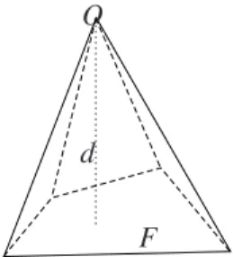
Lemma 3.2. Let P be a pyramid with F being its quadrilateral bottom
face and O its apex(see Fig. 5). Then we have
kuk2L2(F)6
3
dkukL2(P)(hPkgradukL2(P)+ kukL2(P)) ∀u ∈ H
1(P)
where d:= dist(O, F), hP:= max{|x − y| : x,y ∈ P}. Moreover, if d ∼ O(hP)
and hP< 1, we have kuk2L2(F)6C µ 1 hPkuk 2 L2(P)+ kgraduk2L2(P) ¶ ∀u ∈ H1(P) (3.6) with C> 0 independent of hP.
d F O
Figure 5. Sketch of the pyramid in Lemma 3.2.
4. Convergence analysis
In this section, we show the optimal convergence for the H(div)-elliptic in-terface problem using the lowest order H(div; Ω)-conforming finite element approximation. We first state a technical lemma to be used for the convergence theorem.
Lemma 4.1. Let u∈ H0(div; Ω) ∩ H1(div; Ω1) ∩ H1(div; Ω2). Then we
have
∑
K∈T1 ∗ kE1divu1k2H(div;K∩Ω2) 6 kE 1 divu1k2H(div;S2 δ) 6Cδ ku1k2H1(div;Ω 1) (4.1)∑
K∈T1 ∗ ku2k2H(div;K∩Ω2) 6 ku2k2H(div;S2 δ) 6Cδ ku2k2H1(div;Ω 2). (4.2) Analogously,∑
K∈T2 ∗ kE2divu2k2H(div;K∩Ω1) 6 kE 2 divu2k2H(div;S1 δ) 6Cδ ku2k2H1(div;Ω 2) (4.3)∑
K∈T2 ∗ ku1k2H(div;K∩Ω1) 6 ku1k2H(div;S1 δ) 6Cδ ku1k2H1(div;Ω 1). (4.4)Proof. We only prove (4.1)–(4.2) since the estimates (4.3)–(4.4) can be
shown in exactly the same manner. To see (4.1), we noteSK∈T1
∗ K∩ Ω2⊂ S
2
δ and that all elements of Th are pairwise disjoint, the first inequality in (4.1)
follows immediately from Assumption 2.2. For the second estimate, using the Corollary 3.1 and the continuity property of the extension operator E1divyields
kE1 divu1k2H(div;S2 δ) 6Cδ kE1divu1k2H1(div;Ω 2)6Cδ ku1k 2 H1(div;Ω1).
The estimate (4.2) is obtained analogously by noting the fact thatSK∈T1 ∗ K∩
To obtain the convergence result, we need to show an appropriate interpo-lation error estimate for the interface-aware interpointerpo-lation operator eΠhin
Defi-nition 2.5. The following estimate is the counterpart of [16, Lemma 4.2], with a much more involved proof, however, due to more complicated geometrical considerations.
Lemma 4.2. Let u∈ H0(div; Ω) ∩ H1(div; Ω1) ∩ H1(div; Ω2). Then we
have ° ° °u − eΠhu ° ° ° H(div;Ω)6C µ h+√δ +√δ h ¶³ kukH1(div;Ω 1)+kukH1(div;Ω2) ´ (4.5)
with constant C> 0 depending on ρ(Th), γ(Th) and Ω, but independent of h,
δ and u.
Proof. Let K∈ T∗1. We notice the crucial identity is
e Πhu ¯ ¯ ¯ K= eΠhE 1 divu ¯ ¯ ¯ K.
Then we can decompose the difference u− eΠhu over K into three parts:
³
u− eΠhu´¯¯¯
K =
¡
u− E1divu¢¯¯K+¡E1divu− ΠhE1divu¢¯¯K
+³ΠhE1divu− eΠhE1divu´¯¯¯
K. (4.6)
Noting that u= E1
divu on K∩ Ω1and employing Lemma 4.1 leads to
∑
K∈T1 ∗ ° °u −E1 divu ° °2 H(div;K)=∑
K∈T1 ∗ ° °u −E1 divu ° °2 H(div;K∩Ω2) 6C∑
K∈T1 ∗ kuk2H(div;K∩Ω2)+∑
K∈T1 ∗ ° °E1 divu ° °2 H(div;K∩Ω2) 6Cδ kuk2H1(div;Ω 1). (4.7)stan-e1 e2 e3 f n (a) e e1 e e2 e e3 ef n (b) Figure 6. Orientations of interface (twin) faces.
dard interpolation operatorΠhand the continuous property of E1divgive
∑
K∈T1 ∗ ° °E1 divu− ΠhE1divu ° °2 H(div;K)6C∑
K∈T1 ∗h2°°E1divu°°2H1(div;K)
6Ch2°°E1divu°°H21(div;Ω)6Ch2kuk2H1(div;Ω
1). (4.8)
The most challenging issue comes from the third term in the right hand side of (4.6), where we observe that the only difference between two interpolation functions involved lies in the degrees of freedom associated with the interface faces of first and second kind. Without loss of generality, let us consider a typical case, namely picking up the interface element K1 as shown in Fig. 4a
as our current K and assuming that most part of K1lies inΩ1.
We shall investigate the error estimate in K1 in detail step by step with
reference to Fig. 4. First of all, we have by the definition ofΠhand eΠh:
° ° °ΠhE1divu − eΠhE1divu ° ° °2H (div;K1) = ° ° ° ° µZ f E1divu· d~S − Z efE 1 divu· d~S ¶ bf + 3
∑
i=1 µZ fi E1divu· d~S − Z efi E1divu· d~S ¶ bfi ° ° ° ° 2 H(div;K1) .Without loss of generality, all basis functions bfi, i= 1, 2, 3, and bf refer to
outgoing fluxes with normal vectors pointing outward. Here we play the trick to enclose Vf, ef by adding Sei,eei, i= 1, 2, 3, to f and − ef (which means ef with opposite orientation) and subtracting the surplus. Note that for h sufficiently small, the orientations of f and ef are approximately the same as indicated by the outward normal direction n in Figs. 6a and 6b. Note that the orientations of
Then the equality above can be rewritten as the following crucial identity: ° ° ° ° µZ f E1divu· d~S − Z efE 1 divu· d~S ¶ bf + 3
∑
i=1 µZ fi E1divu· d~S − Z efi E1divu· d~S ¶ bfi ° ° ° ° 2 H(div;K1) = ° ° ° ° µZf∪(− ef)∪Se1,ee1∪Se2,ee2∪Se3,ee3
E1divu· d~S ¶ bf + 3
∑
i=1 µZ Sei,eei E1divu· d~S ¶ (bfi− bf) ° ° ° ° 2 H(div;K1) :=°°Θ + Λ°°2H(div;K 1).An insightful observation of the orientations of f , ef, Se1,ee1, Se2,ee2 and Se3,ee3
enables us to apply the divergence law to further estimateΘ: kΘk2H(div;K1)6C ° °bf ° °2 H(div;K1) ÃZ Vf, ef div E1divu dV !2 6C 1 h3 ÃZ Vf, ef div E1divu dV !2 6C|Vf, ef| h3 ÃZ Vf, ef|divE 1 divu|2dV !
where we employ the H(div)-estimates for the basis function bf in Lemma 2.2
in the second inequality and use the Cauchy–Schwarz inequality in the third one.
Another important observation is the following divergence-free property: div(bf1
K − b
f2
K) = 0 (4.9)
where f1, f2are two different faces of any tetrahedron K with the same
orien-tation, i.e., both pointing either inward or outward with respect to K. With this in mind, we now estimateΛ as follows:
kΛk2H(div;K1)6C 3
∑
i=1 ° °(bfi− bf) ° °2 L2(K 1) ÃZ Sei,eei E1divu· d~S !2 6C 3∑
i=1 ³° °bfi ° ° L2(K 1)+ ° °bf ° °2 L2(K 1) ´ÃZ Sei,eei E1divu· d~S !2 6C|Se,ee| h µZ Se,ee |E1divu|2dS ¶where we employ the L2-estimates for the basis function bf bfi in Lemma 2.2
and use the Cauchy–Schwarz inequality in the last inequality.
It is pointed out that the local error estimate above is done within an ele-ment. The same argument can be applied for any element patch by combining
K1 with adjacent interface elements with no interface face of the first kind.
Hence taking summation over all the interface faces and noticing that all slen-der volumes corresponding to the interface faces of the first kind are restricted in theδ -region with finite overlap due to the quasi-uniformity assumption of the triangulation, i.e.,
[ f∈Fh f⊂Sδ Vf, ef ⊂ Sδ (4.10) thus we obtain
∑
K∈T1 ∗ ° ° °ΠhE1divu− eΠhE1divu ° ° °2H(div;K) < ∼∑
K∈T1 ∗ Ã∑
f∈Fh f⊂K∩Sδ |Vf, ef| h3 ÃZ Vf, ef|divE 1 divu|2dV ! +∑
e∈Eh e⊂K∩Sδ |Se,ee| h µZ Se,ee |E1 divu|2dS ¶! < ∼ δ h ° °divE1 divu ° °2 L2(Sδ)+ δ h ° °E1 divu ° °2 L2(Sδ)+ δ ° °gradE1 divu ° °2 L2(Sδ) < ∼ µδ2 h + δ ¶ kuk2H1(div;Ω 1). (4.11)Here we substitute (2.4) into the first inequality, make use of the inclusion (4.10) and apply Lemma 3.2 in the second one, and finally employ theδ -strip argument (Corollary 3.1) together with the continuity of the extension operator
E1divin the last one.
Now for any non-interface element K∈ T1, u∈ H1(div; K) and u− eΠhu=
u− Πhu. Again a classical interpolation result (cf. [21]) yields
∑
K∈T1 ° ° °u − eΠhu ° ° °2 H(div;K) =∑
K∈T1 ku − Πhuk2H(div;K) < ∼∑
K∈T1h2kuk2H1(div;K)<∼h2kuk2H1(div;Ω
Combining (4.6), (4.7), (4.8), (4.11), and (4.12) yields
∑
K∈T1∪T1 ∗ ° ° °u − eΠhu ° ° °2 H(div;K) < ∼ µ δ2 h + δ + h 2 ¶ kuk2H1(div;Ω1). (4.13)Completely analogously, we repeat the previous argument by interchang-ing the indices from 1 to 2 and arrive at the error estimate for any K∈ T2∪T∗2. The desired error estimate results from combining the two parts of
contribu-tion, which completes our proof. 2
Now we are in a position to state our main theorem about the optimal con-vergence of Galerkin solutions of H(div)-elliptic interface problems by face elements.
Theorem 4.1. Let u and uh be the solutions to Problems (Q) and (eQh),
respectively, and assume u∈ H0(div; Ω) ∩H1(div; Ω1) ∩H1(div; Ω2). Then we
have the following error estimate under Assumptions2.1 and 2.2:
ku − uhkH(div;Ω)6Ch(kukH1(div;Ω1)+kukH1(div;Ω2)) (4.14)
with constant C> 0 depending on χi’s, βi’s,ρ(Th), γ(Th) and Ω, but
inde-pendent of h,δ and u.
Proof. We apply the first Strang lemma (see, e.g., [10], Theorem 4.1.1) to
(2.9) and (2.11) ku − uhkH(div;Ω)6C inf wh∈Fh ½ ku − whkH(div;Ω)+ sup vh∈Fh |a(wh, vh) − ah(wh, vh)| kvhkH(div;Ω) ¾ . (4.15) In particular, we choose wh= eΠhu. By Lemma 4.2 we have
ku − eΠhukH(div;Ω)6C µ δ √ h+ h + √ 䶳kukH1(div;Ω 1)+kukH1(div;Ω2) ´ . (4.16) Next, for any vh∈ Fhwe can derive by using Lemma 4.1 and Corollary 3.1
that
|a∆( eΠhu, vh)| 6 CkeΠhukH(div;Sδ)kvhkH(div;Sδ)
6C³kukH(div;Sδ)+ ku − eΠhukH(div;Sδ)
´ kvhkH(div;Sδ) 6Cµ√δ + h +√δ h ¶³ kukH1(div;Ω 1)+kukH1(div;Ω2) ´ kvhkH(div;Ω)
which implies that sup v∈Fh |a∆( eΠhu, vh)| kvhkH(div;Ω) 6Cµ√δ + h +√δ h ¶³ kukH1(div;Ω 1)+kukH1(div;Ω2) ´ . (4.17) The desired estimate now follows from Assumption 2.2 by substituting δ ∼ O(h2) into wherever δ occurs in (4.15)–(4.17) and plugging (4.16)–(4.17) into
(4.15). 2
Remark 4.1. The optimal convergence result in Theorem 4.1 does not
ad-dress the impact of coefficients, which is implicitly taken into account in the generic constant C. Actually the relative size ratio of coefficients could have enormous effect in the numerical computation, especially when it is extremely large or small. This issue is beyond the scope of our current work and will be addressed in the future.
5. Numerical experiments
In this section, we conduct numerical test to verify the theoretical prediction of the convergence analysis developed in previous sections. Our numerical exper-iments are implemented using Matlab combined with the commercial package Femlab. We will test the first family of N´ed´elec face elements of the lowest order. It is remarked that we use non-nested families of triangulations in order to make sure they are interface-aware. Note that after each step of mesh refine-ment, some regularly refined interface elements have to be slightly adjusted to meet the interface-aware condition. In the sequel, we will test the convergence rates for the relative error in the H(div; Ω)-norm which is defined by
Relative H(div; Ω) error :=ku − uhkH(div;Ω) kukH(div;Ω)
(5.1)
and relative error in the energy norm, namely,
Relative energy error := ku − uhka kuka
. (5.2)
Note that both H(div; Ω) and energy norms are numerically computed using a fourth order quadrature rule.
Example 5.1. The computational domain is taken to be a ballΩ = {(x,y,z):
x2+ y2+ z26r
z2= r1}. The exact solution u(x,y,z) is given by u(x, y, z) = 1 χ1 u1(x, y, z), x2+ y2+ z26r1 1 χ2 u2(x, y, z), r1< x2+ y2+ z26r2 (5.3) where u1(x, y, z) is given by (y − z) + n1(r21− x2− y2)(z − x) − n1(r12− x2− y2)(x − y) −n1(r12− x2− y2)(y − z) + (z − x) + n1(r21− x2− y2)(x − y) n1(r21− x2− y2)(y − z) − n1(r12− x2− y2)(z − x) + (x − y) and u2(x, y, z) by (y − z) + n2(r21− x2− y2)(r22− x2− y2)(z − x) −n2(r21− x2− y2)(r22− x2− y2)(x − y) −n2(r12− x2− y2)(r22− x2− y2)(y − z) + (z − x) +n2(r21− x2− y2)(r22− x2− y2)(x − y) n2(r21− x2− y2)(r22− x2− y2)(y − z) −n2(r21− x2− y2)(r22− x2− y2)(z − x) + (x − y) .
For this example, we fix r1= 1, r2= 2, n2= 20, n1= n2(r22−r12), β1= β2=
1 and derive the source functions f through the equation (1.1) for different pairs
10−0.9 10−0.5 10−0.1 100.3 10−2 10−1 100 Meshsize [log] Relative H(div, Ω ) error [log] error O(h) (a) 10−0.9 10−0.5 10−0.1 100.3 10−2 10−1 100 Meshsize [log] Relative H(div, Ω ) error [log] error O(h) (b) 10−0.9 10−0.5 10−0.1 100.3 10−2 10−1 100 Meshsize [log] Relative H(div, Ω ) error [log] error O(h) (c)
Figure 8. The convergence rates for: (a)χ1= 1, χ2= 10; (b) χ1= 1, χ2= 103; and (c)χ1= 1, χ2= 10−3, respectively.
10−8 10−6 10−4 10−2 100 102 104 106 108
10−2
10−1
100
Jump ratio [log]
Relative energy error [log]
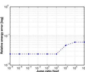
Figure 9. Relative error in the energy norm versus relative jump of coefficients for a fine trian-gulation with meshsize h= 0.1232 in Example5.1.
ofχ1 andχ2, using the exact solution (5.3) which satisfies the homogeneous
boundary condition and jump conditions on the interface. Numerical conver-gence tests are carried out to analyze the rates of the error decay using lowest order face elements of the first family. We start our tests on a rather coarse mesh with maximum mesh size h= 2 and then refine the mesh in a regular and uniform way which subdivides a coarse element into eight smaller ones. The refinement process will be done for three consecutive times which amounts to 2, 568, 192 degrees of freedom at the finest mesh with mesh size h = 0.125.
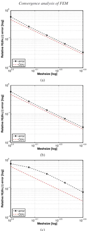
A slice view of the interface-aware mesh are shown in Fig. 7. From Fig. 8a with χ1 = 1 and χ2 = 10, it can be clearly seen that as the mesh gets finer
and finer, the line of the convergence rate tends to be parallel to the reference line of first order convergence in terms of the mesh size. More precisely, in the asymptotic sense, face elements indeed yield the optimal first order con-vergence in the H(div; Ω) norm as predicted by theory. Next, we adjust the relative jump of the coefficientsχ2/χ1to be 103 and 10−3, respectively, and
also plot the corresponding convergence rates in Figs. 8b and 8c. Similar obser-vations with asymptotic tendency of first order convergence rate with respect to the meshsize further consolidate our theoretical result.
Last, we test the relation between the relative error in the energy norm and relative jump of the coefficientsχ2/χ1. On a typical fine mesh with mesh size
h= 0.1232 with 4,396,225 degrees of freedom. We increase the relative jump of coefficients from 10−8 to 108 by fixing χ1 or χ2 to be unity and plot the
corresponding relative energy error curve versus the relative jump in Fig. 9. It can be seen that the numerical solution converges quite robustly in the sense of energy norm with respect to the relative jump of coefficients.
6. Conclusion
We have analyzed the convergence of the H(div; Ω)-conforming finite ele-ment method for H(div; Ω)-elliptic interface problems based on families of interface-aligned meshes. The difficulty mainly arises from the discontinuity of the coefficient in the second order term of equation (1.1). Optimal conver-gence results in H(div; Ω)-norm are obtained under reasonable regularity as-sumptions. With this work, we have completed the finite element convergence analysis for standard second order elliptic interface problems [19], H(curl; Ω)-elliptic interface problems [16] and H(div; Ω)-Ω)-elliptic interface problems (this work). Optimal rates can be established for each case.
Appendix A
Proof of Theorem 3.2. 1. We first prove the half ball extension
follow-ing [1, 25].
For a fixed x0∈ Γ, we first suppose that ∂U is flat near x0which is lying in the plane{x | x3= 0}. We assume that there exists an open ball
B= {x;|x − x0| < r}
with center x0and radius r> 0 such that ½
B+:= B ∩ {x3>0} ⊂ U,
B−:= B ∩ {x3< 0} ⊂ R3\U.
2. Suppose p∈ C∞(U). We define a H1(curl) reflection of p from B+ to
B−: ep = p(x), x∈ B+
∑
3j=1λjp 1¡x 1, x2, − x3 j ¢∑
3j=1λjp 2¡x 1, x2, − x3 j ¢∑
3j=1− λj j p 3¡x 1, x2, − x3 j ¢ , x ∈ B− (A.1)where(λ1, λ2, λ3) are the solutions of the 3 × 3 system of linear equations 3
∑
j=1 µ −1j ¶k λj= 1, k= 0, 1, 2 (A.2)which has the unique solution(λ1, λ2, λ3) = (6, −32,27). It is readily checked
that
ep ∈ C1(B).
Now we define a reflection of curl p from B+to B−in view of (3.3). ^
curl p=
½
curl p, x ∈ B+
curlep, x ∈ B− (A.3)
or ^ curl p= p3x2− p2x3 p1x3− p3x1 p2x1− p1x2 , x∈ B+
∑
3j=1− λj j p 3 x2 ¡ x1, x2, − x3 j ¢ −∑
3j=1− λj j p 2 x3 ¡ x1, x2, − x3 j ¢∑
3j=1− λj j p 1 x3 ¡ x1, x2, − x3 j ¢ −∑
3j=1− λj j p 3 x1 ¡ x1, x2, − x3 j ¢∑
3j=1λjp 2 x1 ¡ x1, x2, − x3 j ¢ −∑
3j=1λjp 1 x2 ¡ x1, x2, − x3 j ¢ , x ∈ B−. (A.4)Comparing the components of ^curl p in (A.4) in B+ and B−, we derive a tentative extension formula for a vector-valued function w= (w1, w2, w3)t ∈
C∞(B+) as follows: e w(x) = f w1(x) f w2(x) f w3(x) := w(x), x∈ B+
∑
3j=1− λj jw 1¡x 1, x2, − x3 j ¢∑
3j=1− λj jw 2¡x 1, x2, − x3 j ¢∑
3j=1λjw 3¡x 1, x2, − x3 j ¢ , x ∈ B−. (A.5)3. We claimwe∈ C1(B) and thus divwe∈ C0(B). This can be demonstrated by a detailed computation. Indeed according to (A.5) and (A.2),
lim x3→0+ e wi(x) = lim x3→0− e wi(x), i= 1, 2, 3 (A.6) lim x3→0+ e wi xj(x) = lim x3→0− e wi xj(x), i, j = 1, 2, 3. (A.7) 4. We prove
kewkH1(div;B)6CkwkH1(div;B+). (A.8)
In fact, by the definition ofw we can derivee
Z B|e w(x)|2dx = Z B+|w(x)| 2dx+Z B− ¯ ¯ ¯ ¯
∑
3j=1 λj − jw 1 µ x1, x2, − x3 j ¶¯¯¯ ¯ 2 dx + Z B− ¯ ¯ ¯ ¯∑
3j=1 λj − jw 2 µ x1, x2, − x3 j ¶¯¯¯ ¯ 2 dx + Z B− ¯ ¯ ¯ ¯∑
3j=1λjw 3 µ x1, x2, − x3 j ¶¯¯¯ ¯ 2 dx 6 C Z B+|w(x)| 2dx Z B|grad e w(x)|2dx = 3∑
i=1 3∑
k=1 Z B+|w i xk(x)| 2dx + 3∑
k=1 Z B− ¯ ¯ ¯ ¯∑
3 j=1 λj − jw 1 xk µ x1, x2, − x3 j ¶¯¯¯ ¯ 2 dx + 3∑
k=1 Z B− ¯ ¯ ¯ ¯∑
3 j=1 λj − jw 2 xk µ x1, x2, − x3 j ¶¯¯¯ ¯ 2 dx + 3∑
k=1 Z B− ¯ ¯ ¯ ¯∑
3j=1λjw 3 xk µ x1, x2, − x3 j ¶¯¯¯ ¯ 2 dx 6 C Z B+|gradw(x)| 2dxZ B|div e w(x)|2dx = Z B+|w 1 x1(x) + w 2 x2(x) + w 3 x3(x)| 2dx + Z B− ¯ ¯ ¯
∑
3j=1 λj − jw 1 x1 ³ x1, x2, − x3 j ´ +∑
3j=1 λj − jw 2 x2 ³ x1, x2, − x3 j ´ +∑
3j=1 λj − jw 3 x3 ³ x1, x2, − x3 j ´¯¯¯2 dx 6C Z B+|divw(x)| 2dx Z B|graddiv e w(x)|2dx = 3∑
k=1 Z B+|w 1 x1,xk(x) + w 2 x2,xk(x) + w 3 x3,xk(x)| 2dx + 3∑
k=1 Z B− ¯ ¯ ¯∑
3j=1 λj − jw 1 x1,xk ³ x1, x2, − x3 j⌊(k+1)/2⌋ ´ +∑
3j=1 λj − jw 2 x2,xk ³ x1, x2, − x3 j⌊(k+1)/2⌋ ´ +∑
3j=1 λj − jw 3 x3,xk ³ x1, x2, − x3 j⌊(k+1)/2⌋ ´¯¯¯2 dx 6 C Z B+|graddivw(x)| 2dx.The estimate (A.8) now follows readily from the above four inequalities. 5. If∂U is not flat near x0, we can find a C2-mappingΦ, with the inverse
Φ−1, such thatΦ flattens∂U near x0. We can write y= Φ(x), x = Φ−1(y), and
v(y) := w(Φ−1(y)). Choosing a small ball B and arguing as in the previous steps, we can extend v from B+ to a functionev defined in B such that ev ∈
C1(B) and thus curlev ∈ C0(B) and the following estimate holds for any v ∈
H1(div; B+):
kevkH1(div;B)6CkvkH1(div;B+). (A.9)
Letting W := Φ−1(B), W+:= Φ−1(B+) and converting back to the x-variable,
we have
kevkH1(div;W )6CkvkH1(div;W+). (A.10)
6. Due to the compactness of∂U, there exist finitely many open balls Wi, i= 1, 2, . . . , N, such that ∂U ⊂SNi=1Wi. Take W0⋐U such that U ⊂SNi=0Wi.
Let{ϑi}Ni=0be a partition of unity associated with Wi, i= 0, 1, 2, . . . , N. For any
given smooth w= ∑N
i=0wiwith wi= ϑiw, letwe= w0+ ∑Ni=1wei, whereweiare
extensions of wi defined in Wifor i= 1, 2, . . . , N. Replacingev and v in (A.10)
withweiand wi, respectively, and taking summation from 0 to N we obtain
kewkH1(div;R3)6CkwkH1(div;U) (A.11)
for some constant C depending on U but not on w. 7. Hereafter we define an extension operator
Edivw=we
and observe that the mapping w7→ Edivw is linear. Using the density of C∞(U)
in H1(div;U), we can verify that the operator Edivis what we desire.
This completes the proof of the theorem. 2
References
1. R. A. Adams, Sobolev Spaces. Academic Press, New York–London, 1975.
2. D. N. Arnold, R. S. Falk, and R. Winther, Preconditioning in H(div) and applications.
Math. Comp.(1997) 66, 957 – 984.
3. J. W. Barrett and C. M. Elliott, Fitted and unfitted finite-element methods for elliptic equa-tions with smooth interfaces. IMA J. Numer. Anal. (1987) 7, 283 – 300.
4. J. H. Bramble and J. T. King, A finite element method for interface problems in domains with smooth boundaries and interfaces. Adv. Comp. Math. (1996) 6, 109 – 138.
5. F. Brezzi and M. Fortin, Mixed and Hybrid Finite Element Methods. Springer-Verlag, New York, 1991.
6. E. Burman and P. Hansbo, Interior penalty stabilized Lagrange multiplier methods for the finite element solution of elliptic interface problems. IMA Numer. Anal. (accepted). 7. Z. Cai, R. Lazarov, T. Manteuffel, and S. McCormick, First-order system least-squares for
partial differential equations, Part I. SIAM J. Numer. Anal. (1994) 31, 1785 – 1799. 8. T. Chan and J. Zou, A convergence theory of multilevel additive Schwarz methods on
un-structured meshes. Numer. Algorithms (1996) 13, 365 – 398.
9. Z. Chen and J. Zou, Finite element methods and their convergence for elliptic and parabolic interface problems. Numer. Math. 79 (1998) 79, 175 – 202.
10. P. G. Ciarlet, The Finite Element Method for Elliptic Problems. Studies in Math. Appl., North-Holland Pub. Co., Amsterdam–New York, 1978.
11. L. C. Evans, Partial Differential Equations. Rhode Island : American Mathematical Soci-ety, Providence, 1998.
12. V. Girault and P. Raviart, Finite Element Methods for Navier–Stokes equations. Springer, Berlin, 1986.