Digital Image and Video Processing
Texte intégral
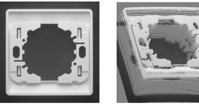
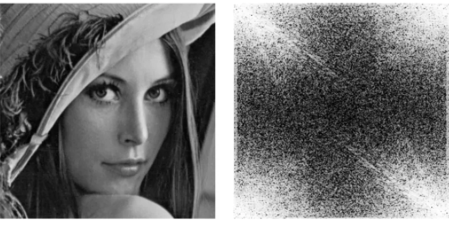
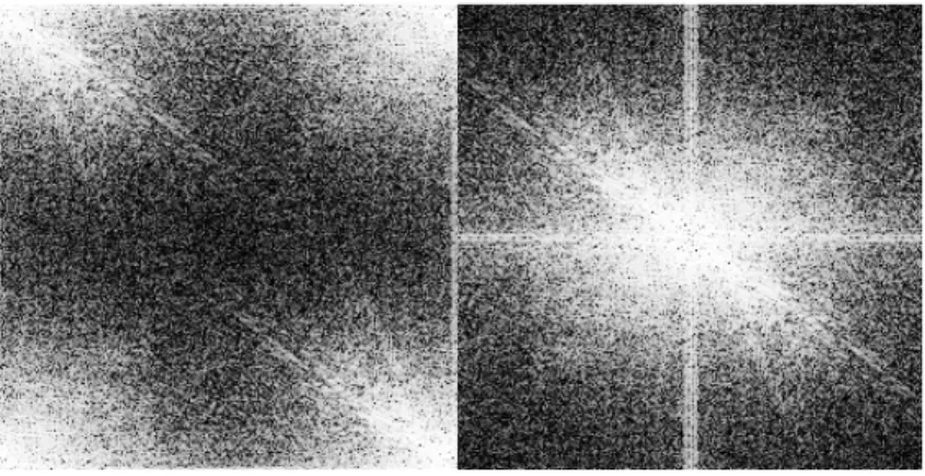
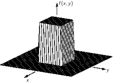
Figure
![Figure : Profile/cross-section of sensor. [Wikipedia]](https://thumb-eu.123doks.com/thumbv2/123doknet/6712289.184581/22.544.76.450.56.331/figure-profile-cross-section-of-sensor-wikipedia.webp)
Documents relatifs
The development of tools to support multilingual legislative drafting must draw on the broad technical areas of markup languages and hypertext, computer supported collaborative work
Avec ses 8000 membres répartis dans trente-neuf cercles fribourgeois disséminés dans notre pays - pour la plus grande partie en Suisse romande - il était dif¬. ficile pour
Glycosyl hydrolase family 1 Amino acid tRNA synthetase class I E and Q Homologous to ATPase AAA family Unknown function PPR repeats Homologous to calcineurin B Homologous
Although fundamental low-level features such as color, edge, texture, motion and stereo have reported reasonable success, recent visual applica- tions using mobile devices and
Et c’est pour cette raison que selon Richard Florida, le développement de l’économie locale passe par une manœuvre tout à fait judicieuse d’un point de vue économique :
on Which said scene is mapped in accordance With a ?rst projection associated With said ?rst point of sight, Wherein each source pixel has a point in said scene
The interface consists of (i) the input ports for the video signals (vblank, hblank, act video) and the video data, (ii) the output ports are equal to the number of the pixels of
1) Taking into account the relationship between HSI channels by calculating the correlation, constructing a linear predictor of the next channel value from the
