Three-dimensional flow past a fixed or freely vibrating cylinder in the early turbulent regime

Open Archive TOULOUSE Archive Ouverte (OATAO)

OATAO is an open access repository that collects the work of Toulouse researchers and

makes it freely available over the web where possible.

This is an author-deposited version published in:

http://oatao.univ-toulouse.fr/

Eprints ID : 19434

To link to this article

: DOI:10.1103/PhysRevFluids.3.013902

URL :

http://dx.doi.org/10.1103/PhysRevFluids.3.013902

To cite this version

:

Gsell, Simon and Bourguet, Rémi and Braza, Marianna.

Three-dimensional flow past a fixed or freely vibrating cylinder in the

early turbulent regime. (2018) Physical Review Fluids, vol. 3 (n° 1).

pp. 013902. ISSN 2470-0053

Three-dimensional flow past a fixed or freely vibrating cylinder

in the early turbulent regime

Simon Gsell, Rémi Bourguet,*_{and Marianna Braza}

Institut de Mécanique des Fluides de Toulouse, IMFT, Université de Toulouse, CNRS - Toulouse, France

(Received 24 July 2017; published 10 January 2018)

The three-dimensional structure of the flow downstream of a circular cylinder, either fixed or subjected to vortex-induced vibrations, is investigated by means of numerical simulation, at Reynolds number 3900, based on the cylinder diameter and current velocity. The flow exhibits pronounced fluctuations distributed along the span in all studied cases. Qualitatively, it is characterized by spanwise undulations of the shear layers separating from the body and the development of vortices elongated in the plane normal to its axis (planar vortices). A quantitative analysis of crossflow vorticity fluctuations in the spanwise direction reveals a peak of fluctuation amplitude in the near region (i.e., area of formation of the spanwise wake vortices) and opposite trends of the spanwise wavelength in the shear layer and wake regions; the wavelength tends to decrease as a function of the streamwise distance in the shear layers down to a minimum value close to 0.5 body diameters and then slowly increases further in the wake. The spanwise structure of the flow is differently altered in these two regions, once the cylinder vibrates. In the shear layer region, body motion is associated with an enhancement of planar vortex formation. The amplification of vorticity spanwise fluctuations in this region is accompanied by a reduction of the spanwise wavelength; it is found to decrease as a function of the instantaneous Reynolds number based on the instantaneous flow velocity seen by the moving body, following the global trend of the wavelength versus Reynolds number previously reported for fixed cylinders. In the wake region, the flow spanwise structure is essentially unaltered compared to the fixed body case, in spite of the major distortions of the streamwise and crossflow length scales. DOI:10.1103/PhysRevFluids.3.013902

I. INTRODUCTION

The flow downstream of a fixed circular cylinder placed in a current has often been used as a paradigm of bluff body flows and it has been addressed in a number of studies, as reviewed by Roshko [1] and Williamson [2]. The wake patterns encountered in the plane normal to the cylinder axis have also been thoroughly studied in the case where the body oscillates in the current [3]. The present work focuses on the flow patterns emerging in the spanwise direction.

The flow past a fixed circular cylinder becomes unsteady with the alternate formation of large-scale, counterrotating, spanwise vortices at a Reynolds number Re close to 50, based on the cylinder diameter and oncoming flow velocity. In general, the unsteady flow downstream of a circular cylinder may be decomposed in two principal shear-flow regions [2]: the first region, close to the body, associated with separated shear layers forming on each side of the cylinder, and the second region, further in the wake, characterized by the large-scale spanwise vortices. In the following, these two regions are referred to as the shear layer region and the wake region, respectively. The transitions occurring in these two regions determine a variety of flow regimes.

In the fixed cylinder case, the above-mentioned flow pattern remains two dimensional up to Re ≈ 200. Then a three-dimensional undulation of the primary vortices develops in the wake region; as Re is increased, different regimes, characterized by distinct spanwise wavelengths, are encountered [4]. A wavelength of the order of one body diameter (i.e., the typical wavelength of a regime called mode B) persists over a wide range of Re, as reported by Mansy et al. [5] (Re ∈ [300,2200]), Wu et al. [6,7] (Re ∈ [200,1800]), Lin et al. [8] (Re = 10 000), Chyu and Rockwell [9] (Re = 10 000), and Hayakawa and Hussain [10] (Re = 13 000). A transition occurs in the shear layer region at Re ≈ 1000; it consists in the emergence of small-scale spanwise vortices comparable to those observed in plane mixing layers. These shear layer vortices and their formation frequency have been well documented [11–21]. The shear layer region also undergoes a three-dimensional transition, which includes a three-dimensional distortion of the shear layer vortices, as pointed out by Wei and Smith [13] and Rai [21], who visualized this phenomenon for Re ∈ [2400,4500] and Re = 3900, respectively. The streamwise evolution of the flow spanwise wavelength was measured experimentally by Mansy et al. [5] and Chyu and Rockwell [9]. Both studies reported a rapid increase of the wavelength as a function of the streamwise distance in the region of formation of the primary wake vortices. The small wavelength (about 0.5 body diameters) measured close to the body was identified as a typical length scale of the three-dimensional transition in the shear layer region.

Prior works concerning flows past circular cylinders often mentioned the similarities between the three-dimensional transition occurring in the wake region and that observed for plane mixing layers [2]. Mixing layers exhibit streamwise vortices stretched between primary spanwise vortices which are qualitatively comparable to those forming downstream of a cylinder [22–24]. Close connections are also expected with the shear layer region. The measurements of Bernal and Roshko [23], confirmed by Huang and Ho [25], indicate that the initial ratio (i.e., at the onset of streamwise vortices) between the spanwise and streamwise wavelengths in a mixing layer remains close to 2/3, under various experimental conditions. Williamson et al. [26] suggested that a constant spanwise- versus streamwise-wavelength ratio may also exist in the wake region of a cylinder: A spanwise wavelength close to one body diameter is observed over a broad range of Re, where the streamwise wavelength related to the spanwise wake vortices remains close to constant. In the separated shear layers, both streamwise and spanwise wavelengths are expected to scale with the boundary-layer thickness at separation and should therefore vary as functions of the Reynolds number [26]. By applying the 2/3 wavelength ratio to an estimated streamwise wavelength based on measurements of the shear layer frequency, Williamson et al. [26] and Wu et al. [7] suggested that the spanwise wavelength λz in

the separated shear layers should vary as λz/D ∝ 1/

√

Re, where D denotes the cylinder diameter. This trend is supported by the results of Mansy et al. [5]. The predicted decrease of the shear layer wavelength as a function of Re is consistent with the existence of distinct spanwise wavelengths in the shear layer and wake regions at high Reynolds numbers [5,9]. However, it is not clear whether λz remains constant along the detached shear layers downstream of the cylinder. Measurements

of the spanwise wavelength during mixing layer development have indeed shown that λzexhibits

significant variations as a function of the streamwise distance [25,27,28]; this aspect still needs to be examined in the case of a shear layer separating from a bluff body.

The flow structure may be dramatically modified when the cylinder oscillates in the current. Williamson and Roshko [3] described a variety of vortex shedding patterns, including multivortex and asymmetric patterns, in the plane perpendicular to the axis of a cylinder oscillating in the crossflow direction. Crossflow oscillation may decrease the three dimensionality of the flow. For example, it increases the critical Reynolds number associated with the three-dimensional transition [29]. In general, body oscillation enhances the synchronization of vortex formation along the span, thus increasing the spanwise correlation length of any quantity measured at the surface of the body [30].

Figure1represents a visualization of the three-dimensional flow downstream of a circular cylinder either fixed [Fig.1(a)] or subjected to vortex-induced vibrations [Fig.1(b)], at Re = 3900. In Fig.1(b), the elastically mounted cylinder freely oscillates in both the in-line direction (i.e., the direction aligned with the current) and the crossflow direction; the in-line and crossflow oscillation amplitudes are

FIG. 1. Visualization of the three-dimensional flow downstream of a circular cylinder at Re = 3900: instantaneous isosurface of the Q criterion [31] (Q = 0.1) colored by isocontours of the streamwise vorticity nondimensionalized by the oncoming flow velocity and cylinder diameter (ωx_{∈ [−1,1]) in the (a) fixed and} (b) freely oscillating (U∗_{= 6) body cases. Arrows indicate the direction of the oncoming flow. In (b) the} crescent-shaped trajectory of the oscillating cylinder is represented by a line at the end of the body.

close to 0.3 and 1.2 body diameters. The trajectory of the body is indicated in the figure by a line at the end of the cylinder. This qualitative overview of the flow does not suggest any decrease of its three dimensionality in the oscillating body case. Significant differences are however visible, especially in the shear layer region. These differences are investigated in the present work.

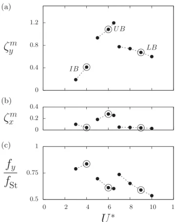
In the present study, which is part of a Ph.D. work [32], the spanwise patterns emerging in the flow past a fixed or freely vibrating circular cylinder are analyzed, on the basis of numerical simulation results, at Re = 3900; this value of Re was often selected in prior works as a typical case of the early turbulent regime [33]. The spanwise patterns developing once the cylinder oscillates are investigated in conditions naturally arising for a bluff body free to move in the current, by considering cases of vortex-induced vibrations (VIVs). The principal flow-structure interaction aspects of the problem have been examined in a previous work [34] and comparable systems have been studied by Jauvtis and Williamson [35], Dahl et al. [36], Navrose and Mittal [37], and Cagney and Balabani [38]. Figure2

shows the evolution of the body responses as a function of the reduced velocity U∗_{, defined as the}

inverse of the nondimensional natural frequency of the oscillator. The amplitudes and frequencies are nondimensionalized by the body diameter and current velocity. Large-amplitude oscillations [Figs.2(a)and2(b)] are reached over a well-defined range of reduced velocities, called the lock-in range, where the dominant frequency of wake unsteadiness and body oscillation frequency coincide [39–42]. Three response branches can be identified, the initial (IB), upper (UB), and lower (LB) branches, as indicated in the figure. The frequency ratio between the in-line and crossflow oscillations is equal to 2 over the lock-in range. The evolution of the crossflow oscillation frequency fy,

normal-ized by the wake frequency in the fixed body case (Strouhal frequency fSt), is plotted in Fig.2(c). In

the present work, the flow behavior is studied over the lock-in range for three values of the reduced velocity U∗_{∈ {3,6,9}, i.e., one typical case in each branch. As shown in Fig.2, these cases cover wide}

ranges of oscillation amplitudes and frequencies. The dominant features of the three-dimensional flow structures are explored in both the shear layer and wake regions. The spanwise patterns are characterized in terms of amplitudes and spatial wavelengths, with particular attention paid to their streamwise evolution within each region and to their possible alteration once the cylinder oscillates. The methodology employed in this study is described in Sec.II. A qualitative overview of the flow is presented in Sec.III. The spanwise patterns are quantitatively examined in Sec.IV. Some elements of physical analysis are discussed in Sec.V. The principal findings of this work are summarized in Sec.VI.

St

FIG. 2. Structural responses of an elastically mounted circular cylinder subjected to vortex-induced vibrations at Re = 3900: (a) in-line and (b) crossflow oscillation amplitudes (nondimensionalized by the cylinder diameter) and (c) crossflow oscillation frequency normalized by the Strouhal frequency (vortex shedding frequency in the fixed body case), as functions of the reduced velocity. Circles indicate the three typical cases examined in the present work, in addition to the fixed body case.

II. METHOD

The physical system and the numerical method are presented in Sec.II A. The data processing approach is described in Sec.II B.

A. Physical system and numerical method

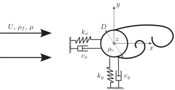
The physical system is analogous to that described by Gsell et al. [34]. A sketch of the physical configuration is presented in Fig.3. A circular cylinder of diameter D is immersed in a crossflow. The body axis (z axis) is located at (x,y) = (0,0) in quiescent fluid. The current is parallel to the x axis and characterized by its velocity U, density ρf, and dynamic viscosity µ. All the physical

quantities are made nondimensional by D, U, and ρf. The Reynolds number based on U and D, Re =

ρfU D/µ, is set to 3900. The flow dynamics is governed by the three-dimensional incompressible

Navier-Stokes equations. In the elastically mounted body case, the cylinder is free to oscillate in the in-line (x-axis) and crossflow (y-axis) directions. The oscillator is characterized by the body mass per unit length ρcand structural stiffnesses kxand kyand dampings cxand cy, in both directions. The

cylinder nondimensional displacement, velocity, and acceleration in the in-line (crossflow) direction are denoted by ζx, ˙ζx, and ¨ζx(ζy, ˙ζy, and ¨ζy), respectively. The body dynamics is governed by a forced

FIG. 3. Sketch of the physical configuration.

structural stiffnesses are the same in both directions (kx = ky= k). The nondimensional body mass

is defined as m = ρc/ρfD2; it is set to 2. The nondimensional natural frequency of the oscillator

f_{nat= D/2πU}√k/ρcis used to define the reduced velocity U∗= 1/fnat. Three values, typical of

each branch of VIV response, are considered here, U∗_{∈ {3,6,9}.}

The behavior of the coupled flow-structure system is predicted by direct numerical simulation of the three-dimensional Navier-Stokes equations. The computations are performed with the finite-volume code Numeca Fine/Open [43]. The term direct numerical simulation is used to indicate that no additional modeling is employed before numerical integration of the Navier-Stokes equations. It should however be mentioned that the spatial and temporal resolutions of the computations, as well as the numerical dissipation terms employed in the discretization schemes, limit the scales that can be simulated. Details of the numerical method, as well as convergence and validation results, have been reported in a previous paper [34]. Additional information concerning the computational domain and spatial and temporal discretizations is given in AppendixA. A comparison of the present results with prior works, in the fixed body case, is provided in AppendixB.

B. Data processing

The three dimensionality of the flow is analyzed along spanwise lines. Two types of lines are considered: L1, located in the separated shear layers, and L2, further in the wake. A schematic view

of the locations of L1 and L2 is presented in Fig. 4. The frame attached to the cylinder axis, in

translation with respect to the fixed (x,y,z) frame, is denoted by (xc,yc,z). A tracking method is

used to capture the instantaneous position of the shear layers. A similar method was employed by Rai [21] and is extended here to the case of oscillating bodies. The method involves a new frame

(η,ξ,z). This frame is attached to the axis of the body and the η axis (ξ axis) is parallel (normal) to the instantaneous oncoming flow velocity Vin, defined as Vin= [Vin,x,Vin,y,0] = [1 − ˙ζx, − ˙ζy,0] in the

(x,y,z) frame. A separated shear layer is defined, in the near region, as an isosurface Vη= 0.75|Vin|,

where Vη is the η component of the flow velocity field. A line L1 is defined as a line located at a

given distance η from the cylinder, in the above-defined isosurface. Lines L1 in the upper (ξ > 0)

and lower (ξ < 0) shear layers are denoted by L+

1 and L−1. Lines L2 are fixed in the laboratory

frame (x,y,z). Their crossflow position is set to match the region of minimum (maximum) span-and time-averaged spanwise vorticity, i.e., the region crossed by clockwise (counterclockwise) wake vortices. Upper (y > 0) and lower (y < 0) lines are denoted by L+

2 and L−2, respectively. When the

positive and negative wake vortices are aligned, the crossflow position of L2is set to zero.

The flow quantities measured along lines L1 and L2 are averaged over selected time series. A

phase average is used on lines L1. As shown in the following, this approach ensures that the data

are collected on well-developed shear layers and thus a consistent comparison between the different oscillating body cases. The phase is based on the crossflow displacement of the body. The symmetry of the system is taken into account when computing the phase-averaged value: The shear layer at phase φ is expected to be symmetric with the opposite shear layer at phase φ + π. The phase-averaged value of a quantity 9, at streamwise distance η and phase φ, is defined as

h9ip,L1(η,φ) = 1₂[h9ip,L+1(η,φ) + h9ip,L−1(η,φ + π)], (1) where h ip,L+1 and h ip,L−1 denote the phase-averaged values on lines L

+

1 and L−1, which are obtained

over three oscillation cycles. For each cycle, five snapshots close to the selected phase are considered for averaging. In the fixed body case, the above phase average is replaced by a time average, denoted by h it,L1 and similar to that used on lines L2. On lines L2, in the wake region, time averaging is preferred to the above phase-averaging procedure for a more rigorous comparison with prior experimental results. However, it should be mentioned that the general trends identified in this region based on time-averaged flow quantities have been confirmed by employing the same phase-averaging procedure as in the shear layer region: The contrasted behaviors observed in the shear layer and wake regions do not depend on the nature (time or phase) of the averaging procedure. Due to the system symmetry, the time-averaging operator applied on lines L2 involves both L+2 and L−2. The

time-averaged value of a quantity 9, at streamwise distance x, is defined as h9it,L2(x) = 1₂[h9it,L+

2(x) + h9it,L−2(x)], (2)

where h it,L+

2 and h it,L−2 denote the time-averaged values on lines L

+

2 and L−2.

The distribution of the crossflow component of the vorticity, along lines L1 and L2, is used to

quantify the spanwise patterns of the flow. The crossflow component of the vorticity was selected as it provides a clear visualization of the three-dimensional flow structure, as shown in the following. It has been verified that the quantitative observations reported here, especially regarding the evolution of the spanwise wavelength of the flow, do not depend on the vorticity component considered in the analysis. In the shear layer region (lines L1), the vorticity component aligned with the ξ axis

of the mobile frame (ωξ) is considered, while the vorticity component aligned with the fixed y axis

(ωy) is considered in the wake region (lines L2). It is recalled that in the fixed body case, η = x and

ωξ = ωy.

The amplitudes of the spanwise fluctuations along lines L1and L2, denoted by Az1and Az2, are

defined as

Az1(x) = hω′yit,L1(x) (fixed body), (3a)

Az1(η,φ) = hω′ξip,L1(η,φ) (oscillating body), (3b)

Az2(x) = hω′yit,L2(x) (all cases), (3c)

where the prime designates the root-mean-square value in the spanwise direction. The Hilbert transform is used to compute the local spanwise wavelength of vorticity fluctuations. Considering a

vorticity signal ω(z), the analytic signal is defined as ωa_{(z) = ω(z) + iH}

ω(z), where Hωis the Hilbert

transform of ω. In exponential form, the analytic signal can be written ωa_{(z) = Ä(z)e}iϕ(z)_{, where Ä}

and ϕ are the local amplitude and local phase of ω. The local (z-dependent) spanwise wavelength is defined as λl

z= 2π/(dϕ/dz). The probability density function (PDF) of λlzalong the body length is

denoted by P(λl

z). The PDF is used to determine the typical instantaneous wavelength λiz= P(λlz),

where the overline denotes the average of the 10% most frequent wavelengths in the PDF. The typical instantaneous wavelengths of ωξand ωyare computed on lines L1and L2, respectively. The averaged

spanwise wavelengths in the shear layer and wake regions, denoted by λz1and λz2, are then defined as

λz1(x) =­λiz

®

t,L1(x) (fixed body), (4a)

λz1(η,φ) =­λiz ® p,L1(η,φ) (oscillating body), (4b) λz2(x) =­λiz ®∗ t,L2(x) (all cases). (4c)

In (4c), a selective time averaging (denoted by the asterisk superscript) is performed, by only considering the samples where a clear dominant wavelength appears in the PDF, i.e., where the cumulative probability of the 10% most frequent wavelengths is larger than a given value, set to 0.45 in the following. The time variability of the spanwise wavelength about its averaged value is quantified, in each region, by the standard deviations

eλz1(x) =q­¡λiz− λz1

¢2®

t,L1(x) (fixed body), (5a)

eλz1(η,φ) =q­¡λiz− λz1 ¢2® p,L1(η,φ) (oscillating body), (5b) eλz2(x) =q­¡λiz− λz2 ¢2®∗ t,L2(x) (all cases). (5c)

III. OVERVIEW OF THE FLOW

The flow patterns observed in the (x,y) plane are depicted in Fig.5, which represents instantaneous isocontours of the span-averaged spanwise vorticity (ωz) in the fixed and oscillating body cases. The

spanwise lines L+

2 (defined in Sec.II B), used in the following to analyze the spanwise patterns

in the wake region, are indicated by red dots in the plots. In the fixed body case [Fig. 5(a)], the wake exhibits a typical von Kármán vortex street pattern. The formation of the large-scale spanwise vortices occurs close to x = 2, as also reported in prior works [44]. Upstream, well-defined shear layers, separating from the body, can be noted. The (x,y) flow pattern is modified when the body oscillates [Figs.5(b)–5(d)], as previously discussed by Gsell et al. [34], on the basis of span- and phase-averaged visualizations. Following the terminology of Williamson and Roshko [3], a 2S pattern is identified for U∗_{= 3 and U}∗_{= 6, while a 2P pattern is noted for U}∗_{= 9. Significant variations of}

the length scales of the flow pattern are also observed. For example, the typical streamwise distance between the spanwise vortical structures for U∗ _{= 9 is roughly twice as large as in the fixed body case.}

The crossflow width of the wake also varies from one case to the other. The alteration of the flow length scales in the (x,y) plane is further discussed in Sec.V. Vortex formation tends to occur closer to the body when it vibrates, which corroborates prior visualizations of flows past oscillating cylinders [45]. The three dimensionality of the flow can be illustrated by the magnitude of the streamwise (ωx)

and/or crossflow (ωy) vorticity components. The projection of the vorticity vector on the (x,y) plane is

referred to as planar vorticity and is denoted by ωp. The patterns of ωpin the (x,y) plane are examined in Fig.6, which shows instantaneous isocontours of the span-averaged, planar vorticity magnitude |ωp| =√ω2_{x+ ω}2_yin the four cases studied. In the fixed body case [Fig.6(a)], the planar vorticity is concentrated close to the large-scale spanwise vortices [Fig.5(a)], but also in the regions connecting these vortices; the high level of planar vorticity in these regions is consistent with the mechanism of vorticity stretching between wake vortices, described in prior works [4,6]. The behavior of the planar

FIG. 5. Flow patterns in the (x,y) plane: instantaneous isocontours of the span-averaged, spanwise vorticity (ωz_{∈ [−2,2]) in the (a) fixed and (b)–(d) oscillating body cases, for (b) U}∗_{= 3, (c) U}∗_{= 6, and (d) U}∗_{= 9.} In each case, red dots indicate the positions of lines L+

2 (defined in Sec.II B). In (b)–(d), ζy = 0 and the body is moving downward.

vorticity is globally analogous when the body oscillates [Figs.6(b)–6(d)]. In all cases studied, the region of maximum planar vorticity is located close to the body. However, it appears that the planar vorticity magnitude in the region of the detached shear layers is substantially lower in the fixed body case than in the oscillating body cases.

The flow patterns emerging in the third (z) direction are examined in the following. A global visualization of the three-dimensional flow is presented in Fig. 7. In the four cases studied, an instantaneous isosurface of the Q criterion [31] is colored by isocontours of the crossflow vorticity (ωy). The Q criterion highlights a number of small elongated vortices, mainly aligned in the (x,y)

plane. Their locations coincide with the regions of large planar vorticity magnitude depicted in Fig.6. These vortices have often been described as streamwise vortices in prior studies. However, due to their alignment in the (x,y) plane and their oblique orientation in this plane, the term planar vortices is preferred in the following to designate these flow structures. The planar vortices are observed in both the fixed and oscillating body cases. While body motion is generally expected to decrease the three dimensionality of the flow, the density of planar vortices in the wake region and their magnitude do not significantly vary from one case to the other. In this region, the planar vortices tend to be more regularly aligned in the (x,y) plane when the body oscillates. This suggests that body motion may be associated with a homogenization of the three-dimensional patterns. The planar vortices are generally observed over the entire body length. They define a typical spanwise length scale of the flow structure. Localized regions without planar vortices may however be encountered [U∗_{= 9,}

FIG. 6. Flow patterns in the (x,y) plane: instantaneous isocontours of the span-averaged, planar vorticity magnitude (|ωp| ∈ [0,2]) in the (a) fixed and (b)–(d) oscillating body cases, for (b) U∗= 3, (c) U∗= 6, and

(d) U∗_{= 9. In (b)–(d), ζ}

y = 0 and the body is moving downward.

A closer view of the three-dimensional flow in the shear layer region is presented in Fig.8. A higher value of the Q criterion is used in comparison with Fig.7 to highlight the dominant flow features encountered close to the body. In order to connect the three-dimensional patterns with the flow in the (x,y) plane, slices of the domain at z = 0, colored by isocontours of the spanwise vorticity, are also shown in each case. In the fixed body case [Fig.8(a)], elongated planar vortices appear in the region of formation of the large-scale spanwise vortices. Upstream, in the shear layer region, no vortices are noted. More planar vortices seem to develop in the oscillating body cases (the Q-criterion level is kept constant in all cases). For U∗ _{= 3 [Fig.8(b)], planar vortices can be identified between}

the cylinder and the forming spanwise vortex. The enhancement of planar vortex formation in the shear layer region, when the body vibrates, is confirmed by the visualizations reported for U∗_{= 6}

and U∗ _{= 9 [Figs.8(c)and8(d)]. Such enhancement is consistent with the increased planar vorticity}

magnitude noted close to the cylinder when it oscillates (Fig.6).

In the near region, particular attention is paid to the three-dimensional structure of the shear layers separating from the cylinder; the tracking method employed to capture the shear layers is described in Sec.II B. An example of shear layer tracking is presented in Fig.9, for U∗_{= 6, i.e., in}

the case of maximum oscillation amplitudes. In Figs.9(a),9(c), and9(e), the evolution of the shear layers as the body oscillates is visualized by plotting isocontours of the span-averaged spanwise vorticity at three instants of an oscillation cycle. Large deformations of the shear layers can be noted in the (x,y) plane. In this example, where the body is moving downward, a well-defined upper shear layer (blue) can be identified. In contrast, the lower shear layer (orange) is very short and does not clearly separate from the body. The span-averaged location of the surface captured by

(a)

(c) (d)

(b)

FIG. 7. Global visualization of the three-dimensional flow: instantaneous isosurface of the Q criterion (Q = 0.1) colored by isocontours of the crossflow vorticity (ωy ∈ [−1,1]) in the (a) fixed and (b)–(d) oscillating body cases, for (b) U∗_{= 3, (c) U}∗_{= 6, and (d) U}∗_{= 9. In (b)–(d), ζ}

y = 0 and the body is moving downward.

the tracking method is indicated by red dots in Figs.9(a),9(c), and9(e); it matches the location of the shear layer visualized via spanwise vorticity isocontours. The corresponding three-dimensional surface, colored by isocontours of surface elevation (along the ξ axis), is shown at each instant in Figs.9(b),9(d), and9(f). In Fig.9(b), a short shear layer detaches from the body. As the body moves downward [Figs.9(d)and9(f)], the shear layer develops: Its length increases and a spanwise wake vortex forms. This development is accompanied by a pronounced three-dimensional deformation of the shear layer.

A visualization of the three-dimensional shear layer separating from the upper side of the body (captured by the above-mentioned method) is presented in Fig.10, in the four cases studied. In the oscillating body cases, the snapshots are shown for ζy= 0 and the body moving downward, i.e.,

the phase at which a well-developed shear layer has been observed for U∗_{= 6 (Fig.9). In the fixed}

body case, the crossflow vorticity, which is used to color the shear layer surface, exhibits spanwise patterns similar to those reported by Rai [21], at the same Reynolds number. A deformation of the shear layer, which coincides with the patterns of vorticity, can also be noted along the entire span. Similar features are observed when the cylinder moves; however, the amplitudes of crossflow vorticity (ξ -axis component) fluctuations and shear layer deformations tend to increase in the oscillating body cases. The spanwise wavelength that emerges in the shear layer seems to be altered when the body oscillates and to vary from one moving body case to the other. These aspects will be examined quantitatively in Sec.IV.

In order to shed light on the dominant spanwise patterns, flow quantities are collected along spanwise lines placed downstream of the body. Two types of lines are considered, as described

FIG. 8. Visualization of the three-dimensional flow close to the body: instantaneous isocontours of the spanwise vorticity (ωz_{∈ [−10,10]) in the plane z = 0 and isosurface of the Q criterion (Q = 10) colored by} isocontours of the crossflow vorticity (ωy_{∈ [−1,1]) in the (a) fixed and (b)–(d) oscillating body cases, for (b)} U∗_{= 3, (c) U}∗_{= 6, and (d) U}∗_{= 9.}

FIG. 9. Visualization of the shear layers separating from the body, for U∗_{= 6: (a), (c), and (e) isocontours} of the span-averaged, spanwise vorticity (ωz_{∈ [−2,2]) and (b), (d), and (f) three-dimensional upper shear layer} colored by isocontours of surface elevation (ξ ∈ [0.6,1.2]), at three instants during an oscillation cycle. In (a), (c), and (e), the trajectory, position, and velocity of the body are shown and red dots indicate the span-averaged location of the surface captured by the shear layer tracking method (described in Sec.II B).

in Sec. II B: lines L1, located in the shear layers [moving frame (η,ξ,z)], and lines L2, placed

further in the wake, in zones crossed by the large-scale spanwise vortices [laboratory frame (x,y,z)]. Selected time series of the crossflow vorticity along lines L+

1(η = 1) and L+2(x = 5) are shown in

Fig.11, for the four cases studied. As mentioned in Sec.II B, the term crossflow vorticity is used to designate the vorticity component aligned with the ξ axis of the mobile frame in the shear layer region (lines L1) and the component aligned with the fixed y axis in the wake region (lines L2). The

crossflow vorticity in the shear layer separating from the fixed body is depicted in Fig.11(a). The selected time series last approximately four vortex shedding periods. At any instant, the vorticity exhibits spanwise fluctuations over the entire body, with a relatively-well-defined wavelength. The spatiotemporal structure of the flow is essentially perpendicular to the body axis, as expected from the spatial distribution of the crossflow vorticity in Fig.10(a). Distinct patterns, characterized by rapid

FIG. 10. Three-dimensional shear layer separating from the body: upper shear layer colored by instantaneous isocontours of the crossflow vorticity (ωξ_{∈ [−1,1]) in the (a) fixed and (b)–(d) oscillating body cases, for (b)} U∗_{= 3, (c) U}∗_{= 6, and (d) U}∗_{= 9. In the oscillating body cases, ζ}

y= 0 and the body is moving downward.

temporal fluctuations of the vorticity in localized regions of the span, are also noted in Fig.11(a); an instance of this phenomenon is indicated by a black rectangle in the figure. These localized events, also reported by Rai [21], relate to the presence of shear layer vortices, called transition waves by Bloor [11]. A brief spectral analysis of the vorticity fluctuations associated with the shear layer vortices is presented in AppendixC.

The behavior of the crossflow vorticity in the shear layer, when the body oscillates, is depicted in Figs.11(c),11(e), and11(g), for U∗ _{∈ {3,6,9}. Since the shear layer may be substantially deformed}

or shortened once the body moves, an additional criterion is employed to confirm that lines L1

are located in high-vorticity regions: Some samples are discarded, based on the magnitude of the spanwise vorticity ωz, averaged along the considered spanwise line; below a given level, the line is

not representative of a shear layer. Discarded samples are indicated by striped areas in Figs.11(c)

and11(e). Large spanwise fluctuations of ωξ can be noted in the three oscillating body cases. As

in the fixed body case, a typical spanwise length scale (apparently lower than in the fixed body case) emerges and the dominant spatiotemporal structure of the flow is mainly perpendicular to the body axis. It should be mentioned that the range of vorticity values considered in the oscillating body cases is substantially wider than in the fixed body case (ωξ ∈ [−10,10] versus ωξ ∈ [−2,2]),

which confirms the amplification of the spanwise fluctuations observed in Fig.10. Some shear layer vortices, comparable to those observed in the fixed body case, are also noted for U∗ _{= 9, although}

less clearly defined. Such vortices cannot be identified for U∗_{= 3 and U}∗_{= 6, which may be due}

to the short lifetime of the detached shear layers.

The time series of the crossflow vorticity in the wake region [line L+

2(x = 5)] are presented in

Figs. 11(b),11(d),11(f), and 11(h). It is recalled that the crossflow position of L+

2 varies from

one case to the other (Fig.5). In each case, ωy exhibits spanwise fluctuations, with a typical spatial

wavelength which seems larger than that observed in the shear layer region. The spanwise fluctuations are coupled with a time-periodic amplitude modulation, at the spanwise vortex shedding frequency.

FIG. 11. Time series of the spanwise patterns in the shear layer and wake regions: (a), (c), (e), and (g) ωξ on line L+

1(η = 1) and (b), (d), (f), and (h) ωyon line L+2(x = 5), in the (a) and (b) fixed and (c)–(h) oscillating body cases, for (c) and (d) U∗_{= 3, (e) and (f) U}∗_{= 6, and (g) and (h) U}∗_{= 9. The isocontours are distributed} in ranges (a) ωξ_{∈ [−2,2], (c), (e), and (g) ω}ξ∈ [−10,10], and (b), (d), (f), and (h) ωy∈ [−2,2]. In (a), a black rectangle indicates an instance of shear layer vortices. In (c) and (e), striped areas denote discarded samples (low-vorticity level).

This modulation is expected due to the inhomogeneous distribution of flow three dimensionality in the (x,y) plane: As previously shown in Fig.6, it concentrates in the spanwise vortices and in regions connecting the spanwise vortices. Contrary to what was observed in the shear layers, the magnitudes and wavelengths of vorticity fluctuations in the wake region are globally comparable in the fixed and oscillating body cases.

To summarize, these qualitative observations of the flow emphasize its three dimensionality which is characterized, in both fixed and oscillating body cases, by pronounced fluctuations distributed along the span. Two dominant features have been highlighted: the spanwise undulations of the shear layers separating from the body and the development of elongated planar vortices. This first overview suggests that flow three dimensionality could be altered differently in the shear layer and wake regions, once the body oscillates. In order to provide a more quantitative vision of the three-dimensional structure of the flow and confirm the above observations, a systematic analysis of the flow spanwise fluctuations is presented in the next section.

IV. QUANTITATIVE ANALYSIS OF THE SPANWISE PATTERNS

The spanwise patterns observed qualitatively in Sec. IIIare quantified through the amplitudes Az1 and Az2 (Sec.IV A) and wavelengths λz1 and λz2(Sec. IV B) of the spanwise fluctuations of

the crossflow vorticity component. These quantities and associated averaging procedures are defined in Sec. II B. In the shear layer region, the time series of vorticity collected along lines L1 are

discontinuous in some cases (Fig.11). In the oscillating body cases, a phase-averaging procedure is employed in this region. In this section, the analysis is performed for {ζy = 0, ˙ζy<0}; this phase is

selected for comparison since a well-developed shear layer is observed at this point of the oscillation cycle in all cases studied (Fig.10). The influence of the selected phase on the results will be discussed in Sec.V. In the fixed body case, the phase averaging is replaced by a time averaging. For all cases, in the wake region (lines L2), time-averaged data are examined.

A. Amplitude of spanwise fluctuations

The streamwise evolution of Az1 and Az2 is presented in Fig. 12. In the fixed body case, a

continuous increase of the spanwise fluctuation amplitude, as a function of the streamwise distance, is

FIG. 12. Streamwise evolution of the spanwise fluctuation amplitude, in the fixed and oscillating body cases. In the oscillating body cases, the amplitudes Az1are determined for {ζy= 0, ˙ζy <0} (Sec.II B).

observed in the shear layer region. The amplitude keeps increasing at the beginning of the wake region and a maximum value is reached close to x = 3, i.e., near the region of formation of the spanwise wake vortices. This corroborates the qualitative observations based on Fig.6(a). The evolution of Az1 and Az2 in the oscillating body cases is also plotted in Fig.12. For U∗ = 3 and U∗= 9, the

range of η is limited to η ∈ [0,1] since the shear layer does not extend further downstream. When the cylinder oscillates, the amplitude of the spanwise fluctuations is dramatically altered in the shear layer region; it is generally larger in this case, as expected from the visualizations reported in Figs.8

and10. For example, the peak amplitude in this region for U∗_{= 6 is roughly 6 times larger than in}

the fixed body case. The streamwise trend of Az1is comparable in the three oscillating body cases:

a steep increase in the very near region (close to the area of spanwise vortex formation), followed by a much lower increase or a decrease. Some slight differences can be noted in the wake region for x ∈ [2,4]. Further downstream (x > 4), the relatively constant amplitudes are close in all cases studied, including in the fixed body case. The global upstream shift of the peak amplitude in the oscillating body cases, compared to the fixed body case, may be connected to the upstream shift of the spanwise vortex formation region, previously observed in Fig.5. The evolution of Az1and Az2

suggests that the alteration of the spanwise fluctuations, associated with body motion, is essentially localized close to the cylinder, in the shear layer region.

B. Wavelength of spanwise fluctuations

The local wavelength of the spanwise pattern (λl

z) is determined via the Hilbert transform, as

described in Sec.II B. At each instant, the PDFs of λl

zare computed along lines L1and L2. In order

to illustrate the postprocessing applied to the simulation data, the time series of the PDFs obtained along L+

1(η = 1) and L+2(x = 5) are plotted in Fig.13, in the four cases studied. In the shear layer

region [Figs.13(a),13(c),13(e), and13(g)], the PDFs are sharp and a dominant wavelength, referred to as typical instantaneous wavelength λi

z(defined in Sec.II B) clearly emerges; in each case, this

dominant wavelength is close to constant as a function of time. In the wake region [Figs.13(b),13(d),

13(f), and13(h)] the PDFs present broader distributions and a criterion, described in Sec.II B, is employed to select the time instants at which a dominant wavelength can be identified. These time instants are indicated by gray dots in the plots. In each case, the typical instantaneous wavelength exhibits more time variability than in the shear layer region, but its deviation from the time-averaged value is still limited.

The evolution of the averaged spanwise wavelength, λz1in the shear layer region and λz2in the

wake region, as a function of the streamwise distance, in the fixed body case, is depicted in Fig.14. The wavelength exhibits a continuous streamwise evolution. Distinct trends can be observed in the shear layer and wake regions: The wavelength decreases as a function of the streamwise distance in the shear layer region, while it tends to increase with x further downstream. A minimum wavelength close to 0.5 diameters is noted around x = 2. The time variability of the wavelength is quantified by its standard deviation [eλz1 and eλz2, defined by (5)]; the values of λz1±eλz1 and λz2±eλz2 are

indicated by error bars in the figure. The time variability of the wavelength remains small compared to its streamwise variation.

The experimental results of Mansy et al. [5] and Chyu and Rockwell [9] are also plotted in Fig.14. The data of Mansy et al. [5] are presented for two crossflow positions; the wavelengths reported by Chyu and Rockwell [9] are averaged in the crossflow direction. The wavelength jump observed by Chyu and Rockwell [9] at x ≈ 1 is similar to that reported by Mansy et al. [5] at x ≈ 2 and y = 1. This jump occurs close to the region of formation of the spanwise wake vortices. The difference of Re between these studies (Re = 600 versus Re = 104_{) leads to distinct vortex formation lengths [44],}

which can explain the shift observed in the streamwise location of the wavelength jump. The data of Mansy et al. [5] show a different trend at y = 0.5, where no jump appears in the range of streamwise distances investigated, as in the present results. This highlights the substantial impact of the crossflow location of the sampling point on the measured wavelength close to the body. In the present work, the wavelength is determined in the shear layers. In the fixed body case, the upper shear layer is located

FIG. 13. Time series of the PDF of the local spanwise wavelength in the shear layer and wake regions: (a), (c), (e), and (g) on line L+

1(η = 1) and (b), (d), (f), and (h) on line L+2(x = 5), in the (a) and (b) fixed and (c)–(h) oscillating body cases, for (c) and (d) U∗_{= 3, (e) and (f) U}∗_{= 6, and (g) and (h) U}∗_{= 9. The isocontours of} the PDF are distributed in the range [0,2]. In (b), (d), (f), and (h), gray dots indicate the samples considered in the selective time-averaging procedure (h i∗

t,L2, defined in Sec.II B). In (c) and (e), striped areas denote discarded

Ref. [5], Ref. [5],

Ref. [9] Present work Present work,

FIG. 14. Streamwise evolution of the spanwise wavelength in the fixed body case: comparison between the present results and the experimental measurements of Mansy et al. [5] (Re = 600) and Chyu and Rockwell [9] (Re = 104_{). For the present results, error bars indicate the standard deviation of the wavelength around the} averaged value [defined by (5)]. The wavelengths obtained at y = 1 are also plotted for comparison.

close to y = 0.5 [Fig.5(a)]. In order to visualize the influence of the sampling point location, the wavelengths obtained at y = 1, on the basis of the present simulation results, are reported in Fig.14. At y = 1, a rapid change of the wavelength, qualitatively comparable to that observed in prior studies, can be noted at x ≈ 3. For x > 3, the wavelengths are close to those obtained along lines L2: There

is no major effect of the sampling point location in this zone; this is also suggested by the results of Mansy et al. [5]. In the near region (x < 3), the wavelengths are significantly lower than those previously determined in the shear layer, which confirms the impact of the sampling point location close to the body. Direct comparison with previous works may thus be questionable in this region. It should be mentioned that the amplitude of the spanwise fluctuations almost vanishes around y = 1 (Az1≈ 0); the quantification of the wavelength in this zone may therefore be less relevant than in the

shear layer, i.e., the area studied in the present work. The general evolution of λz2further in the wake

(x > 3) is comparable to that reported by Mansy et al. [5], but the wavelengths are lower is the present study. In this part of the wake region where the sampling point location has a limited influence, this trend may denote an effect of the Reynolds number on the spanwise wavelength (Re = 600 in the experiments of Mansy et al. [5] versus Re = 3900 in the present simulations).

The streamwise evolutions of the spanwise wavelength in the fixed and oscillating body cases are compared in Fig.15. The overall trend of the wavelength is similar in all cases studied. The alteration of the wavelength associated with body motion is concentrated in the shear layer region. In this region, lower minimum values of λz1, still close to 0.5D, can be reached once the cylinder

oscillates. In contrast, there is no important modification of λz2in the wake region; the variation of

the wavelength between the different cases is generally smaller than its time variability for a given case (indicated by the error bars for U∗_{= 3, which is the case of maximum variability). In addition,}

the variation of λz2in this region is negligible compared to the variation of the (x,y) typical length

scales of the wake, as discussed in Sec.V.

The above results concerning the spanwise wavelength reveal globally comparable streamwise evolutions in all cases, with decreasing and increasing trends in the shear layer and wake regions, respectively. They also confirm that the spanwise structure of the flow is differently altered in each region, once the cylinder vibrates: In the shear layer region, the amplification of the spanwise fluctuation magnitude noted in Sec. IV A is accompanied by a clear reduction of the spatial wavelength, while the spanwise pattern is essentially unaltered in the wake region.

FIG. 15. Streamwise evolution of the spanwise wavelength, in the fixed and oscillating body cases. In the oscillating body cases, the wavelengths λz1are determined for {ζy = 0, ˙ζy<0} (Sec.II B). Error bars indicate the standard deviation of the wavelength around the averaged value [defined by (5)] for U∗_{= 3, i.e., the case} of maximum variability.

V. DISCUSSION

Some additional elements are examined in this section, which aims at connecting the present results with prior works and at providing some complementary analysis of the flow structure. The discussion is articulated around five principal points.

(i) Mechanism of spanwise fluctuation amplification.In order to explain the formation of planar

vortices downstream of the body, Wu et al. [6] employed a concept of vortex filament. In this model, a vortex line, initially aligned with the z axis, exhibits a localized kink in response to any flow disturbance. When approaching a high-strain region, between two primary spanwise wake vortices, the distorted vortex line is stretched, resulting in an increase of the vorticity magnitude and in the formation of planar vortices. A comparable model had been proposed by Wei and Smith [13] in the shear layer region: A distorted vortex line in the shear layer is stretched as it approaches the forming spanwise wake vortex. An amplification of planar vorticity may thus be expected in the region of formation of the spanwise wake vortices. The present results tend to corroborate this model: A streamwise increase of the spanwise pattern amplitude is indeed observed close to the body (Fig.12) and the peak amplitude is found in the region of formation of the spanwise vortices (Fig.5). In the oscillating body cases, a substantial amplification of the spanwise fluctuations has been noted in the shear layers. On the basis of the above model, a possible mechanism at the origin of this amplification could be the additional stretching induced by body motion. This mechanism would mainly impact the flow close to the body, which is consistent with the present results.

(ii) Transient behavior of the shear layers.A schematic view of the boundary layer separating

from the body is presented in Fig.16. The nondimensional local momentum thickness at separation can be quantified as follows, at each spanwise location and each time instant:

δ_sl ₌ Z nm 0 Vt Vm µ 1 − Vt Vm ¶ dn, (6)

where n is the distance normal to the wall at the separation point, Vt the tangential flow velocity

component [in the (x,y) plane], and Vmthe maximum value of Vtin the boundary layer, reached at a

FIG. 16. Schematic view of the boundary layer separating from the cylinder.

body) value of δl

s is denoted by δsand referred to as momentum thickness in the following. Typical

values of δsin the present cases range from 0.004 to 0.006. In plane mixing layers, the flow generally

exhibits a transient regime before reaching a self-similar behavior associated with a linear growth of the shear layer thickness as a function of the streamwise distance [46]. The streamwise extent of the transient regime is of the order of a few hundred times the initial momentum thickness. Considering δsas an equivalent initial momentum thickness, the transient regime of the shear layers separating

from the cylinder is thus expected to extend over a few body diameters (it is recalled that δs is

normalized by the body diameter). Therefore, the separated shear layers observed downstream of the body are in a transient regime. For plane mixing layers, the transient regime is accompanied by significant variations of the amplitude and wavelength of the spanwise pattern [27,28]: In particular, the early development of the mixing layer is characterized by a decrease of the spanwise wavelength. Such behavior is also noted in the present simulation results (Fig.15), which further highlights the analogy between plane mixing layers and the shear layers separating from the cylinder.

(iii) Scaling of λz1with δsand effect of the instantaneous Reynolds number.The analogy with plane

mixing layers raises the question of the connection between the typical length scales of the cylinder shear layers and the momentum thickness at separation. This aspect is examined in Fig.17(a), which

Ref. [47] Ref. [48] Ref. [49]

FIG. 17. Scaling of the shear layer spanwise wavelength with the momentum thickness of the boundary layer at separation: (a) streamwise evolution of λz1normalized by δs and (b) evolution of δs as a function of the Reynolds number (Re in the fixed body case and Reipin the oscillating body cases). In the oscillating body cases, the phase-averaged values are determined for {ζy= 0, ˙ζy<0} in (a) and different phases are considered in (b). In (a), a dash-dotted line (λz1/δs_{= 90) indicates the typical value of the normalized wavelength in} the plateau region; an error bar shows the typical variation (standard deviation) of λz1/δsaround this plateau value at different phases, for U∗_{= 3 and η/δs≈ 150. In (b), the momentum thickness values issued from the} experimental studies of Thom [47], Green [48], and Fage [49] are also reported for comparison.

represents the streamwise evolution of the spanwise wavelength normalized by δs in the four cases

studied; the streamwise distance is also normalized by δs. In the oscillating body cases, δsand λz1are

determined for {ζy= 0, ˙ζy <0}, i.e., the same phase as in Sec.IV. As previously observed, all cases

exhibit an initial decrease of the wavelength in the region very close to the cylinder. The streamwise extent of this decreasing trend varies from one case to the other, even after normalization of η by δs. Further downstream, the normalized wavelengths tend to collapse in a plateau region, where

λ_z1/δs≈ 90, in all cases studied. This relatively constant value of λz1/δs persists at other phases

of body displacement; this is illustrated by the error bar in Fig.17(a), which indicates the typical variation (standard deviation) of λz1/δsin the plateau region when changing the value of the phase,

for U∗_{= 3. The present results suggest that the spanwise wavelength in the plateau region scales}

with the momentum thickness of the boundary layer at separation, the latter being altered when the body moves, as shown in the following. This scaling is comparable to that observed with the initial momentum thickness in plane mixing layers; it corroborates the above-mentioned connections between both flow configurations.

In the fixed body case, the boundary layer thickness varies as a function of the Reynolds number. The value of δs obtained from the present simulation data is plotted in Fig.17(b)and compared to

the momentum thickness values reported by Prasad and Williamson [16], which were issued from prior experimental studies at higher Re [47–49]. A global decrease is observed as a function of the Reynolds number. A fit function has been added to the plot to indicate the general trend.

When the body oscillates, the magnitude of the instantaneous oncoming flow velocity |Vin|

fluctuates and so does the instantaneous Reynolds number, defined at each time instant as Rei= ρf|Vin|D µ = Re q (1 − ˙ζx) 2 + ˙ζy 2 . (7)

In the fixed body case, Reiis equal to Re. The possible connection between the momentum thickness

and Reiis examined in Fig.17(b). In the three oscillating body cases, δsis plotted as a function of

the phase-averaged value of Rei, denoted by Reip, for different phases around {ζy= 0, ˙ζy <0} (i.e.,

when the upper shear layer is well developed). It appears that the variation of δsas a function of Reip

tends to follow a decreasing trend comparable to that observed in the fixed body case.

The results presented in Fig.17suggest that the modification of the spanwise wavelength in the shear layers when the body oscillates may be closely related to the instantaneous Reynolds number, through an alteration of the boundary layers, which has been quantified by means of the momentum thickness at separation.

(iv) Spanwise wavelength in the near region versus Reynolds number.The spanwise wavelengths

measured in prior works, in the near region downstream of fixed cylinders, are reported in Fig.18

as functions of the Reynolds number and compared with the present value of λz1 obtained in the

above-mentioned plateau region (η = 150δs). The spanwise wavelength near the fixed body exhibits

a global decreasing trend as Re is increased. The previous analysis (Fig.17) suggests that when the body oscillates, the spanwise wavelength in the plateau region tends to decrease as a function of the instantaneous Reynolds number, since δs decreases as Reip increases. The values of λz1

measured at η = 150δs (plateau region) in the three oscillating body cases and for different phases

are plotted as functions of Reip in Fig.18. The decreasing trend of λz1is qualitatively comparable

to that noted in the fixed body case. The relative dispersion of λz1 in the oscillating body cases,

however, indicates that the wavelength depends not only on Rei, but other elements such as the

vibration amplitudes and frequencies or the cylinder trajectory shape may also influence wavelength selection. It should also be mentioned that the wavelengths reported in Fig.18are measured at various locations in the near region of the wake. As previously discussed in Sec.IV B(Fig.14), the spanwise wavelength may significantly vary as a function of the sampling point location. The typical evolution of the wavelength observed in Fig.18should therefore be confirmed by systematic measurements at comparable locations, over a range of Reynolds-number values.

(v) λz2 versus typical length scales in the(x,y) plane. Body oscillation is accompanied by a

Ref. [5] Ref. [7] Ref. [9] Present work Present work Present work Present work

FIG. 18. Evolution of the spanwise wavelength measured close to the body as a function of the Reynolds number (Re in the fixed body case and Reipin the oscillating body cases): comparison between previous works (fixed body case) and present results (fixed and oscillating body cases). In previous works, the wavelength was measured at x = 3 [5], x ≈ 4 [7], and x = 0.5 [9]. In the present cases, the values of λz1 at η = 150δs are reported and various phases are considered in the oscillating body cases.

order to quantify this reorganization, typical streamwise and crossflow length scales of the wake are defined in the following. The streamwise length scale relates to the streamwise distance between the primary wake vortices. It is defined as

λx(x) =

­ V_xav®_t,L

2(x)/fs, (8)

where Vav

x is the span-averaged in-line flow velocity (i.e., aligned with the x axis) and fs is the

shedding frequency of the primary wake vortices (equal to the crossflow vibration frequency fy

through lock-in when the body oscillates and referred to as Strouhal frequency fStin the fixed body

case). The crossflow width of the wake, which relates to the crossflow distance between the primary wake vortices, is defined as

λy(x) = yL+

2(x) − yL−2(x), (9)

where yL+

2 and yL−2 are the crossflow positions of lines L

+

2 and L−2.

The relative variations of λz2 with λx and λy, for x ∈ [4,10] (wake region), are depicted in

Figs. 19(a)and19(b), respectively. The streamwise length scale of the wake ranges from 3.5 to 7.5 body diameters, while its width can reach up to 1.6 diameters; for U∗_{= 3, the wake vortices}

are aligned along the x axis and λy = 0. In comparison to the substantial variations of the typical

streamwise and crossflow length scales, the variation of the spanwise wavelength remains very small: λz2∈ [0.6,0.8]. The ratio between the spanwise wavelength and the streamwise (or crossflow) length

scale thus exhibits large modulations, contrary to what was suggested by prior results concerning fixed cylinders [26]. No particular trend is noted as a function of λxor λy.

The above observations indicate that the structure of the flow pattern in the spanwise direction is relatively independent of body motion and the associated distortion of the wake in the (x,y) plane.

FIG. 19. Typical length scales of the flow structure in the wake region: spanwise wavelength as a function of the (a) streamwise length scale and (b) crossflow width of the wake, in the four cases studied. In each case, seven streamwise positions are considered in the range x ∈ [4,10]. Error bars indicate the standard deviation of the wavelength around the averaged value [defined by (5)].

VI. SUMMARY

The flow downstream of a fixed or freely vibrating cylinder at Re = 3900 has been investigated on the basis of numerical simulation results. The three oscillating body cases are typical cases of vortex-induced vibrations covering wide ranges of oscillation amplitudes and frequencies. Focus was placed on the three-dimensional structure of the flow, in both the shear layer and wake regions, and on its possible alteration once the body vibrates.

In all the cases studied, the flow exhibits pronounced fluctuations distributed along the span. Qualitatively, two principal features have been identified: the spanwise undulations of the shear layers separating from the body and the development of vortical structures elongated in the (x,y) plane, referred to as planar vortices. A systematic quantitative analysis of flow three dimensionality, based on the monitoring of crossflow vorticity fluctuations in the spanwise direction, revealed, in all cases, a peak of fluctuation amplitude in the near region (close to the area of formation of the spanwise wake vortices) and opposite trends of the spanwise wavelength in the shear layer and wake regions. The spanwise wavelength tends to decrease as a function of the streamwise distance down to a minimum value close to 0.5 body diameters in the shear layers and then slowly increases further in the wake. In spite of these streamwise variations, the wavelength presents a comparable order of magnitude in the different regions. Some connections have been noted between the evolution of the spanwise patterns in the shear layers and the transient regime previously observed for plane mixing layers.

The spanwise structure of the flow is differently altered in the shear layer and wake regions, once the cylinder vibrates.

In the shear layer region, flow visualizations indicate that body motion is associated with an enhancement of planar vortex formation. This observation is corroborated by the quantitative analysis, which shows that spanwise fluctuations of vorticity are substantially amplified in the oscillating body cases. The amplification of the fluctuation magnitude is accompanied by a clear reduction of the spanwise wavelength. The spanwise wavelength tends to decrease as a function of the instantaneous Reynolds number, i.e., based on the instantaneous flow velocity seen by the moving body: The global decreasing trend of the wavelength versus Reynolds number, previously reported for fixed cylinders, seems to persist in the oscillating body case when considering the instantaneous Reynolds number. The present results suggest that the spanwise wavelength scales with the momentum thickness of the boundary layer at separation. The momentum thickness is altered when the cylinder moves and it is

found to decrease when the instantaneous Reynolds number increases, which may shed some light on the above trend.

In the wake region, a qualitative observation shows that the planar vortices tend to be more regularly aligned in the (x,y) plane when the body oscillates, suggesting a possible homogenization of the three-dimensional patterns. However, the spanwise structure of the flow is essentially unaltered: The spanwise fluctuation amplitudes and wavelengths remain close to those observed in the fixed body case. In particular, the variation of the spanwise wavelength between the different cases is found to be negligible, compared to the major modifications of the typical streamwise and crossflow length scales of the wake.

ACKNOWLEDGMENTS

This study is part of a Ph.D. work [32] funded by the French Ministry of Research. It was performed using HPC resources from GENCI (Grants No. x20152a7184 and No. c20162a7184).

APPENDIX A: COMPUTATIONAL DOMAIN AND SPATIAL AND TEMPORAL DISCRETIZATIONS

The flow is discretized on a nonstructured mesh in a rectangular domain. Periodic boundary conditions are used in the spanwise and crossflow directions. The domain extends from x = −30 at the inlet to x = 90 at the outlet and from y = −30 to y = 30 in the crossflow direction. It is recalled that the lengths are nondimensionalized by D. The spanwise length of the cylinder is set to ten diameters (from z = −5 to z = 5).

In addition to the validation results reported by Gsell et al. [34], convergence results concerning the influence of the computational mesh on the spanwise wavelengths measured downstream of the body are presented in this appendix. The values of λz1(η = 1) and λz2(x = 10) obtained for three

different meshes in the case of peak oscillation amplitudes (U∗_{= 6) are plotted in Fig.20. The}

meshes are composed of 20 × 106_{, 45 × 10}6_{, and 80 × 10}6_{cells. The number of cells is increased}

by increasing grid resolution in the near wake region (x < 15) and the number of cells in the spanwise direction. In the (x,y) plane, the meshes are composed of 105_{, 1.50 × 10}5_{, and 2 × 10}5_{cells. The}

FIG. 20. Influence of the computational mesh on the spanwise wavelengths downstream of the body: evolutions of λz1(η = 1) and λz2(x = 10) as functions of the number of cells, in the oscillating body case, for U∗_{= 6 (peak oscillation amplitudes). Error bars indicate the standard deviation of the wavelength around} the averaged value [defined by (5)].

FIG. 21. Visualization of the computational mesh: isocontours of the cell length 1l in the (x,y) plane: (a) an overview and (b) a closer view.

numbers of cells in the spanwise direction are equal to 200, 300, and 400. Figure 20shows that the measured wavelengths, as well as their typical time variability [standard deviation defined by (5)], significantly decrease between the first and second meshes and remain relatively constant between the second and third meshes. The second mesh (45 × 106_{cells) was selected for the present}

simulations.

A visualization of the selected mesh is presented in Fig.21, which shows isocontours of the cell length 1l in the (x,y) plane; the cells have a square aspect ratio in this plane. The cell length in the wall-normal direction at the cylinder surface is 1.5 × 10−3_{. The cell size in the spanwise direction}

is 1z = 0.033. Close to the cylinder surface, the boundary layer spans over 25 cells, approximately. The separated shear layers span over 10 to 15 cells, depending on the streamwise location.

The nondimensional sampling frequency associated with the numerical time step is equal to 20. The ratios between the sampling frequency and the expected wake and shear-layer unsteadiness frequencies are approximately equal to 100 and 17, respectively.

APPENDIX B: COMPARISON WITH PRIOR WORKS IN THE FIXED BODY CASE

The Strouhal frequency fSt, time-averaged in-line force coefficient Cx, root-mean-square value of

the crossflow force coefficient (Cy)rms, and separation angle θsissued from the present simulations in

the fixed body case are compared to prior numerical and experimental results at the same Reynolds number in Table I. The wake frequency, time-averaged in-line force, and separation angle match those reported in previous works. The value of (Cy)rmsvaries from one study to the other; it can be

noted that the value obtained in the present study is close to that predicted by the empirical function proposed by Norberg [51], based on a number of results previously reported in the literature.

TABLE I. Comparison of the Strouhal frequency fSt, time-averaged in-line force coefficient Cx, rms value of the crossflow force coefficient (Cy)rms, and separation angle θs issued from the present simulations in the fixed body case with data reported in prior numerical (Num.) and experimental (Expt.) works, at Re = 3900.

Study Num. or Expt. fSt Cx (Cy)rms θs(deg)

present work Num. 0.21 0.92 0.046 86.8

Wieselsberger [50] Expt. 0.93

Norberg [51] (empirical functions) Expt. 0.21 0.057

Beaudan and Moin [33] Num. 0.203 1.00 85.8

Ouvrard et al. [52] Num. 0.22 0.94 0.092

Afgan et al. [53] Num. 0.207 1.02 0.137 86

Present work Present work

Ref. [55] Ref. [53]

St St St

FIG. 22. Power spectral densities of the time series of (a) and (b) the streamwise component of flow velocity at (a) (x,y) = (3,0) and (b) (x,y) = (5,0) and (c) the crossflow force coefficient, in the fixed body case. The frequencies are normalized by the shedding frequency of the primary wake vortices (fSt). In (a) and (b), a line indicates the −5/3 slope.

The span-averaged power spectral densities (PSDs) of the streamwise component of flow velocity at (x,y) = (3,0) and (x,y) = (5,0) are represented in Figs. 22(a)and22(b); the frequencies are normalized by the Strouhal frequency. The PSDs issued from the experimental work of Ong and Wallace [55] are also plotted for comparison purpose. The present PSDs are close to the experimental results. The deviation which can be observed in the high-frequency range exemplifies the previously mentioned limitations in the scales that can be simulated by the present approach. It should however be noted that such deviation does not impact the dominant structures of the flow analyzed here since they essentially relate to the rest of the spectrum, which is accurately predicted by the present approach; this is illustrated by the convergence study in Fig.20, i.e., a finer resolution improves the prediction of the high-frequency part of the spectrum but does not significantly modify the dominant spanwise wavelength.

The PSD of the crossflow force coefficient is plotted in Fig.22(c)and compared to the PSD reported by Afgan et al. [53] in the same flow configuration. As in Figs.22(a)and22(b), the frequencies are normalized by the Strouhal frequency. Both PSDs are comparable, with a well-defined peak at the Strouhal frequency.

An additional comparison of the present simulation results with prior works in the fixed body case is reported in AppendixC, which is dedicated to the analysis of the shear layer frequency content. As shown in this Appendix, the shear-layer unsteadiness predicted by the present simulation approach is consistent with prior observations.

APPENDIX C: TEMPORAL FREQUENCY ANALYSIS OF THE SHEAR LAYERS

Previous works concerning fixed cylinders have shown that, when the Reynolds number based on the body diameter and oncoming flow velocity is larger than approximately 1000, shear layer vortices may develop. Bloor [11] detected these vortices by measuring velocity fluctuations close to the detached shear layers and suggested a ratio between the shear layer frequency fSLand the shedding

frequency of the primary wake vortices fStvarying as Re0.5. The evolution of this frequency ratio as

a function of Re has been discussed in a number of studies [12–21]. By fitting many measurements over a wide range of Reynolds numbers, Prasad and Williamson [16] proposed the following relation:

fSL/fSt= 0.0235 Re0.67. (C1)

The footprint of shear layer vortices was clearly identified in the fixed body case [Fig.11(a)]. Figure23represents, in this case, the span-averaged PSD of the time series of spanwise vorticity in the shear layer, at (x,y) = (0.32,0.53). The frequencies are normalized by the wake vortex shedding