OATAO is an open access repository that collects the work of Toulouse
researchers and makes it freely available over the web where possible
Any correspondence concerning this service should be sent
to the repository administrator:
[email protected]
This is an author’s version published in:
http://oatao.univ-toulouse.fr/24140
To cite this version:
Zhang, Jie
and Mercier, Matthieu
and Magnaudet, Jacques
Core
mechanisms of drag enhancement on bodies settling in a stratified fluid. (2019)
Journal of Fluid Mechanics, 875. 622-656. ISSN 0022-1120
doi:10.1017/jfm.2019.524
Core
mechanisms of drag enhancement on
bodies
settling in a stratified fluid
Jie Zhang1,2, Matthieu J. Mercier2 and Jacques Magnaudet2,†
1State Key Laboratory for Strength and Vibration of Mechanical Structures, School of Aerospace,
Xi’an Jiaotong University, Shaanxi 710049, China
2Institut de Mécanique des Fluides de Toulouse (IMFT), Université de Toulouse, CNRS, Toulouse,
France
Stratification due to salt or heat gradients greatly affects the distribution of inert particles and living organisms in the ocean and the lower atmosphere. Laboratory studies considering the settling of a sphere in a linearly stratified fluid confirmed that stratification may dramatically enhance the drag on the body, but failed to identify the generic physical mechanism responsible for this increase. We present a rigorous splitting scheme of the various contributions to the drag on a settling body, which allows them to be properly disentangled whatever the relative magnitude of inertial, viscous, diffusive and buoyancy effects. We apply this splitting procedure to data obtained via direct numerical simulation of the flow past a settling sphere over a range of parameters covering a variety of situations of laboratory and geophysical interest. Contrary to widespread belief, we show that, in the parameter range covered by the simulations, the drag enhancement is generally not primarily due to the extra buoyancy force resulting from the dragging of light fluid by the body, but rather to the specific structure of the vorticity field set in by buoyancy effects. Simulations also reveal how the different buoyancy-induced contributions to the drag vary with the flow parameters. To unravel the origin of these variations, we analyse the different possible leading-order balances in the governing equations. Thanks to this procedure, we identify several distinct regimes which differ by the relative magnitude of length scales associated with stratification, viscosity and diffusivity. We derive the scaling
laws of the buoyancy-induced drag contributions in each of these regimes. Considering
tangible examples, we show how these scaling laws combined with numerical results may be used to obtain reliable predictions beyond the range of parameters covered by the simulations.
Key words: ocean processes, stratified flows, particle/fluid flow
1. Introduction
Plankton, marine snow and Lagrangian floats drifting in oceans and estuaries, as well as aerosols, dust, volcanic ash and balloons transported in the lower atmosphere, move in fluid media which locally exhibit large density gradients, owing
to inhomogeneities in the vertical distribution of salt and/or temperature. Since they act as barriers hampering vertical motions, these inhomogeneous layers, referred to as ‘haloclines’ and ‘thermoclines’ in the case of salinity and temperature gradients, respectively, deeply affect the settling/ascent rate, accumulation and dispersion of inert bodies and living organisms in oceans and lakes (Riebesell 1992; MacIntyre, Alldredge & Gotschalk 1995; Bergström & Strömberg 1997; Condie & Bormans 1997; Widder et al. 1999; Alldredge et al. 2002; Sutor & Dagg 2008) and atmospheric inversions (Kellogg 1980; Yajima et al. 2004; Burns & Chemel 2015). Identification and modelling of fundamental mechanical processes at work in these stratified layers is thus of direct relevance to a better understanding of several key aspects of oceanic biochemical cycling (Denman & Gargett 1995), climate variability (Turco et al. 1990) and measurement bias in observing systems (D’Asaro 2003; Bewley & Meneghello
2016).
To this end, the canonical situation of a rigid sphere moving vertically in a stratified environment has concentrated attention over the last two decades. Controlled laboratory experiments (Srdic-Mitrovic, Mohamed & Fernando 1999; Abaid et al.
2004; Camassa et al. 2009; Hanazaki, Kashimoto & Okamura 2009a; Yick et al.
2009) and direct numerical simulation of primitive equations (Torres et al. 2000; Hanazaki, Konishi & Okamura 2009b; Hanazaki, Nakamura & Yoshikawa 2015)
considered either linearly stratified backgrounds or homogeneous fluid layers separated
by a sharply stratified region. These investigations consistently concluded that the sphere motion distorts the originally horizontal isopycnals, dragging light fluid downwards over distances frequently much larger than the body size. As a result, the
drag resisting the body settling increases compared to that measured in a homogeneous
fluid. In the presence of a strong stratification, the drag may increase by more than one order of magnitude (Srdic-Mitrovic et al. 1999; Torres et al. 2000), yielding residence times within the stratified layer much longer than those predicted on the basis of standard drag laws. Asymptotic predictions for this drag increase have been derived under various approximations in the limit of negligible (Zvirin & Chadwick
1975; Camassa et al. 2010; Candelier, Mehaddi & Vauquelin 2014) or weak (Mehaddi, Candelier & Mehling 2018) inertial effects. However, these theoretical predictions all assume that stratification only provides a small correction to the total drag, which is far from the realm of most field conditions. Empirical models aimed at dealing with more general conditions have been proposed, based on the intuitive idea that the drag enhancement results from the additional buoyancy provided by the volume of light fluid dragged by the body. However, no consensus has been reached yet on a suitable definition of this volume capable of providing realistic estimates of the drag in both viscosity-dominated (Yick et al. 2009) and inertia-dominated regimes (Srdic-Mitrovic et al. 1999; Higginson, Dalziel & Linden 2003).
This unsatisfactory situation suggests that the actual cause of the stratification-induced drag increase has not been properly identified yet. The primary aim of this paper is to get new insight into this problem by applying a rigorous mathematical decomposition valid irrespective of the relative magnitude of inertial, viscous, diffusive and buoyancy effects to the velocity and pressure fields obtained by directly simulating the flow configuration described above. The governing equations and the
decomposition scheme are established in § 2. Numerical data covering contrasting flow
regimes are discussed in § 3, before the various buoyancy-induced contributions to the drag are extracted through the splitting procedure. Depending on flow conditions, these contributions are found to exhibit markedly different variations with the control parameters. To interpret the observed features, the scaling laws obeyed by each
®0 + ®z0 z ez ex ey n z x y W (s) a
FIGURE 1. (Colour online) Sketch of the considered flow configuration.
of these contributions are derived in §4 by examining the dominant balances in
the governing equations. Section 5 summarizes the main outcomes of the paper.
Details of the numerical procedure and validation tests are discussed in appendix A.
Applicability of predictions provided in the paper to realistic situations of geophysical
and engineering interest is examined in appendix B.
2. Mathematical model and force decomposition
We consider a rigid body with characteristic size a settling with constant velocity
−Wez through a linearly stratified Newtonian fluid with reference density ρ0 and
prescribed vertical density gradient ρz0<0, ez denoting the unit vector pointing upward
(see figure 1). We assume the fluid to have constant viscosity, µ, and molecular
diffusivity, κ, and normalize lengths, velocities, time and contributions to the pressure
and density fields by a, W, a/W, ρ0W2 and −aρz0, respectively. In a system of
axes translating with the body, the velocity at time t and position x = (x, y, z) from the body centroid (with z along the ascending vertical) is u(x, t) and the density
difference with respect to the reference density ρ0 is t − z + ρ(x, t), ρ standing
for the density disturbance. In the framework of the Boussinesq approximation, the
governing equations for ρ and u then write as (Torres et al. 2000; Hanazaki et al.
2015)
∇ · u = 0, (2.1)
∂tρ+ u · ∇ρ = u · ez−1 + Pe−1∇2ρ, (2.2)
∂tu+ u · ∇u = −∇p − Fr−2ρez+ Re−1∇2u. (2.3)
Equations (2.2) and (2.3) involve the Péclet and Reynolds numbers respectively
characterizing the relative magnitude of advective and diffusive effects in density
and momentum balances, Pe = Wa/κ and Re = Wa/ν (with ν = µ/ρ0), the ratio of
which is the Prandtl number, Pr = ν/κ. The ratio of inertial to buoyancy effects
is characterized by the Froude number, Fr = W/(Na), where N = (−gρz0/ρ0)1/2 is
the Brunt–Väisälä frequency, g denoting gravity. The hydrostatic pressure component
−(ga/W2)z+ Fr−2(z2/2 − zt) is incorporated within the pressure p. With the above
definition of ρ, the total density gradient is ∇ρ − ez. Hence, at the body surface (S),
the no-flux and no-slip boundary conditions imply
where n stands for the unit normal directed into the fluid. As disturbances vanish in the far field, ρ and u also obey
ρ→0, and u → ez for ||x|| → ∞. (2.5a,b)
To reveal the mechanisms governing the drag increase, we split the velocity and pressure fields in the form u = uw+ uρ, p= pw+ pρ with
∇ · uw=0, (2.6)
∂tuw+ uw· ∇uw= −∇pw+ Re−1∇2uw, (2.7)
uw= 0 on (S), and uw→ ez for ||x|| → ∞, (2.8a,b)
∇ · uρ=0, (2.9)
∂tuρ+ (uρ+ uw) · ∇uρ+ uρ· ∇uw= −∇pρ− Fr−2ρez+ Re−1∇2uρ, (2.10)
uρ= 0 on (S), and uρ→ 0 for ||x|| → ∞. (2.11a,b)
Equations (2.6)–(2.8) govern the dynamical problem corresponding to the body
translation in a homogeneous fluid. In contrast, equations (2.9)–(2.11) govern the
velocity disturbance, uρ, induced by buoyancy effects. This disturbance carries
a non-zero vorticity, ωρ = ∇ × uρ, which originates in the baroclinic torque,
Fr−2ez × ∇ρ, resulting from the distortion of the isopycnals. As the stress tensor
T= −pI + Re−1(∇u + ∇uT) (I denoting the Kronecker tensor) is a linear function of
u and p, the hydrodynamic force acting on the body, F =R
ST· n dS, is the sum of
the settling-induced contribution due to (uw, pw), which it would experience in the
absence of any stratification, and the buoyancy-induced contribution resulting from (uρ, pρ).
The central idea is then to examine how and to which extent the various
mechanisms involved in (2.10) alter the stress distribution on (S), hence the force
on the body, for a given distribution of the density disturbance. To this end, we first
notice that, owing to the divergence-free condition (2.9), (2.10) involves only two
non-solenoidal contributions: one corresponds to the non-zero flux of the advective term, as is customary with the Navier–Stokes equations, while the other originates in the vertical variation of the density disturbance. For this reason, it is appropriate
to split the buoyancy-induced pressure disturbance in the form pρ= pρω+ pρρ + pρu,
where pρω obeys a Laplace equation, while the other two contributions respectively
satisfy
∇2pρρ= −Fr−2∇ρ · ez, (2.12)
n· ∇pρρ= −Fr−2ρn · ez on (S), (2.13)
∇2pρu= −∇ · {(uρ+ uw) · ∇uρ+ uρ· ∇uw}, (2.14)
n· ∇pρu=0 on (S), (2.15)
with pρρ and pρu vanishing for ||x|| → ∞. Although not unique, boundary conditions
(2.13) and (2.15) arise naturally from the projection of (2.10) onto (S).
To get new insight into the various contributions to the force F, we employ the following procedure. Using direct numerical simulation (DNS), we first compute
the flow and density fields governed by (2.1)–(2.5), and, in a separate run, the
‘homogeneous’ flow field obeying (2.6)–(2.8). Integration over (S) of stresses obtained
(uw, pw) from (u, p) at the same instant of time yields the buoyancy-induced velocity
and pressure fields, uρ and pρ. Making use of the density field, ρ, and evaluating
terms involved in the right-hand side of (2.14), we then solve the two Poisson
problems (2.12)–(2.13) and (2.14)–(2.15), which yields the pressure fields pρρ and
pρu, respectively. Last, we evaluate the excess force due to stratification effects,
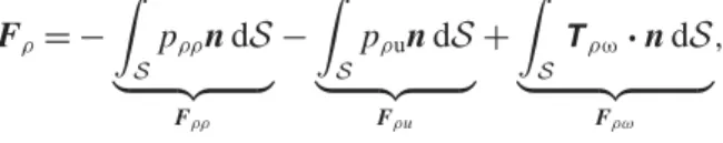
Fρ= F − Fw, as Fρ= − Z S pρρndS | {z } Fρρ − Z S pρundS | {z } Fρu + Z S Tρω· n dS | {z } Fρω , (2.16)
with Tρω= −pρωI + Re−1(∇uρ+ ∇u
T
ρ), the superscript
T denoting the transpose. The
contribution Fρρ in (2.16) may be thought of as an additional Archimedes force due to
the non-zero pressure gradient induced by the deflection of the isopycnals round the
body, while Fρu is an inertial force resulting from the momentum flux associated with
the velocity field uρ when Re 6= 0. Last, pρω= pρ− ( pρρ+ pρu) is entirely determined
by the solenoidal contributions to (2.10). Moreover the divergence-free condition (2.9) combined with the no-slip condition in (2.11) imply (∇uρ+ ∇uTρ) · n = ωρ× n on (S)
(see e.g. equation (A11) in Magnaudet (2011)). Hence Fρω represents the entire force
due to the vorticity ωρ induced by the baroclinic torque.
The two contributions Fρρ and Fρω are the two sides of the same coin, as they both
result from the misalignment between the pressure and density gradients. However, this misalignment manifests itself in two different ways. On the one hand it distorts the vortex lines about the body, which in turn modifies the vorticity, hence the shear
stress at the body surface, yielding the drag contribution Fρω. On the other hand, the
deflection of isopycnals round the body results in the net dragging of a volume of ‘light’ fluid within which the density at every vertical position is smaller than that
of the surrounding fluid. This entrainment, responsible for the drag contribution Fρρ,
is the mechanism on which the semi-empirical modelling effort (Srdic-Mitrovic et al.
1999; Higginson et al. 2003; Yick et al. 2009) has focused up to now.
3. Simulation results
We now apply the above methodology to the flow induced by a settling sphere (from now on, a is the sphere radius). Details about the numerical approach used to solve (2.1)–(2.5) and extensive validation tests are provided in appendix A. We select
Pr =0.7, 7 and 700, corresponding to the diffusion of heat in the atmosphere, and
that of heat and salt in water under standard conditions, respectively. We consider the parameter range 0.05 6 Re 6 100, 0.1 6 Fr 6 10, assuming that the flow is axisymmetric throughout that range. The representativity of this parameter range with respect to field and laboratory conditions, i.e. the relative density range under which gravity/buoyancy-driven bodies may effectively experience O(1)-Froude numbers
when their Reynolds number lies in the above interval, is discussed in appendix B.
3.1. Flow field
Figure 2 displays isopycnals, streamlines and levels of the vertical velocity, u · ez−1,
about the sphere for selected values of Re, Fr and Pr.
When viscous diffusion dominates momentum transport (figure 2a–d), isopycnals
-0.95 -0.50 -0.05 -0.9 -0.5 -0.1 -0.95 -0.50 -0.05 -0.90 -0.41 0.08 Pr = 0.7 Fr = 5 Pr = 0.7 Pr = 700 Pr = 700 8 (a) (b) (c) (d) 6 4 2 0 -2 -4 -0.9 -0.5 -0.1 -0.9 -0.4 0.1 -0.9 -0.4 0.1 -0.8 0.4 1.6 8 (e) (f) (g) (h) 6 4 2 0 -2 -4 -0.9 -0.4 0.1 -0.8 0 0.8 -0.8 0.2 1.2 -1.0 1.5 4.0 8 (i) ( j) (k) (l) 6 4 2 0 -2 -4 R e = 0.05 R e = 5 R e = 100 -4 -2 0 2 4 -4 -2 0 2 4 -4 -2 0 2 4 -4 -2 0 2 4 Fr = 0.5
FIGURE 2. (Colour online) Influence of Re, Fr and Pr on the flow structure. Colours: iso-levels of the vertical velocity, u · ez−1, in the laboratory frame; solid lines: isopycnals,
ρ− z =const. (left half), and streamlines (right half).
enough Pr (figure 2b,d). In this case, the top-down symmetry of the velocity field
is almost unaffected when Fr ≫ 1 (figure 2b), whereas no such symmetry subsists
when Fr . 1 (figure 2d). Instead, for low Fr, a region with upward absolute velocities
u· ez−1 > 0 takes place at some distance downstream of the sphere. This specific
structure is driven by the baroclinic torque which converts the positive radial density gradient encountered within the fluid column dragged by the sphere into a vortex ring with positive azimuthal vorticity, i.e. upward velocities near the symmetry axis. Decreasing Fr and/or increasing Pr increases the curvature of the streamlines
(figures 2b and 2c), which yields closed flow regions (i.e. toroidal eddies) with
size comparable to the body length when the vertical confinement imposed by the stratification is strong enough (figure 2d).
In inertia-dominated situations (figure 2e–l), the lower Fr and the larger Re and
Pr, the thinner the dragged fluid column and the larger the upward velocity on
the wake axis. With Fr = 0.5 and Pr = 700 (figures 2h and 2l), the high-Re wake
structure is dominated by a thin upward jet (Torres et al. 2000; Hanazaki et al.2009a,
2015) with centreline velocities several times larger than the sphere speed. Internal
waves (Mowbray & Rarity 1967) propagating upwards become salient when Fr . 1
(figure 2g–h,k–l). For a given Fr, the size of the closed regions is smaller than in the low-Re regime; for low Fr, they exhibit a V-shape due to the streamwise modulation
of the vertical velocity by the internal waves (figure 2g–h,k–l). The influence of Pr
is weaker than in the low-Re regime, except within the jet region. In line with the
findings of Torres et al. (2000), no standing eddy (which would correspond to vertical
velocities less than −1 in figure 2) exists at the back of the sphere for Re = 100
throughout the explored range of Fr, in contrast with the homogeneous situation in which this structure is present for Re & 10 (Batchelor 1967).
3.2. Buoyancy-induced contributions to the drag
The various contributions to the drag acting on the sphere are shown in figure 3. The
drag is only weakly affected by stratification effects for Fr = O(10), with less than 5 % (respectively 25 %) increase compared to the ‘homogeneous’ drag at Re = 0.05 (respectively 100). In contrast, decreasing Fr to lower values makes the drag increase dramatically whatever Re, especially for large Pr. With Pr = 700 and Fr = 0.5, the drag almost doubles compared to its value in a homogeneous fluid when Re = 0.05, and is eight times larger when Re = 100. Decreasing Pr to 0.7, while maintaining Fr and Re unchanged, reduces the drag enhancement by a factor of 5 (respectively 2) at low (respectively high) Re.
In all cases, the contribution Fρu due to the inertial pressure correction is negative
(i.e. it provides a downthrust) but is negligibly small in magnitude. The reason for this may be qualitatively understood by examining the behaviour of the right-hand side of (2.14), i.e. the momentum flux, in the vicinity of the body surface. As uw and uρ both
obey a no-slip condition on (S), continuity requires that their tangential (respectively normal) component varies linearly (respectively quadratically) with the distance r − 1 to (S) in the immediate vicinity of the latter (r = ||x||). Therefore (uρ+ uw) · ∇uρ+
uρ· ∇uw varies as (r − 1)2 within this surface layer, forcing the momentum flux to
vanish on (S) and be proportional to r − 1 close to it. Consequently the source term in the Poisson equation (2.14) is nearly zero close to (S), and variations of pρu along
the body surface essentially result from the distribution of the momentum flux at some
distance from (S). This non-locality limits the variations of pρu along (S), hence the
magnitude of Fρu. No such effect exists in the case of Fρρ, since the distribution of
pρρ along (S) is mostly driven by the non-zero near-surface density gradients.
When Re is low, the additional Archimedes force Fρρ is also negligible compared
to the vortical contribution Fρω, although its relative magnitude increases with Pr.
Both contributions are of the same order when Re = 100 and Pr is moderate. However,
when Pr is large, Fρω provides again the major part of the extra drag at Re = 100,
being roughly twice as large as Fρρ. These results reveal that modifications of the
vorticity field resulting from the baroclinic torque play a pivotal role in the drag increase throughout the explored Re-range. Conversely, density variations at the body surface play a negligible role at low Re but their relative magnitude gradually increases with the Reynolds number. This state of affairs seriously questions the available attempts in which the stratification-induced drag has been modelled by
0.125 0.25 0.5 Fr Fr 1 2 4 8 0.125 0.25 0.5 1 2 4 8 0.125 0.25 0.5 1 2 4 8 0.125 0.25 0.5 1 2 4 8 0.125 0.25 0.5 1 2 4 8 0.125 0.25 0.5 1 2 4 8 5 4 3 2 1 0 35 25 15 5 -5 2.5 2.0 1.5 1.0 0.5 0 -0.5 25 20 15 10 5 0 -5 1.5 1.0 0.5 0 -0.5 (a) 15 F F®® F®ø F®u 10 5 0 -5 (d) (b) (e) (c) (f)
FIGURE 3. (Colour online) Contributions, as given in (2.16), to the vertical force on the
sphere versus the Froude number for Re = 0.05 (left) and Re = 100 (right) with, from top to bottom, Pr = 0.7, 7 and 700. All contributions are normalized by the ‘homogeneous’ drag force, Fw= Fw· ez at the same Re, so that F · ez/Fw=1 + (Fρρ+ Fρu+ Fρω) · ez/Fw.
evaluating the buoyancy provided by the volume of light fluid dragged by the body,
especially in the low-Re regime (Yick et al. 2009), or for Reynolds numbers of some
units (Srdic-Mitrovic et al. 1999).
4. Stratification regimes and scaling laws for the buoyancy-induced drag
To better understand how Fρω and Fρρ vary with the control parameters, it is
desirable to rationalize the trends revealed by figure 3. Additionally, obtaining explicit scaling laws for these two contributions may allow predictions provided by present numerical results to be extended to a broader range of parameters, especially with
respect to the Reynolds number. To this end, we start from (2.2) and (2.10) and
¶s ¶˚ ¶√ (s) ¶s ¶˚ ¶√ (s) ¶s ¶˚ ¶√ (s) R3 R2 R1 (a) (b) (c)
FIGURE 4. (Colour online) Sketch of the three possible stratification regimes about a unit radius sphere settling at low Reynolds number (ℓν≫1). In (a) the Prandtl number has been selected such that Pr & 1 (since ℓκ. ℓν), while in (b) Pr ≫ 1 (since ℓκ≪ ℓν). The high-Re case is similar, except that ℓν is much smaller than the characteristic body size. vorticity associated with the buoyancy-induced flow in the form
Dwρ Dt − Pe −1∇2ρ= (u ρ+ uw) · ez−1, (4.1) Dwωρ Dt + uρ· ∇ωw− ωρ· ∇uw− ωw· ∇uρ− Re −1∇2 ωρ= Fr−2ez× ∇ρ, (4.2)
where ωρ= ∇ × uρ and ωw= ∇ × uw denote the vorticity associated with the
buoyancy-induced and homogeneous flow fields, respectively, and Dw/Dt≡ ∂t+ uw· ∇ is the
material derivative with respect to the homogeneous flow. Linearization in (4.1) and
(4.2) assumes that ||uρ|| ≪ ||uw||, ||∇uρ|| ≪ ||∇uw|| and ||ωρ|| ≪ ||ωw||. We make use
of the vorticity balance (4.2) instead of the momentum balance (2.10) to avoid having
to discuss the scaling of the pressure term in each regime. The scaling laws for the
buoyancy-induced forces, Fρω and Fρρ stem from the dominant balances in (4.1) and
(4.2), and the characteristics of the undisturbed velocity field, uw. The cornerstone of
the procedure consists in determining the characteristic length scale, ℓs, over which
buoyancy effects generate a velocity disturbance, uρ, of the same magnitude, u, as
the driving ‘homogeneous’ disturbance, uw· ez−1, in the sphere vicinity. These effects
must in principle remain small enough for the linearization that led to (4.1) and (4.2) to be legitimate. By comparing effects of stratification with those of viscosity and diffusivity, which act over length scales ℓν and ℓκ, respectively, three regimes in which
Fρω and Fρρ vary differently with Fr, Re and Pr may be identified, for both low and
high Reynolds number. A schematic view of the corresponding three configurations is
provided in figure 4 in a low-Re case.
4.1. Low-Reynolds-number range
We first consider the low-Re range, in which ℓν= Re−1. Depending on whether Pe
is small (Pr = O(1)) or large (Pr ≫ 1), one then has ℓκ = Pe−1 or Pe−1/3 (Levich
1962; Batchelor 1980). If stratification is strong enough for the condition ℓs≪ ℓν to
be satisfied, inertial terms are negligible in (4.2). Then the balance between buoyancy
and viscous effects reduces to
Re−1∇2ωρ | {z } O(u/ℓ3s) ≈ Fr−2∇ρ × ez | {z } O(ρℓ/ℓs) , (4.3)
so that the density disturbance, ρℓ, associated with the velocity disturbance, u, obeys
ρℓ∼ Fr2Re−1u/ℓ2s. If moreover ℓs ≪ ℓκ (which corresponds to configuration (a) in
figure 4), advective effects are negligible in the linearized density balance (4.1) which then reduces to Pe−1 ∇2ρ |{z} O(ρℓ/ℓ2s) ≈1 − (uρ+ uw) · ez | {z } O(u) . (4.4)
Hence the driving term, 1 − uw· ez, is balanced by diffusive effects, which requires
Pe−1ρℓ/ℓ2s∼ u. Note that the buoyancy-induced advective term, uρ· ez, subsists in (4.4),
as it is assumed to have the same magnitude as the driving term, in contrast with the
settling-induced advective contribution, uw · ∇ρ. The disturbance u being small but
arbitrary, compatibility between (4.4) and (4.3) implies ℓ4
s≈ Fr
2/(PeRe). This defines
a viscous–diffusive regime, which we refer to as R1, characterized by a stratification length scale
ℓs≈ ℓs1≡ (Fr/Re)
1/2Pr−1/4. (4.5)
The relevance of this viscous–diffusive length scale was first recognized by List (1971) and later rediscovered independently by Ardekani & Stocker (2010).
To evaluate Fρω and Fρρ under such conditions, the spatial distribution of the
settling-induced velocity, uw, about the body must be considered. At a distance r
from the sphere centre, the disturbance uw− ez is dominated by the contribution of
the Stokeslet, which makes it decay approximately as r−1 for increasing r. Departures
from this dominant behaviour arise because of the presence of a dipole (required to satisfy the no-slip condition on (S)), and of inertial corrections required for the
solution to be valid throughout the fluid domain, including the outer region r ≫ Re−1
(Batchelor 1967). These additional contributions make the settling-induced velocity
field decay slightly faster than O(r−1), so that we may consider that, for r ≫ 1,
|uw · ez −1| approximately behaves as r−(1+α) with α & 0. The vortical force, Fρω,
scales as the viscous traction at the body surface, Re−1n
· (∇uρ + ∇uTρ). On (S),
||uw− ez|| =1 due to the no-slip condition, whereas at the radial position r = 1 + ℓs1,
||uw− ez|| ≪1 provided ℓs1≫1, owing to the r−(1+α)-decay. From a physical point of
view, assuming ℓs1≫1 implies that we are considering a characteristic stratification
length scale much larger than the body size (or equivalently, that the sphere is seen as a point force). This condition is fulfilled throughout the range covered by the
low-Re computations. The variation δu of ||uw − ez|| from r = 1 + ℓs1 to r = 1 is
then of O(1), and so is that of ||uρ||, due to our definition of the stratification length
scale. Assuming that the above scaling for ℓs1, derived under the assumption u ≪ 1,
holds up to δu = O(1) leads to the conclusion that n · ∇uρ ∼1/ℓs1 on (S). Hence
Fρω∼ (Reℓs)−1, which in the viscous–diffusive R1 regime implies
Fρω≡ Fρω1∼ (FrRe)−1/2Pr1/4. (4.6)
The above result was obtained without considering the contribution of the pressure
component pρω. However the latter exists only to ensure that the velocity field uρ is
solenoidal (i.e. pρω plays the role of a Lagrange multiplier), which implies that its
variations round the body have the same order of magnitude as those of the viscous
traction defined above. Hence the contributions of pρωn and Re−1n· (∇uρ + ∇uTρ)
to Fρω have the same magnitude whatever the Reynolds number (for the same
reason, it is well known (Batchelor 1967) that the surface shear stress (respectively
pressure) provides 2/3 (respectively 1/3) of the drag force on a sphere in the low-Reynolds-number regime, and the same ratios hold in the limit of very large
-2/3 -1/2 -2 -3/2 -1 10-1 100 Fr 101 101 100 10-1 10-2 10-3 10-4 10-5
FIGURE 5. (Colour online) Variations of normalized force components Fρρ · ez/Fw
(triangles, red online) and Fρω· ez/Fw (circles, blue online) in the low-Re regime (Re =
0.05); dash-dotted line: Pr = 0.7, solid line: Pr = 700.
Reynolds numbers for a sphere obeying a shear-free condition, i.e. a bubble with a negligible inner viscosity (Kang & Leal 1988)).
The force component Fρρ is directly proportional to the pressure component pρρ on
(S). From (2.12) and (2.13) one infers that ∇pρρ∼ −Fr−2ρez near the body, so that
the surface value of pρρ scales as Fr−2ρℓz, with z the vertical position with respect to
the sphere centre. Hence one has Fρρ∼ Fr−2ρℓ, with ρℓ evaluated on (S). To estimate
ρℓ, one has to return to (4.4) and make use of the various estimates obtained above,
which yields Pe−1 ∇2ρ |{z} O(ρℓ/ℓ2s1) + uρ· ez | {z } O(ρℓRe ℓ2s1/Fr2) ≈1 − uw· ez | {z } O(r−(1+α)) . (4.7)
Integrating the right-hand side twice and balancing with the diffusive term yields
ρℓ ∼ Peℓs1 (the non-zero, albeit small, α avoids a logarithmic divergence during
this integration). Similarly, provided ℓs1≫1, R
r=1+ℓs1
r=1 |uw· ez−1|dr ≈ 1, so that on
average |uw· ez−1| is of O(1/ℓs1) in between r = 1 + ℓs1 and r = 1. Then, balancing
uρ · ez with this averaged driving term and assuming ρ ≈ 0 for r & 1 + ℓs1 yields
ρℓ∼ Fr2/(Reℓ3s1) at r = 1. Given (4.5), both estimates imply ρℓ∼ (ReFr)1/2Pr3/4 near
the sphere surface, from which one concludes that in the R1 regime
Fρρ≡ Fρρ1∼ Fr−3/2Re1/2Pr3/4. (4.8)
Variations of the buoyancy-induced drag components with the Froude number
predicted by (4.6) and (4.8) are compared with numerical data in figure 5 for
Re = 0.05. Results (4.6) and (4.8) apply provided ℓs1 is much smaller than ℓν
and ℓκ. Hence if Re and Pe are both small, the R1 regime takes place provided
that Fr ≪ min(Re−1Pr1/2, Re−1Pr−3/2), which with Re = 0.05 and Pr = 0.7 implies
approximately Fr ≪ 15. In contrast, if Re is small but Pe is large, the second of the
above bounds changes into Fr ≪ Re1/3Pr−1/6, which with Pr = 700 implies Fr ≪ 0.1 at
in figure 5. Panels (a) and (c) in figure 2correspond to this regime. In figure 5, the
−3/2 slope predicted by (4.8) covers the entire explored Fr-range, whereas the −1/2
slope corresponding to (4.6) is only identified for Fr . 1. Comparing predictions (4.6) and (4.8) indicates that, for a given Fr, the ratio Fρρ1/Fρω1 varies as RePr1/2. Hence
Fρρ is expected to be negligibly small for Re ≪ 1, the buoyancy-induced drag being
dominated by the vortical contribution in this limit. This is confirmed by figure 5
which shows that Fρρ is two orders of magnitude smaller than Fρω throughout the
R1 regime. At the moderate value Pr = 7, the low-Fr low-Re conditions considered in the DNS also belong to the R1 regime. These results may be used to check
the Pr1/4-dependence predicted by (4.6), although the comparison is limited to one
decade (0.7 6 Pr 6 7). As panels (a) and (b) in figure 3 indicate for Fr = 0.1, the
ratio Fρω(Pr =7)/Fρω(Pr =0.7) is close to 2.0, which compares reasonably well
with the expected ratio 101/4≈1.8. The same check can be performed regarding the
Pr3/4-dependence of Fρρ predicted by (4.8), although the numerical values are too
small for the difference to be visible in figure 3. The corresponding ratio is found to
be 5.6, which compares well with the predicted ratio 103/4=5.25. The scaling (4.6) is
similar to that found by Candelier et al. (2014) who computed the buoyancy-induced
correction to the drag using matched asymptotic expansions. These authors made use
of the viscous Richardson number, Ri = Re/Fr2, and found this correction, normalized
by the Stokes drag, to be 0.66(PeRi)1/4. Hence the corresponding force behaves as
Re−1(PeRi)1/4, in line with (4.6).
If stratification is such that ℓκ≪ ℓs≪ ℓν (which corresponds to configuration (b) in
figure 4), the transport of the density disturbance at distances of O(ℓs) from the body
is dominated by advective effects, be the Péclet number small or large. Thus, in the
quasi-steady approximation, the mass balance (4.1) becomes at leading order
uw· ∇ρ | {z } O(ρℓ/ℓs) ≈ (uρ+ uw) · ez−1 | {z } O(u) , (4.9)
so that ρℓ∼ ℓsu, assuming that ||uw|| ≈1 at a distance r ≈ 1 + ℓs from the sphere
centre. Compatibility with the unchanged condition resulting from (4.3) then defines
a viscous–advective regime, R2, characterized by (Chadwick & Zvirin 1974; Zvirin &
Chadwick 1975)
ℓs∼ ℓs2≡ (Fr 2
/Re)1/3. (4.10)
Still assuming ℓs2≫1, repeating the above reasoning implies that the scaling law for
the buoyancy-induced vortical force is now
Fρω2∼ (ReFr)−2/3. (4.11)
Making again use of (4.3), the typical orders of magnitude in (4.9) are uw· ∇ρ | {z } O(ρℓ/ℓs2) − uρ· ez | {z } O(ρℓRe ℓ2s2/Fr2) ≈ uw· ez−1 | {z } O(ℓ−(1+α)s2 ) . (4.12)
Given (4.10), both terms on the left-hand side are of O(ρℓ/ℓs2). Hence with α → 0,
the leading-order balance in (4.12) implies ρℓ∼1 on (S). The reasoning used in the
R1 regime then immediately yields
If Pe ≪ 1 but Pr is large (a combination never met in present computations), the
condition ℓκ ≪ ℓs≪ ℓν implies that the R2 regime takes place if the Froude number
satisfies Pr−3/2Re−1≪ Fr ≪ Re−1. In contrast, ℓ
κ = Pe−1/3 if Pe ≫ 1 (Levich 1962;
Batchelor 1980), in which case the R2 regime takes place if the Froude number
stands in the range Pr−1/2 ≪ Fr ≪ Re−1. With Re = 0.05 and Pr = 700, hence
Pe =35, this condition corresponds to 0.04 ≪ Fr ≪ 20. Variations of Fρω with Fr
in figure 5 suggest that this regime actually takes place only up to Fr ≈ 1 (panel
d in figure 2 corresponds to this regime). Things are less clear at first glance with
Fρρ for which the −2 slope is approximately found only for Fr & 5. The reason is
that this contribution is affected by finite-ℓs corrections when Fr is small enough
because the estimate ρℓ≈1 no longer holds. It may be shown that the most general
prediction for the density disturbance obtained without assuming ℓs2≫1 is actually
ρℓ(r)∼ (ℓs2/r)3. Hence the general scaling for Fρρ2 is Fρρ2∼ Re−1(1 + (Fr2/Re)1/3)−3,
which reduces to (4.13) only in the limit ℓs2≫1. In contrast the general expression
predicts Fρρ2 ∼ Re−1 when ℓs2 is very small, i.e. when Fr ≪ 1. This is why in
figure 5 the negative slope of the corresponding line is seen to decrease with Fr (a
qualitatively similar alteration of (4.8) is expected to take place when ℓs1 ≪1 and
may be computed with similar arguments; however this regime is not reached in
present computations). Comparing (4.11) and (4.13) shows that Fρρ2/Fρω2 varies as
Re2/3 at a given Fr. Hence Fρρ is again expected to be negligibly small for Re ≪ 1 in
the R2 regime, but the ratio Fρρ/Fρω is larger than in the R1 regime, as confirmed
by figure 5. Predictions corresponding to the R2 regime were obtained using matched
asymptotic expansions by Zvirin & Chadwick (1975) who found the drag correction,
normalized by the Stokes drag, to be 1.06Ri1/3 in the limit Pe → ∞. This implies a
Re−1Ri1/3-scaling of the buoyancy-induced drag, equivalent to (4.11).
Finally, an inertial–advective regime, R3, emerges if stratification is so weak
that ℓs ≫ ℓν (hence ℓs ≫ ℓκ, given the range of Pr considered here). Under such
circumstances, which correspond to configuration (c) in figure 4, advection dominates
over viscous effects. Consequently, the relevant quasi-steady approximation of (4.2)
to be considered is at leading order uw· ∇ωρ | {z } O(u/ℓ2 s) + uρ· ∇ωw | {z } O(u/ℓ2 s) − ωρ· ∇uw | {z } O(u/ℓ2 s) − ωw· ∇uρ | {z } O(u/ℓ2 s) ≈ Fr−2∇ρ × ez | {z } O(ρℓ/ℓs) , (4.14)
which implies ρℓ ∼ Fr2u/ℓs. As the relevant density balance is still (4.9), which
imposes ρℓ∼ ℓsu, compatibility implies
ℓs∼ ℓs3≡ Fr, (4.15)
and the reasoning that led to (4.6) immediately yields
Fρω3∼ (FrRe)−1. (4.16)
At r = 1 + ℓs3, the velocity disturbance due to the body motion is governed by
the Oseen equation. Considering moderate Froude numbers such that ℓs& Re−1, we
assume that uw · ez −1 still behaves approximately as r−(1+α) with α & 0 at such
distances from the body, so that the typical orders of magnitude in (4.9) are
uw· ∇ρ | {z } O(ρℓ/ℓs3) − uρ· ez | {z } O(ρℓℓs3/Fr2) ≈ uw· ez−1 | {z } O(ℓ−(1+α)s3 ) . (4.17)
Again this yields ρℓ∼ 1, so that the scaling of Fρρ3 is found to be similar to that of
Fρρ2, viz.
Fρρ3∼ Fr−2. (4.18)
Variations of Fρω shown in figure 5 display the −1 slope predicted by (4.16) for
both Pr = 0.7 and Pr = 700 when Fr & 5. Thus, the R1–R3 and R2–R3 transitions
are found to take place for Fr-values of some units in both cases (panel b in figure 2
corresponds to the lower limit of the R3 regime in the high-Pr case). Mehaddi et al.
(2018) determined asymptotically the first-order drag corrections due to stratification
or inertia effects in the limit Re ≪ 1 and ℓs1 ≫ 1 but did not identify the R3
regime. This is because Fr is much larger than Re−1 there (provided Pr & 1), which
implies Fρω3 ≪1 according to (4.16). Hence the corresponding buoyancy-induced
drag correction is much smaller than the O(1) Oseen inertial contribution, which was the leading-order correction computed in the limit FrRe ≫ 1 by these authors.
To finish with the low-Re range, it is interesting to have a look at the empirical
low-Re buoyancy-induced drag correction proposed by Yick et al. (2009). In this
work, it was suggested that the relative increase of the drag coefficient behaves as
Ri1/2 provided Re is small and Pr is large (their equation (5.2)). This correlation was
based on experimental and numerical results obtained for Pr = 700 with two different Reynolds numbers, Re = 0.05 and 0.5, and Froude numbers up to Fr = 2. With Pr =700 and Re = 0.05, one has ℓν≈20, ℓκ ≈0.3, ℓs1≈0.9 Fr
1/2 and ℓ
s2≈4.5Fr 2/3.
Hence, according to the present analysis, the whole range 0.4 6 Fr 6 2 stands
essentially in the R2 regime. Similarly, with Pr = 700 and Re = 0.5, one has ℓν≈2,
ℓκ ≈0.15, ℓs1≈0.3 Fr
1/2 and ℓ
s2≈2.1 Fr
2/3. Hence data in these series approach the
R1 regime for Fr ≈ 0.4 (since ℓs1 ≈ ℓκ there) and the R3 regime for Fr & 1 (since
ℓs3 ≈ ℓν there) but they also essentially stand in the intermediate R2 regime. As
mentioned above, (4.11) implies that the relative drag increase behaves as Ri1/3 in
this regime, which suggests that, at a given Fr, it should be approximately 2.2 larger for Re = 0.5 than for Re = 0.05 when Fr & 1, in line with the ratio deduced from data
reported by Yick et al. (2009). Conversely, in the R1 regime, equation (4.6) implies
that the relative drag increase is proportional to (Re/Fr)1/2 at a given Pr, so that the
ratio of the two relative drag increases should be close to 3.15 for Fr ≈ 0.4, which is again in agreement with their data. Hence the correlation proposed in Yick et al.
(2009) appears to be an ad hoc approximation which actually mixes two different
asymptotic regimes (see §B.2 in appendix B for more details).
4.2. High-Reynolds-number range
When the Reynolds number is large, ℓν= Re−1/2, owing to the presence of the viscous
boundary layer (hereinafter abbreviated to VBL). In this Re-range, the thickness of the
diffusive boundary layer obeys ℓκ= Re−1/2Pr−1/3 (Acrivos 1960; Levich 1962), since
we are only considering moderate-to-large Prandtl numbers. Although the scalings
Fρω ∼ (Reℓs)−1δu and Fρρ ∼ Fr−2ρℓ derived in §4.1 still apply, the presence of
the VBL, the thickness of which is much smaller than the body radius, prevents the existence of a simple expression for uw about the sphere. Details of the uw-distribution
within the VBL are especially important in the strongly stratified R1 and R2 regimes, since the corresponding stratification length scales are by definition (much) smaller than ℓν. These features make the overall situation less tractable with qualitative scaling
arguments than in the low-Re case, restricting the validity range of the corresponding predictions, especially at low Froude number.
Let us first assume that the Froude number is large enough for the stratification
length scale to be such that ℓs ≫ ℓνMax(1, Pr−1/3). Under such conditions, neither
molecular diffusion nor viscosity affects the buoyancy-induced flow, defining a
high-Re R3 regime. Panels (i) and ( j) of figure 2 provide two examples of this regime.
The corresponding situation is similar to the low-Re R3 regime except that, close to the body, it involves much larger velocity gradients. This makes it necessary to
determine the scaling of ℓs within the VBL. To this end, one has to recognize that,
except in the top region of the sphere where the upward jet originates, variations in directions parallel to the body surface are much slower than in the radial direction. For
this reason one has to distinguish between longitudinal (∇k) and radial (∇⊥) gradient
components, and longitudinal (Ls) and radial (ℓs) buoyancy length scales. One also has
to take into account the fact that uk
w and u
⊥
w are respectively of O(1) and O(ℓν) near
the outer edge of the VBL, owing to continuity. The buoyancy-induced vorticity ωρ
being of O(u/ℓs) within the VBL, the leading-order approximations of (4.1) and (4.2)
for r = O(1 + ℓν) respectively reduce to
uk w· ∇kρ | {z } O(ρℓ/Ls) + u⊥w· ∇⊥ρ | {z } O(ρℓℓν/ℓs) ≈ (uρ + uw) · ez−1 | {z } O(u) , (4.19) uk w· ∇kωρ | {z } O(u/(ℓsLs)) + u⊥w· ∇⊥ωρ | {z } O(u ℓν/ℓ2s) + · · · ≈ Fr−2∇ρ × ez | {z } O(ρℓ/ℓs) . (4.20)
Terms on the left-hand side have the same magnitude provided that Ls= ℓ−1ν ℓs, and
compatibility between (4.19) and (4.20) implies that, close to the body,
ℓs∼ ℓs3≡ ℓνFr = Re−1/2Fr. (4.21)
It may then be concluded that the condition ℓs ≫ ℓνMax(1, Pr−1/3) defining
the high-Re R3 regime corresponds to values of the Froude number such that
Fr ≫Max(1, Pr−1/3), i.e. Fr ≫ 1 since we are not considering low Prandtl numbers. As
ℓs3/ℓν≫1, the driving term in (4.19) is small at r ≈ 1 + ℓs3, so that the approximation
δu≈1 holds in between (S) and r = 1 + ℓs3. Hence the scaling Fρω∼ (Reℓs)−1 derived
in §4.1 is still valid, implying
Fρω3∼ Fr−1Re−1/2. (4.22)
Within the VBL, spatial variations of the forcing term 1 − uw· ez in (4.7) deeply
differ from the low-Re case. They now correspond to a boundary-layer-type solution,
F(η), with η = (r − 1)/ℓν, supplemented by wake corrections. Unfortunately, the
explicit form of F(η) is unknown except in the limit η ≪ 1, especially in the wake region where most of the distortion of the isopycnals takes place. For this reason,
a direct qualitative integration of (4.19) from r = 1 to r = 1 + ℓs3 is not possible.
This is why one has to resort to a different strategy to estimate Fρρ3. The alternative
approach calls on a Lagrangian energy balance over an infinitesimal fluid element, from its initial arbitrary position to its final position close to the body surface. This
balance is established in appendix C. Its final outcome is (C 6) which allows us to
conclude that, close to the body but at distances from its surface larger than the VBL thickness, ρℓ∼ Fr(1 + O(Re−1)). Since pρρ scales as Fr−2ρℓz on (S) (see §4.1), one
has in this regime and provided Re ≫ 1
-2/3 -1/2 -1 -1 -1 102 101 100 10-1 10-2 10-1 100 Fr 101
FIGURE 6. (Colour online) Variations of normalized force components Fρρ · ez/Fw
(triangles, red online) and Fρω· ez/Fw (circles, blue online) in the high-Re regime (Re =
100); dash-dotted line: Pr = 0.7, solid line: Pr = 700.
Predictions (4.22) and (4.23) are confirmed in figure 6 in which both drag components
are seen to exhibit a −1 slope beyond Fr ≈ 1 for Pr = 0.7 and, with some slight
deviations, for Pr = 700. A crucial property revealed by (4.23) is that Fρρ3 does not
depend on Re, while according to (4.22) Fρω3 still varies as Re−1/2. This is reflected
in the relative magnitude of the two drag components which is now of O(1) for Re =
100, although Fρω is still typically twice as large as Fρρ as soon as Fr is of O(1) or
larger (see also panels d and f in figure 3). This is in stark contrast with the low-Re
regime in which the vortical contribution is always responsible for almost the entire buoyancy-induced drag increase.
Let us now examine the two low-Fr regimes. The viscous–diffusive R1 regime takes place if ℓs1 ≪ min(ℓν, ℓκ), i.e. Fr ≪ min(1, Pr−1/6), with ℓs1 still given by (4.5).
Since Pr−1/6 ≈0.3 for Pr = 700, this regime may only be observed for Pr = 0.7
and Pr = 7 in present computations (figure 2(k) stands near the higher-Fr bound of
this regime). The reasoning that led to (4.6) remains unchanged. Despite the VBL
structure, the estimate δu = O(1) in between r = 1 and r = 1 + ℓs1 still holds, provided
ℓs1, hence Fr, is ‘not too small’. This may be seen by assuming that the flow near
the sphere surface may locally be roughly approximated by Blasius’ boundary-layer solution over a flat plate. Then, considering for instance Fr = 0.1 and Pr = 0.7, one has ℓs1/ℓν= η ≈0.35, a position at which the local tangential velocity predicted by Blasius’
solution is approximately 55 % of the free-stream velocity. Hence u has changed from u =1 at the sphere surface to u ≈ 0.5 at r = 1 + ℓs1 for the shortest ℓs1, which makes
the approximation δu = O(1) still reasonable. Consequently the scaling law (4.6) for
Fρω1 is unchanged at leading order. This is confirmed in figure 6 in the subrange
0.1 6 Fr . 0.3, in which the expected −1/2 slope is observed. This is also confirmed
regarding the Pr1/4-dependence, by comparing results displayed in panels (d) and (e)
of figure 3. Indeed, for Fr = 0.1, Fρω(Pr=7)/Fρω(Pr=0.7) ≈ 1.85, which is close
to the expected ratio 101/4≈1.8. Similar to the R3 regime, one has to rely on the
Lagrangian energy balance established in appendix C to estimate Fρρ1, since most
In this case, equation (C 6) implies ρℓ ∼ Fr(1 + O(Re−1/2)) near the body surface,
which leaves the leading-order estimate for Fρρ unchanged, viz.
Fρρ1∼ Fr−1. (4.24)
The Fr−1-behaviour is observed in figure 6 for Pr = 0.7 and Fr . 0.3. Again, the
high-Re predictions suggest that the vortical component to the buoyancy-induced
drag decreases as Re−1/2, and the Archimedes-like component is independent of
the Reynolds number. However, while the former is still larger than the latter for
Re =100 in the case of the R3 regime, the situation is reversed in the R1 regime, the
ratio Fρω/Fρρ being close to 0.5 for Fr = 0.1 according to figure 6. This situation is
also to be compared with the low-Re R1 regime in which this ratio is typically two
orders of magnitude larger. Finally, it must be noticed that, although Fρω1 varies with
the Prandtl number according to (4.6), (4.24) predicts that Fρρ1 does not. Comparing
panels (d) and (e) in figure 3 confirms that increasing Pr from 0.7 to 7 leaves Fρρ
unchanged in the low-Fr range.
The R2 regime also exists when Pr ≫ 1, provided the Froude number is such that ℓκ≪ ℓs≪ ℓν. If these inequalities hold, the relevant orders of magnitude in the
vorticity equation arise from (4.3), implying ρℓ∼ Fr2Re−1u/ℓ2s. In the density equation,
they would be similar to those resulting from (4.19) if ℓs2 were only ‘slightly smaller’
than ℓν, since the two components of uw were evaluated near the outer edge of the
VBL in (4.19). If this were the case, the density equation would imply ρℓ∼ (ℓs/ℓν)u.
However the decrease of both components of uw with η cannot be ignored if ℓs2 is
significantly smaller than ℓν, i.e. η(ℓs2)≪1. In particular, Blasius’ solution suggests
that ||u⊥
w|| varies approximately linearly (respectively quadratically) with η in the
range 0.2 6 η 6 0.7 (respectively 0 < η < 0.2). Hence in the former range, ||u⊥
w|| ∼ ℓs,
so that the corresponding advective term in (4.19) is of O(ρℓ), and the balance with
the right-hand side implies ρℓ ∼ u. Although there is no reason to expect uw to
vary as a power law of η for η > 0.2 (Blasius’ solution rather suggests a hyperbolic tangent behaviour), the above two distinct scalings arising from the density equation
may be qualitatively gathered in the form ρℓ ∼ (ℓs/ℓν)βu, with β decreasing from
1 to 0 as ℓs/ℓν decreases from O(1)- to O(10−1)-values. Compatibility between the
leading-order balances provided by (4.3) and (4.19) then yields
ℓs∼ ℓs2≡ Re−1/2Fr2/(2+β), (4.25)
which predicts the R2 regime to take place in the Fr-range Pr−1/3≪ Fr ≪1, since
the lower bound of ℓs2 is reached with β ≈ 0. We previously showed that the estimate
δu= O(1) is still legitimate for stratification lengths significantly smaller than ℓν. So,
in the above range of ℓs/ℓν, the vortical component of the buoyancy-induced drag may
still be considered to scale as Fρω2∼ (Reℓs2)−1, i.e.
Fρω2∼ Re−1/2Fr−2/(2+β). (4.26)
Therefore the above reasoning predicts that variations of Fρω in the high-Re R2 regime
should be close to a power law with an exponent standing in between −2/3 and −1, depending on the actual ratio ℓs2/ℓν. For Re = 100 and Pr = 700, ℓκ≈0.1ℓν and, with
β=0, Pr−(2+β)/6= Pr−1/3≈0.11. Consequently the R2 regime is expected to cover a
limited extent in the range 0.1 ≪ Fr ≪ 1. A subrange with a slope corresponding to an
exponent in between −2/3 and −1 is observed in the corresponding plot of figure 6,
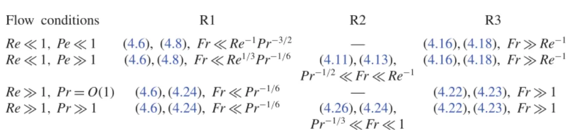
Flow conditions R1 R2 R3 Re ≪1, Pe ≪ 1 (4.6), (4.8), Fr ≪ Re−1Pr−3/2 — (4.16), (4.18), Fr ≫ Re−1 Re ≪1, Pe ≫ 1 (4.6), (4.8), Fr ≪ Re1/3Pr−1/6 (4.11), (4.13), (4.16), (4.18), Fr ≫ Re−1 Pr−1/2≪ Fr ≪ Re−1 Re ≫1, Pr = O(1) (4.6), (4.24), Fr ≪ Pr−1/6 — (4.22), (4.23), Fr ≫ 1 Re ≫1, Pr ≫ 1 (4.6), (4.24), Fr ≪ Pr−1/6 (4.26), (4.24), (4.22), (4.23), Fr ≫ 1 Pr−1/3≪ Fr ≪1
TABLE 1. Domains of existence of the various stratification regimes. Numbers in each row refer to the equation providing the corresponding scaling law for Fρω and Fρρ, respectively. The bounds of some regimes have been simplified by considering only Pr in the range [1, ∞].
The situation regarding the determination of the Archimedes-like component is similar to that discussed in the R1 regime, so that the scaling (4.24) applies to Fρρ2.
In figure 6, the slope of the Fρρ-curve corresponding to Pr = 700 is observed to
change for Fr ≈ 0.3, similar to that of Fρω. For lower Fr, this slope is close to −1
as predicted by (4.24). Similar to the other two high-Re regimes, the scaling (4.26)
predicts that Fρω2 decreases as Re−1/2, while Fρρ2 no longer varies with the Reynolds
number. However, figure 6 shows that the former is still approximately twice as large
as the latter for Re = 100, similar to the behaviour observed in the R3 regime. 4.3. Discussion
Table 1 summarizes the predicted domain of existence of the various asymptotic
regimes derived in § §4.1 and 4.2. It has to be noticed that, while the low-Re R1
and R2 regimes may be associated with stratification lengths significantly larger
than the body even at low Fr (thanks to the Re−1/2 and Re−1/3 dependencies of
ℓs1 and ℓs2, respectively), this is by no means the case at high Reynolds number.
Rather, the high-Re R1 and R2 regimes correspond to situations in which the flow structure in the vicinity of the body is deeply affected by stratification, as may be realized by coming back to the longitudinal and radial buoyancy scales introduced in §4.2. As deduced from (4.19) and (4.20), Ls= ℓν−1ℓs, i.e. Ls∼ Fr1/2Pr−1/4 in R1
and Ls∼ Fr2/(2+β) in R2, with 0 6 β 6 1. According to the bounds established for
these two regimes, this implies that the longitudinal scale is such that Ls≪ Pr−1/3
in R1 and Pr−1/3 ≪ L
s≪1 in R2 whatever β. Hence in both cases, Ls is smaller
than unity, so that the characteristic scale of buoyancy effects in directions parallel to
(S) is smaller than the body scale. In other words, in these high-Re low-Fr regimes,
stratification effects are strong enough to impose a vertical layering of the flow within the boundary layer at scales smaller than the body size.
Nevertheless, the most noticeable point regarding high-Re predictions is that Fρρ
is expected to become independent of the Reynolds number in all three regimes
while Fρω always behaves as Re−1/2, as does the ‘homogeneous’ drag, Fw. The
predicted difference in the high-Re behaviours of Fρω and Fρρ is confirmed in
figure 7 where their variations with Fr, normalized by those of Fw, are compared at
two Reynolds numbers, Re = 50 and 100. Figure 7(a) confirms that Fρω/Fw tends
to become independent of Re, especially when stratification effects are large: no significant variation of the normalized force is observed for Fr 6 5 (respectively 62)
10-1 100 Fr 101 102 (a) 101 100 10-1 10-2 10-1 100 Fr 101 102 (b) 101 100 10-1 10-2
FIGURE 7. (Colour online) Variations of the normalized force components from Re = 50
(pale lines, yellow online) to Re = 100 (dark lines, blue online). (a) Fρω/Fw; (b) Fρρ/Fw.
Dash-dotted lines: Pr = 0.7, solid lines: Pr = 700.
still increasing with Re whatever Fr and Pr. Since Fw∼ Re−1/2, the normalized Fρρ
component is expected to grow as Re1/2, i.e. to increase by a factor of approximately
1.4 from Re = 50 to Re = 100. The order of magnitude of the observed increase is consistent with this estimate.
This critical difference between the low- and high-Re scalings suggests that,
although the vortical contribution Fρω generally dominates the stratification-induced
drag up to Reynolds numbers of O(102), the extra Archimedes force F
ρρ becomes the
dominant contribution when Re becomes very large. However, this high-Re prediction must of course be taken with some caution since the analysis carried out here assumes that the flow is steady and axisymmetric, which is unlikely to be the case when Re → ∞.
Numerical results provided in §3 and scaling laws derived in §4 may be combined
to obtain predictions of the drag increase, hence of the reduction of the settling/rising speed, beyond the bounds of the Reynolds-number range explored computationally here. To this end, one must first refer to table 1 to identify the relevant stratification
regime. With this information, the relevant equations in §4 provide the scaling laws
for Fρω and Fρρ. The missing pre-factors are finally obtained by examining the
numerical data relevant to that regime in figure 3. Examples of this extrapolation
strategy are provided in appendix B in real flow configurations with settling Reynolds
numbers typically two orders of magnitude beyond the upper and lower bounds considered in the simulations, respectively. Predictions obtained through this procedure are shown to agree quantitatively well with experimental data, suggesting that this extrapolation strategy is valid, even under conditions in which the instantaneous
flow is presumably no longer axisymmetric (Akiyama et al. 2019) and small-scale
turbulence is present.
5. Concluding remarks
In this paper, we derived a rational splitting procedure of the flow field aimed at disentangling the various physical effects that contribute to produce an extra drag on bodies settling with a constant speed in a linearly stratified fluid. This splitting identifies three distinct contributions, out of which two dominate the buoyancy-induced drag. One is due to the alteration of the flow structure by stratifications effects, and
results in an extra stress at the body surface originating in the vorticity generated by the baroclinic torque. The other is an Archimedes-like force due to the non-uniform pressure distribution resulting from the density disturbance, i.e. the distortion of the isopycnals, at the body surface. We applied this splitting scheme to a series of direct
simulations spanning three decades of Reynolds number, from viscosity-dominated
to inertia-dominated regimes. Similarly, we considered Prandtl numbers ranging from O(1)-values typical of gases to the value Pr = 700 characterizing the diffusion of salt in water. While the drag is only weakly affected by stratification effects for Fr = 10
whatever the Reynolds and Prandtl numbers, its increase is significant even for Froude
numbers of some units when Re ≪ 1, and exceeds by far the ‘homogeneous’ drag for Fr . 1 when Re ≫ 1. The relative magnitude of the two buoyancy-induced drag components varies with the flow parameters but the former dominates whatever Pr when Re is low, and at least up to Re = O(102) when Pr is large. This conclusion
clearly challenges the possibility of deriving regime-independent models based on a well-defined ‘entrained’ volume of fluid to predict the drag of light settling bodies and particles, especially in the ocean.
To unravel the variations of the two dominant contributions to the drag increase, we derived their scaling laws by considering the leading-order balance resulting from the governing equations. We identified the existence of three different stratification
regimes at both low and high Reynolds number, depending on the strength of
stratification compared to that of viscous and diffusive effects. This yields a total of twelve scaling laws, the predictions of which are supported by the numerical results.
Although present computations span a limited range in Reynolds number, their
bounds are sufficiently far apart to provide quantitative predictions corresponding to viscous-dominated and inertia-dominated regimes, respectively. Obviously, the scaling laws do not suffer from the same limitation with respect to the Reynolds number. This is why, as we showed on several real examples, they may be combined with the numerical results to obtain quantitative predictions of the drag increase for Reynolds numbers at least two orders of magnitude beyond the bounds considered in the computations.
Present results were obtained assuming a prescribed settling speed. However, they can be used to predict the settling speed of gravity-driven bodies for which the drag and net weight are in balance, provided acceleration effects are small and the path remains approximately vertical. Under such conditions, results provided in
§§3 and 4 may be combined in the way discussed in appendix B to determine the
ratio KS(Re, Fr) = C
D(Re, Fr)/CHD(Re) of the actual drag coefficient corresponding
to the set of parameters (Re, Fr) to its ‘homogeneous’ counterpart, CH
D(Re). This
determination requires an iterative process since the body speed, hence Re and Fr, is unknown. Once this process is converged, the vertical position of the body centroid may be predicted as a function of time. Additionally, moderate acceleration effects can be taken into account in a semi-empirical manner by incorporating the inertia force due to the body inertia and the added-mass force evaluated with the reference
fluid density ρ0 in the vertical force balance. Numerical results discussed in §3 are
restricted to the specific case of a sphere. In contrast, the scaling laws derived in
§4 are not, since the derivation only involves properties of the far-field flow at low
Reynolds number, and local properties of the boundary layer at high Reynolds number. Consequently, the strategy used here straightforwardly generalizes to arbitrarily shaped bodies as far as the body does not rotate. For instance, in the case of a body with no axial symmetry about the vertical direction, separate computations with a prescribed velocity along every relevant direction of space must first be performed to compute