BeeCluster: drone orchestration via predictive optimization

BeeCluster: drone orchestration via predictive optimization

The MIT Faculty has made this article openly available.

Please share

how this access benefits you. Your story matters.

Citation

He, Songtao et al. "BeeCluster: drone orchestration via predictive

optimization." 18th Annual International Conference on Mobile

Systems, Applications, and Services, June 2020, Toronto, Canada,

Association for Computing Machinery, June 2020. © 2020 ACM.

As Published

http://dx.doi.org/10.1145/3386901.3388912

Publisher

Association for Computing Machinery (ACM)

Version

Author's final manuscript

Citable link

https://hdl.handle.net/1721.1/128699

Terms of Use

Creative Commons Attribution-Noncommercial-Share Alike

BeeCluster: Drone Orchestration via

Predictive Optimization

Songtao He

_{, Favyen Bastani}

_{, Arjun Balasingam}

_{, Karthik Gopalakrishnan}

_{, Ziwen Jiang}

_,

Mohammad Alizadeh

_{, Hari Balakrishnan}

_{, Michael Cafarella}

_{, Tim Kraska}

_{, Sam Madden}

_{MIT CSAIL,}

_MIT

1

_{{songtao, favyen, arjunvb, ziwenj, alizadeh, hari, michjc, kraska, madden}@csail.mit.edu}

_{[email protected]}

ABSTRACT

The rapid development of small aerial drones has enabled numerous drone-based applications, e.g., geographic map-ping, air pollution sensing, and search and rescue. To assist the development of these applications, we propose BeeClus-ter, a drone orchestration system that manages a fleet of drones. BeeCluster provides a virtual drone abstraction that enables developers to express a sequence of geographical sensing tasks, and determines how to map these tasks to the fleet efficiently. BeeCluster’s core contribution is predictive op-timization, in which an inferred model of the future tasks of the application is used to generate an optimized flight and sensing schedule for the drones that aims to minimize the total expected execution time.

We built a prototype of BeeCluster and evaluated it on five real-world case studies with drones in outdoor environments, measuring speedups from 11.6% to 23.9%.

1.

INTRODUCTION

Rapid progress in the development of small aerial drones has enabled numerous aerial sensing applications, including infrastructure and agricultural inspection [19, 27, 16, 7, 37], air pollution sensing [42, 43, 8, 35], car-tography and geographic mapping [31, 24], traffic mon-itoring [32], disaster relief [6, 33], and search and res-cue [14]. However, developing auto-pilot applications that control a fleet of drones to perform complex sens-ing tasks is often challengsens-ing. As a result, most drones today are manually flown by individual pilots or by sim-ple auto-pilot applications [3, 4] that can only handle static tasks, which is impractical for applications that need to react with the environments [18], such as local-izing the source of air pollution or searching a target in an unknown environment.

To simplify multi-drone application development and deployment, we propose BeeCluster, a drone orchestra-tion system that manages a fleet of drones on behalf of an application. In BeeCluster, application developers write their program for virtual drones. The framework then determines how to schedule the drones to mini-mize the application execution time. At the heart of

BeeCluster is predictive optimization, in which the run-time framework builds a model to forecast future ap-plication tasks, and uses these forecasts to optimize its route planning.

Prior Work: Prior drone orchestration platforms [40, 30, 25, 26, 48] typically adopt a location-oriented pro-gramming model, where developers provide a set of loca-tions and associated acloca-tions, e.g., take photos at specific locations. The system then determines an efficient route to visit all these locations with the available drones, and dispatches the drones to execute the application. A key limitation in all these systems is that they only take into account the current set of requests from the appli-cation for route planning. Even frameworks that allow applications to issue new requests dynamically [30] are myopic, and plan routes based only on the current re-quests at any point in time. By contrast, predictive op-timization considers both the current requests and the application’s likely future requests in the route plan-ning process. In particular, many applications generate new requests once a given sensing task is complete, or cancel a request based on the results of a current task. BeeCluster accounts for these likely future actions in the planning process.

The Opportunity: As an illustrative example, con-sider an application with the active sensing loop shown in Figure 1. The algorithm starts with three initial lo-cations A, B, C. In line 3, the algorithm collects sensor readings from these three locations. Then it updates the three locations based on the sensor readings and proceeds to a new iteration. This basic algorithm repre-sents a category of iterative, active sensing applications, e.g., using gradient descent to localize the source of air pollution [49]. Let An, Bn, Cn denote the locations of A, B, C at line 3 in the n-th iteration.

Consider the scenario in Figure 2 where we wish to run this application using one drone. When the program first reaches line 3, the orchestration system dispatches the drone to visit locations A1, B1, C1. At this time, any orchestration system that only considers the current set of requests, i.e., A1, B1, C1, yields two equivalent routes: A1 → B1 → C1 or A1 → C1 → B1. However, these

1 A,B,C = initial locations 2 while True:

3 values = SenseAtLocations({A,B,C})

4 A,B,C = Update(A,B,C,values)

Figure 1: The pseudo code of an active sensing loop.

B1 A₁ C₁ B₂ A2 C2 Drone B1 A₁ C₁ B₂ A2 C2 Drone

Best Case Worst Case

Figure 2: Possible routes in the best case and the worst case using existing drone orchestration systems

two routes are not equivalent if we consider multiple iterations of the program. If we choose the route A1→ B1→ C1, then in the second iteration, the drone needs to fly from C1 to A2 to start the new iteration (the worst case in Figure 2). However, if we choose the route A1→ C1→ B1, then in the second iteration, the drone only needs to fly from B1to A2to start the new iteration (the best case in Figure 2). In this example, the worst case can take 50% more flying time compared to the best case. However, this optimization is possible only if we consider future requests.

We find there are many drone applications that could benefit from predictive optimization. We provide more examples in Section 2.

Challenges: Making drone orchestration systems pre-dictive is not trivial. On the surface, predicting future application requests appears to require an accurate un-derstanding of application semantics and goals. A naive solution to circumvent this challenge is to provide primi-tives for application developers to explicitly declare pos-sible future requests, or take over the route planning entirely. However, this shifts the burden to application developers, and largely eliminates the advantages of the drone orchestration systems. Thus, we seek a predictive optimization method that does not require developer as-sistance.

Our Approach and Contributions: Our approach is inspired by the branch prediction in CPUs [38], where the CPU predicts the branches and prefetches poten-tial next instructions to speed-up execution. These pre-dictive optimizations happen without the application changes. The predictive optimization technique we de-velop for drone optimization works similarly.

BeeCluster has two main components, the API and the runtime. The API provides a virtual-drone pro-gramming interface to express a wide range of complex drone applications in a compact and flexible way. The runtime interprets the application’s logic as a dynamic

task graph (DTG) and stores the DTG of each exe-cution. While running, BeeCluster uses the historical DTGs as well as the current DTG to forecast the fu-ture behaviour of the application (task creations and cancellations). Then, BeeCluster uses this predicted in-formation to minimize the expected execution time.

We have implemented BeeCluster and describe five case studies built atop it, including road mapping, Wi-Fi mapping and hotspot localization, and continuous object tracking. We found that the BeeCluster API is conveniennt to use and that predictive optimization speeds-up execution time by between 11.6% and 23.9% in these case studies.

2.

MOTIVATING EXAMPLES

In this section, we show five examples to motivate the benefit of predictive optimizations and the API pro-posed in BeeCluster. Each example represents a com-mon application pattern.

2.1

Benefits of Predictive Optimization

Example 1: Speculative Execution. Consider

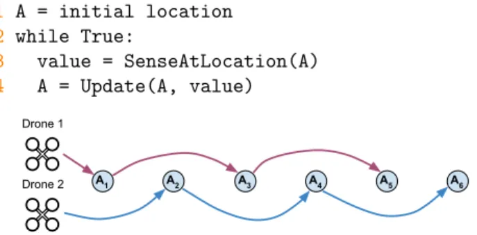
the simple active sensing loop shown in Figure 3. In each iteration, the algorithm senses data at location A. Then, the algorithm uses the data to compute the next location to sense data.

Now suppose we have two drones for this application. Current systems will use only one drone on this appli-cation at any given time because only one request is outstanding. 1 A = initial location 2 while True: 3 value = SenseAtLocation(A) 4 A = Update(A, value) Drone 1 A1 A2 A3 A4 A5 A6 Drone 2

Figure 3: Example of an active sensing loop that can be optimized by speculative execution

By contrast, BeeCluster forecasts the future requests of an application. When there are spare drones in the system, BeeCluster dispatches drones to the locations of the predicted requests, a form of speculative execution. Figure 3 shows the traces of the speculative execution on this application with two drones. This strategy overlaps the flying time of one drone with sensing time of another and thus reduces the total execution time.

We find that the code structure in Figure 3 is com-mon in many drone applications, such as localizing the source of air pollution via gradients [49] and mapping trails or roads using iterative tracing [10]. BeeCluster

is able to apply this optimization without requiring any changes to application code. We performed an eval-uation with a road mapping application that maps a newly constructed road by iteratively tracing the road, and found that this strategy reduces the execution time by 21.3% (case study 1 in Section 5.1.1).

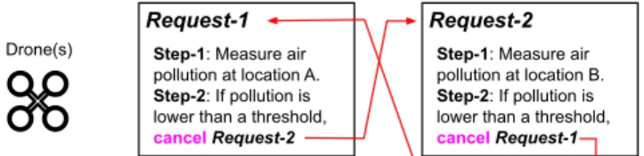
Example 2: Dynamic Request Cancellation.

Besides the dynamic request generation in the active sensing examples, the opposite behaviour, dynamic re-quest cancellation, is also common in many applications. We show an example in Figure 4. The algorithm needs to measure air pollution at two locations. However, once one location is visited, the application may cancel the sensing request at the other location depending on the first value.

Drone(s) Step-1: Measure air

pollution at location A.

Step-2: If pollution is

lower than a threshold,

cancel Request-2 Request-1

Step-1: Measure air

pollution at location B.

Step-2: If pollution is

lower than a threshold,

cancel Request-1 Request-2

Figure 4: Example of dynamic request cancellation. The optimal strategy in this example depends on the prediction of the if branch at Step-2. BeeCluster fore-casts the potential cancellation for each active request in the system. Then the scheduler can use this fore-cast information to optimize the route. Examples of applications that can benefit from this optimization in-clude Gaussian-process-based active information gath-ering [36, 44, 45] for magnetic field, air pollution sensing, wireless signal strength measurement, and exploration in unknown environments [12].

We evaluated an application that maps the Wi-Fi sig-nal strength through Gaussian process (using request cancellations), showing a 23.8% execution time reduc-tion with BeeCluster (case study 2 in Secreduc-tion 5.1.2).

Example 3: Efficient Routing. As noted in the introduction and shown in Figures 1 and 2, knowledge of the future task graph allows BeeCluster to compute the optimal path that minimizes execution time. We evaluated an application that localizes a Wi-Fi hot-spot through gradient descent, finding that BeeCluster’s pre-dictive optimization approach improves performance by 11.6% (case study 3 in Section 5.1.3).

2.2

Benefits of the BeeCluster API

Example 4: Fine-Grained Multiplexing. We

find that programming APIs in existing drone orches-tration systems often bind a virtual drone to a physical drone at task level. The BeeCluster API provides a way to define the binding relationship between virtual drones and physical drones in a precise and fine-grained way, enabling action-level scheduling. For example, consider a delivery task that requires a drone to fly from A to B. In action-level scheduling, the drone assigned to this

task can also perform other tasks, e.g., taking a photo, along the way from A to B. BeeCluster’s API allows de-velopers to describe the logic in this example through a fine-grained binding relationship definition (see Section 3.2.2), enabling fine-granularity action-level multiplex-ing.

We performed an evaluation with a proof-of-concept scenario which involves three simple applications, show-ing the fine-grained multiplexshow-ing can improve the per-formance by 19.1% (case study 4 in Section 5.2.1).

Example 5: Continuous Operation. Consider

the problem of continuously tracking one or more mov-ing vehicles in a city. Because BeeCluster can predict the locations where an algorithm needs to visit in the future, it can dispatch another drone in advance to the location where the original drone may run out of its bat-tery. Then, the original drone hands off the operation to the new drone right before it runs out of battery. Al-though the hand-off may incur a short delay, it is likely that an operation such as object tracking can still pro-ceed normally. We demonstrate the effectiveness of this feature in Section 5.2.2 (case study 5). Although ex-isting drone orchestration systems promise to provide functional virtualization over many physical drones, the time scale of a single continuous operation is still limited by the battery-time of a single drone.

3.

DESIGN

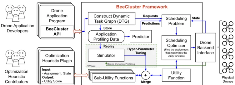
Figure 5 provides an overview of the BeeCluster archi-tecture. The design of BeeCluster is driven by two goals: first, the system should be flexible enough to accurately express a wide variety of drone application logic, and second, the system should be able to effectively opti-mize applications transparently, i.e., without requiring code changes.

To achieve the first goal, we propose the BeeCluster API (Section 3.1). The second goal is challenging for two reasons. First, many optimization solutions require application-specific knowledge that cannot be obtained easily. Second, the optimization is often application-specific, making it challenging to develop a unified ap-proach to optimize different applications.

To overcome these challenges, BeeCluster uses two ideas. First, it models the application’s future behavior as a dynamic task graph (DTG) constructed from the running application. The BeeCluster API makes it pos-sible to do this without application developers needing to codify future behavior. The DTG captures all the necessary information about the application. BeeClus-ter stores both the DTGs from past runs and the par-tially constructed DTG of the current run as profiling data for the application. Then, BeeCluster forecasts the application’s future behaviour by matching the current DTG with previous DTGs. We describe the details of the DTG and the forecast method in Section 3.2.

BeeCluster Framework Drone Application Program BeeCluster API Construct Dynamic Task Graph (DTG) Drone Application Developers Application Profiling Data Optimization Heuristic Contributors Optimization Heuristic Optimization Heuristic Optimization Heuristic Plugin Input: - Assignment, State Output: - Utility Score Drone Backend Interface Simulator Utility Score Scheduling Optimizer

(Find the assignment that maximizes the

utility function) Store Replay Hyper-Parameter Tuning Scheduling Problem Requests Predictions Utility Function +

Utility Score_{Utility Score} Sub-Utility Functions

Drone Dynamic Profiling

Physical Drones Predictor Offline Merge State

Figure 5: Overview of BeeCluster Drone Orchestration Framework

Second, rather than providing a single optimization model for all applications, BeeCluster adopts the instantaneous-assignment [23] scheduling model and provides an ex-tensible platform to support different optimization heuris-tics as plugins. Here, the optimization heurisheuris-tics are used to determine the best instantaneous-assignment of tasks to drones at any point in time. For example, one optimization heuristic could prefer to always dispatch drones to their nearest tasks, and in multi-drone sce-narios, one optimization heuristic could prefer to scatter the drones over the region of interest. Thus, BeeClus-ter is not a fixed collection of optimization heuristics. Instead, it provides a common interface that makes it easy to add new optimization heuristics as plugins. At runtime, BeeCluster considers all possible optimization heuristics and selects the best weighted combination of different heuristics via off-line application replay in a simulator (Section 3.3).

3.1

Programming Model (BeeCluster API)

The API allows developers to describe their appli-cation logic through a DTG-based imperative program-ming model. It also allows developers to explicitly define the precise binding relationship between virtual drones and physical drones, e.g., some actions must be done on one physical drone sequentially, while some other actions can be done with multiple physical drones in parallel.

3.1.1

Basic Primitives

We show the basic primitives of the BeeCluster API in Table 1. The API has two basic building blocks, actions and tasks.

Action. An action is a basic drone operation such as taking a photo or flying to a location. The non-blocking property of the action primitive described in Table 1 enables action batching, allowing the scheduler to consider a whole batch of the actions together, rather

than processing them one-by-one.

Task. A task contains an ordered sequence of ac-tions and maintains the context of a virtual drone; when there are two consecutive actions such that action-1 is flying to location A, and action-2 is taking a photo, the BeeCluster runtime will update the location of the vir-tual drone after action 1 and interpret the second action as taking a photo at location A.

Developers use newTask() create new tasks. Task creation is non-blocking; the blocking (synchronization) only happens when the execution result of a task is re-quired by another statement, i.e., a statement that de-pends on the execution result of the task. In BeeClus-ter, each task corresponds to an independent thread, and the thread can be executed in parallel with other threads when there are available drones. The task prim-itive allows developers to describe independent action sequences, e.g., that the application needs to take pho-tos at a set of locations, but the order of execution does not matter. In this case, traveling to a location and taking a photo would be a single task, and there would be one task for each location in the set.

Developers can use cancelTask() to cancel tasks spec-ified by the task handlers.

3.1.2

Binding Relationships

The developers can define the binding relationship of the actions within a task. The binding relationship pro-vide a way to control the mapping of virtual drones to the physical drones. BeeCluster supports four binding relationships defined by the combinations of two flags.

SameDrone Flag (SmDrn). When the SameDrone flag is set to be True, all the actions within the task need to be done on one physical drone. Otherwise, the ac-tions within the task can be mapped to different physical drones.

Interrupt-Name Description

h=act(args) Execute the action defined by args on a drone. Return an action handler h.

This function call is non-blocking but in-order - an action is executed when all its predeceased actions in the current thread have been completed.

h=newTask(flags, func, args) Create a new task (a new thread) with the entry point as function func with arguments args. The flags parameter defines the binding relationship (See Section 3.1.2) of the task. This function is non-blocking; it returns a task handler h immediately after the function call.

result=h.value Retrieve the result from a handler h. This operation is blocking. cancelTasks(task handlers) Cancel the tasks specified by the task handlers.

Table 1: BeeCluster API (Minimal Set)

ible flag is set to be False, all the actions within the task need to be done one after another, without a large gap in time (best-effort). Otherwise, there could be large gap in time, e.g., 5 minutes, between two consecutive actions.

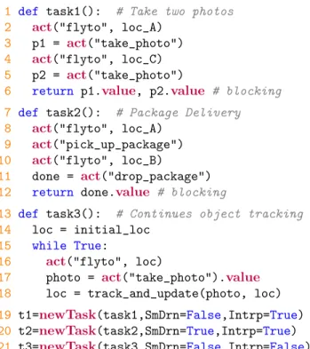
1 def task1(): # Take two photos

2 act("flyto", loc_A) 3 p1 = act("take_photo") 4 act("flyto", loc_C) 5 p2 = act("take_photo")

6 return p1.value, p2.value # blocking

7 def task2(): # Package Delivery

8 act("flyto", loc_A) 9 act("pick_up_package") 10 act("flyto", loc_B)

11 done = act("drop_package") 12 return done.value # blocking

13 def task3(): # Continues object tracking

14 loc = initial_loc

15 while True:

16 act("flyto", loc)

17 photo = act("take_photo").value

18 loc = track_and_update(photo, loc)

19 t1=newTask(task1,SmDrn=False,Intrp=True) 20 t2=newTask(task2,SmDrn=True,Intrp=True) 21 t3=newTask(task3,SmDrn=False,Intrp=False)

Figure 6: Example of different binding relationships. We show a code example in Figure 6 where there are three tasks with different binding relationships. We show a possible drone schedule in Figure 7.

Task 1. Task 1 has two actions - taking photos at location A and C. The actions can be executed on dif-ferent drones (SmDrn=False) and the time gap between two actions is not restricted (Intrp=True).

Task 2. Task 2 is a simple package delivery example. It requires the drone to pick up a package at location A and then drop it at location B. These two actions (pick up and drop) need to be executed on the same drone (SmDrn=True). However, the task can be interrupted (Intrp=True). After the package is picked up at location A, the drone can be scheduled to perform other actions

Task 1 Task 2 Task 3 Pick Up Package At Location A Drop Package At Location B Take Photo At Location A

Track Track Track Track Track

Take Photo At Location C Track Replace Battery Drone 2 Drone 1 SmDrn=False Intrp=True SmDrn=True Intrp=True SmDrn=False Intrp=False Interruptible Timeline

Figure 7: Fine-granularity multiplexing in BeeCluster before flying to location B.

Task 3. Task 3 is a continuous object tracking exam-ple where the drone is programmed to track a moving object. Each tracking step can be executed on different drones (SmDrn=False) but the time gap between two tracking steps should be minimized by the system to maintain high tracking success rate; thereby, the Intrp flag is set to False.

Through defining the binding relationship of tasks, developers can describe the resource requirements of their application precisely. This ability to specify bind-ing relationships makes inter-task multiplexbind-ing possible at a fine granularity – for example, one drone can carry out subtasks of several tasks when Intrp=True. This im-proves utilization of the drones, as shown in case study 4 in Section 5.2.1.

3.2

Application Forecasting

BeeCluster forecasts the application’s behavior through using the dynamic task graph (DTG) of the running ap-plication and by matching the current DTG with previ-ous historical DTGs (i.e., application profiling data).

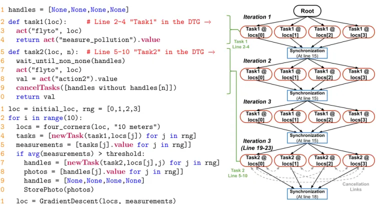
We show the source code of an example drone ap-plication in Figure 8 as well as its DTG. The applica-tion iteratively tracks the source of air polluapplica-tion using a gradient descent algorithm. At each iteration, if the air pollution is greater than a threshold, the application takes one photo at any one of the four locations involved in gradient computing step.

In this section, we use this example to describe the details of (1) the structure of DTG, (2) and how do we use the DTG to forecast the future behaviors of an application.

3.2.1

Dynamic Task Graph (DTG)

A dynamic task graph contains nodes and edges. Edges (directional) in a dynamic task graph represent the de-pendency relationship among nodes. Nodes have two types, task-nodes and synchronization-nodes.

A task-node corresponds to an instance of the task building block in BeeCluster API. For example, in Fig-ure 8, on line 14 (iteration 1), the application creates four tasks based on the function defined at line 3 with different input arguments. These four tasks correspond to the first four task-nodes in the dynamic task graph on the right side of Figure 8. Each task node contains the meta information for the task, including the first location to visit (if it exists), as well as the the prim-itives (act, newTask, cancelTasks) within the task and its duration.

A synchronization-node is used to represent the syn-chronization behavior of an application. Synchroniza-tion nodes are introduced by the use of the h.value API call. For example, on line 15, the execution is blocked until all the four tasks created in line 14 are completed. In the dynamic task graph, this synchronization behav-ior is represented as a synchronization node, i.e., the blue rectangle node in Figure 8.

The DTG doesn’t directly represent branches, e.g., the branch at line 16. When there is a branch, the dynamic task graph only contains the path that the ap-plication takes. For example, in the first two iterations, the sensing results don’t meet the branch condition at line 16. In this case, the DTG doesn’t contain the ex-ecution path of line 17-20 for the first two iterations because they don’t get executed.

BeeCluster’s runtime constructs the DTG of an run-ning application on the fly. The construction algorithm supports concurrent BeeCluster API calls from different application threads, allowing the developers to describe complicated application dependency logic.

3.2.2

Forecasting using DTGs

BeeCluster forecasts the future behaviour of a run-ning application through matching the most recent por-tion (sub-graph) of the current active DTG with histor-ical DTGs, including (1) the current active DTG with-out its frontier nodes (leaf-nodes) , (2) and the DTGs from past runs. Once a match is found, we can simply use what happened next in the historical DTGs as a forecast for what may happen next in the current appli-cation run.

Graph-Match and Forecast Algorithm. We call our forecasting algorithm GMF, for Graph Match and Forecast. The GMF algorithm contains two phases.

In the first phase, GMF searches for accurate sub-graph matches through an incremental matching pro-cedure. GMF starts with a sub-graph containing only one node (a frontier node) in the current DTG. This sub-graph is used as the target sub-graph for match-ing. Then, GMP finds all the one-node sub-graphs in the historical DTGs that match with this target sub-graph. All the matched one-node sub-graphs are con-sidered as candidate sub-graphs. Here, we say two task-nodes matched when they are from the same logic task but could have different input arguments.

After this, GMF starts to iteratively increase the depth of both the target graph and the candidate sub-graphs. At each iteration, GMF removes unmatched sub-graphs in the candidate sub-graphs from previous iteration. As the depth increases, the number of the can-didate sub-graphs decreases. This incremental matching procedure stops when the number of the candidate sub-graphs is below a threshold (10 in our implementation), or when the depth of the sub-graph exceeds a threshold (10 in our implementation).

In the second phase, GMF looks into the meta in-formation of each task-node and ranks all the matched candidate sub-graphs through a similarity metric. One meta information we used here is the first location a task visited, e.g, for a task that took a photo at location A, the first location it visited is location A.

Inspired by [46, 47], we use a rotation-and-translation-invariant distance, between the first locations of all the task-nodes in two matched sub-graphs as the similar-ity metric; given two sub-graphs, we apply a spatial transformation that only contains rotation and transi-tion to one of the sub-graph so that the total distance between the first locations of each node pairs is min-imized. This minimized distance is the rotation-and-translation-invariant distance between two sub-graphs. It is easy to extend this similarity metric to also con-sider the sensor readings, e.g., using cosine-similarity for image embeddings for image data captured at each task-node.

Finally, GMF outputs what happened next from the top-K, i.e., top-10, matched sub-graphs as a forecast. Here, we apply the spatial transformation to the pre-dicted task-nodes so that they have the correct loca-tions.

3.3

Extensible Optimization Heuristics

In this subsection, we first describe the BeeCluster’s scheduling model (Section 3.3.1), then we show how does BeeCluster support different optimizations as plu-gins in Section 3.3.2.

3.3.1

Scheduling Model

BeeCluster’s scheduling model uses instantaneous as-signment [23] of tasks to drones; in this model, the scheduler only needs to decide the next request each

1 handles = [None,None,None,None]

2 def task1(loc): # Line 2-4 "Task1" in the DTG −→ 3 act("flyto", loc)

4 return act("measure_pollution").value

5 def task2(loc, n): # Line 5-10 "Task2" in the DTG −→

6 wait_until_non_none(handles)

7 act("flyto", loc)

8 val = act("action2").value

9 cancelTasks([handles without handles[n]]) 10 return val

11 loc = initial_loc, rng = [0,1,2,3] 12 for i in range(10):

13 locs = four_corners(loc, "10 meters")

14 tasks = [newTask(task1,locs[j]) for j in rng]

15 measurements = [tasks[j].value for j in rng]]

16 if avg(measurements) > threshold:

17 handles = [newTask(task2,locs[j],j) for j in rng]

18 photos = [handles[j].value for j in rng]]

19 handles = [None,None,None,None]

20 StorePhoto(photos)

21 loc = GradientDescent(locs, measurements)

Task1 @ locs[0] Root Task1 @ locs[1] Task1 @ locs[2] Task1 @ locs[3] Task2 @ locs[0] Task2 @ locs[1] Task2 @ locs[2] Task2 @ locs[3] Synchronization (At line 18) Cancellation Links Synchronization (At line 15) Task1 @ locs[0] Task1 @ locs[1] Task1 @ locs[2] Task1 @ locs[3] Synchronization (At line 15) Task1 @ locs[0] Task1 @ locs[1] Task1 @ locs[2] Task1 @ locs[3] Synchronization (At line 15) Iteration 1 Iteration 2 Iteration 3 Iteration 3 (Line 19-23) Task 1 Line 2-4 Task 2 Line 5-10

Figure 8: Dynamic Task Graph (DTG) Example. drone needs to handle. The scheduler takes the current

states of the drones, the current visible requests, and the forecast requests as input, and outputs an instan-taneous assignment (a set of drone-to-request pairs). At high-level, the scheduler is triggered to reschedule drones when its input is changed. In our implementa-tion, we carefully choose when to reschedule to avoid system overhead; in particular, we try to batch changes to the input to eliminate frequent rescheduling.

Inside the scheduler, the scheduler employs simulated annealing [39] to search for the best instantaneous as-signment that maximizes the utility function. Here, the utility function is used to evaluate the goodness of the instantaneous assignment. In BeeCluster, this utility function is a linear combination of different sub-utility functions. Although the global goal of BeeCluster is to minimize the execution time of the application, we achieve that through optimizing the instantaneous as-signment at any point in time. Each sub-utility func-tion implements one optimizafunc-tion heuristic (we list a few below) that evaluate the goodness from one aspect. These sub-utility functions take the current configura-tion (both drones and requests) and an instantaneous assignment as input and outputs the utility (goodness) of the input instantaneous assignment. Here, we list a few sub-utility functions (optimization heuristics) as examples.

Closest Next Request Heuristic. This is the sim-plest greedy heuristic. The sub-utility function outputs the negative total estimated flying time of all

drone-to-request pairs in the instantaneous assignment.

Avoid Mutual Utility Heuristic. When there are two requests A and B in an application, and if A is done, B will be cancelled, if B is done, A will be cancelled. In this case, the system should not dispatch two drones to A and B at the same time. We implemented an opti-mization heuristic similar to the utility function in [12] to avoid having this happen. This heuristic relies on the forecast information provided by BeeCluster.

Avoid Zigzag Heuristic. We use this heuristic to avoid the worst case in Figures 1,2. This optimiza-tion heuristic also relies on the forecast informaoptimiza-tion pro-vided by BeeCluster. The sub-utility function com-putes the geometric center of all forecast and visible re-quests. Then, the sub-utility function causes the drones to visit the farthest request from this center by assign-ing a higher utility score to each drone-to-request pair when the request is far away from the geometry center. Speculative Execution Heuristic. When there are spare, idle drones in the system, this heuristic en-courages the spare drones to fly to their closest forecast requests. This heuristic is similar to the Closest Next Request Heuristic, but it operates only on forecast re-quests.

Fairness Heuristic. This sub-utility function out-puts the negative total waiting time of the involved re-quests in the drone-to-request pairs of the instantaneous assignment. This heuristic intends to give high priority to the requests that have long waiting time.

3.3.2

Optimization Heuristic Plugins and Automatic

Plugin Balancing

There exists many other optimization heuristics. As an extensible platform, BeeCluster provides an interface for optimization heuristic contributors so that they can easily add new optimization heuristics as plugins into the BeeCluster platform.

When there are multiple optimization heuristics avail-able in a system, it is hard to figure out what combina-tion (weights) of these heuristics can make a specific ap-plication run faster. In BeeCluster, we make the hyper-parameter tuning automatic. After several initial runs of an application, BeeCluster replays the executions of the application using the historical DTGs in a simulator and finds the linear weights for the different sub-utility functions (optimization heuristics) that minimizes exe-cution time using hyper-parameter search [17].

4.

IMPLEMENTATION

In this section, we show the implementation details of BeeCluster. We discuss the software in Section 4.1 and the hardware in Section 4.2.

4.1

BeeCluster Framework

BeeCluster Core API Layer

Hardware Abstraction Layer Python API

Wireless Layer

Drone Hub Simulator (Level 1)

Drone Endpoint

Drone-Specific

Driver Simulator (Level 2) Software/Hardware Boundary

DJI Drone Simulator (Level 3) Applications Centralized Onboard Python Golang C++

Figure 9: BeeCluster Framework

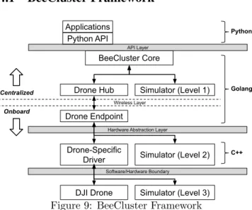
BeeCluster will be released as open-source. The im-plementation of the BeeCluster framework comprises ≈ 15K lines of code (LoC); 80.8% in Golang for the BeeCluster core system, 5.3% in python for the python wrapper of BeeCluster API, and 13.9% in C++ for the drone driver. We show a diagram of the BeeCluster component architecture in Figure 9.

Simulators. The implementation of BeeCluster in-volves three simulators. The level-1 simulator is used to conduct fast application replay for hyper-parameter search. The level-2 simulator is used to verify the cor-rectness of the system and the application before take-off. The level-3 simulator is DJI’s hardware simulator, which is used to verify the correctness of the drone driver

code. These simulators boost the development speed of BeeCluster and avoid potential failures in real-world ex-periments.

Drone-to-centralized controller communication protocol. In the implementation, the drone sends a heart-beat message to the centralized controller every 100 ms. The centralized controller encloses the action descriptions (if any) into the return message. Once the drone receives the return message, it performs the ac-tions enclosed in the return message and sends the result back to the centralized controller together with the next heart-beat message.

Collision avoidance and conflicts resolution (CACR). We implement a simple centralized first-come-first-serve CACR protocol in BeeCluster to avoid drone collisions and resolve conflicts. This CACR protocol is critical for real-world drone deployments.

4.2

Hardware Setup

mins flying time)

WiFi Antenna

Wide-Angle Camera

(a) (b)

Figure 10: Drone Hardware Used in Evaluation Similar to other drone orchestration system, BeeClus-ter is drone-agnostic. In our prototype, we use a cus-tom assembled drone platform as our drone back-end for evaluation. We show our drone platform in Fig-ure 10(a). Our drone platform is based on the DJI F450 drone frame [1]. We use DJI N3 flight controller [2] with a GPS antenna. The flight controller is connected to an on-board Raspberry Pi single-board computer [5]. Each drone is equipped with a 2dBm WiFi antenna, which enables communication (>150 meters) between the drone and the centralized controller. Each drone is also equipped with a wide angle camera for camera-based applications.

Drone profile. To make the simulator accurate, we profile the dynamic (acceleration rate, de-acceleration rate and drag coefficient) of our drones (Figure 10(b)). In our setup, the drone flies at 2 m/s when the target is within 20 meters, otherwise, the drone flies at 10 m/s.

5.

EVALUATION

In our evaluation, we seek to answer the following questions:

• What is the benefit of BeeCluster’s application-agnostic predictive optimization?

• What is the benefit of BeeCluster’s API? • What is the overhead of BeeCluster?

To address these questions, we evaluate BeeCluster with five case studies, consisting of four representative appli-cations and one proof-of-concept scenario consisting of three simple applications. We conduct most of our ex-periments with real drones and real environments. In addition, we use our level-2 simulator to conduct sim-ulated experiments that complement our real-world ex-periments.

5.1

Benefit from predictive Optimizations

5.1.1

Case Study 1: Road Mapping

Neural Network (CNN) Aerial

Image

Figure out the next location to visit

Drone in Mission

(a) Tracing Road Application Overview

(b) Real-World Experiments with One and Two Drones

One Drone

Two Drones Speculative Execution

First Iteration

First Iteration

Road Segmentation Aerial Image

Figure 11: Case Study 1: Mapping a Newly Constructed Road through Iterative Tracing

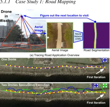
Automatically mapping new constructed roads is an important real-world task [10, 29, 20, 9, 28], e.g., for companies that maintain digital maps. For case study 1, we built a drone-based mapping application with the BeeCluster API where the drones can smartly map a newly constructed road through iterative road tracing. We show this application in Figure 11(a). The applica-tion begins at the start of the road. In each iteraapplica-tion, the application acquires a photo at the current location and computes the road position and direction through a neural network. Then, the application moves 6 meters along the road and starts the next iteration.

We evaluate this application on a newly constructed trail in a nearby park. We run the application for 25 iterations, which covers 144 meters of the trail. We show the drone trajectories in Figure 11(b). We highlight the positions of the trail at each iteration using a yellow circle.

Benefit: The application logic in this case study is an active sensing loop (see Section 2.1.1) with strong sequential dependencies; the i-th iteration depends on the execution result of the (i − 1)-st iteration.

(a) (b)

Figure 12: Benefits from Speculative Execution.

While the application is running, BeeCluster forecasts the locations where the application may need to visit in the future. When there are spare drones in the system, BeeCluster dispatches the spare drones to the forecast locations. This speculative execution strategy overlaps the sensing time and flying time of the active sensing loop, reducing the total execution time of the applica-tion. To show this, we added a second drone. We show drone trajectories in Figure 11(b). In the two-drone scenario, we can clearly see that the two drones alterna-tively fly over each other. Here, the curvy traces are the result of our collision avoidance and conflict resolution protocol.

We repeat the experiments three times for both the one-drone scenario and two-drone scenario. As shown in Figure 12(a), BeeCluster’s speculative execution strat-egy improves the sensing task runtime by 21.3%. Here, the baseline approach does not support speculative ex-ecution, instead, it only executes the program line by line. In fact, the benefit of the speculative execution heavily depends on the ratio of sensing time to flying time. We simulated different sensing time to flying time ratios for the tracing road application in a simulator. As shown in Figure 12(b), we find speculative execu-tion performs the best when the ratio of sensing time to flying time is close to 1.5, which achieves up to 50% performance improvement.

In this case study, we don’t use historical DTGs; the forecast is only based on the early portion of the active DTG, e.g., the first few iterations. We find this setup is sufficient because the application is predictable and the speculative execution does not require very accurate predictions to overlap the flying time and sensing time.

5.1.2

Case Study 2: Wifi Coverage Map

In case study 2, we built an application with the BeeCluster API to create a WiFi coverage map of an open area. Our application adapts an efficient and pop-ular information gathering algorithm based on Gaussian Processes [34].The algorithm first divides the region of interest into an equal sized grid (i.e., 5 meters by 5 meters). Then, the algorithm issues tasks (using the newTask primitive) to request a WiFi signal strength measurement from all grid cells. When the WiFi signal strength is measured at a grid, the algorithm updates

(a) Reactive (Baseline) Flight TIme: 270 seconds

(b) Predictive (BeeCluster) Flight TIme: 228 seconds

(c) Wifi Signal Coverage Map (Gaussian Process) Start End End Start Wifi Hotspot dBm

Figure 13: Case Study 2: Mapping Wifi Signal Coverage through a Gaussian Process

the Gaussian Process model (which models the WiFi signal strength field) and updates the uncertainty esti-mate on all other grids. If the uncertainty estimation of a grid falls below a threshold, the measurement request in that grid is cancelled (using the cancelTask primi-tive). The algorithm stops when all the grid cells are measured or have satisfied the uncertainty threshold.

We evaluate this application in a 50 meter by 70 meter open area. In Figure 13(a,b), we show the center of each 5 meter by 5 meter grid cell in green and highlight the visited grid cells in yellow. We show the estimated WiFi coverage map in Figure 13(c).

Benefit: In this case study, BeeCluster forecasts the task cancellation behavior of the application. Here, we use one additional historical DTG from a previous run in the simulator. We find the best weights of different optimization heuristics through replaying this DTG in a simulator. We find this simulated DTG can be trans-ferred to our real-world environment. Then, inside the scheduler, the Avoid Mutual Utility Heuristic (Section 3.4.1) uses the forecast information to encourage drones to visit the grids that maximize the expected informa-tion gain. We can clearly see the effect of this predictive optimization heuristic in Figure 13(a,b). In the baseline (only with reactive optimization), the drone visits grids on the boundary of the region. In contrast, BeeCluster’s predictive optimization strategy causes drones to visit grids that are at least one grid away from the bound-ary. This is because once a grid is visited, its neigh-boring grids will be cancelled with a high probability. Note that BeeCluster captures this insight without re-quiring explicit input from the application, simply using the Avoid Mutual Utility heuristic.

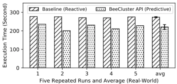
We repeat the experiments 5 times with real drones and real environments. As shown in Figure 14, BeeClus-ter’s predictive optimization yields an 23.9% average runtime improvement in this scenario.

5.1.3

Case Study 3: Wifi Hotspot Localization

1

2

3

4

5

avg

Five Repeated Runs and Average (Real-World)

0

100

200

300

Execution Time (Second)

Baseline (Reactive) BeeCluster API (Predictive)

Figure 14: BeeCluster enables Application Agnostic pre-dictive Optimization, reducing the execution time by 23.9% on average over five runs in case study 2

statement from lines 16 to 20.

We evaluate this application with real drones and real environments. In the evaluation, we set the initial lo-cation of the algorithm to be 60 meters away from the hotspot and then ran the algorithm for ten iterations. In each iteration, the current location moves 5 meters toward the direction of the gradient. We show an ex-ample trajectory in Figure 15(a).

(a) Experiment Environment (b) Result

WiFi Hotspot Start

Local-Optimal But Not Global-Optimal

Global Optimal (After Collecting Enough Application Information)

Figure 15: Case Study 3: WiFi Hotspot Localization Benefit: In this case study, BeeCluster can forecast the new tasks generated by the applications. As the four measurements in each iteration don’t have an order, the baseline solution (reactive) may not always pick up the best order (clockwise or counter-clockwise) in which to perform the measurements. In contrast, BeeClus-ter leverages forecasting information to always pick the best order. We repeat the experiments 5 times. We show the average execution time of the last 5 iterations in Figure 15(b). BeeCluster’s predictive optimization improves the performance by 11.6% against reactive op-timization.

In this case study, we don’t use historical DTGs; the forecast is only based on the early portion of the ac-tive DTG, e.g., the first few iterations. As shown in Figure 15(a), the drone didn’t always follow the global optimal route in the first few iterations. Later on, once the system collected enough application profiling data (DTG), the drone started to always follow the global optimal route.

5.2

Benefit from BeeCluster API

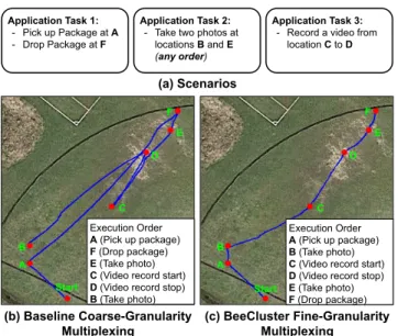
Start A B C D E F Start A B C D E F Execution Order A (Pick up package) F (Drop package) E (Take photo) C (Video record start) D (Video record stop) B (Take photo)

Execution Order

A (Pick up package) B (Take photo) C (Video record start) D (Video record stop) E (Take photo) F (Drop package) (b) Baseline Coarse-Granularity Multiplexing (c) BeeCluster Fine-Granularity Multiplexing (a) Scenarios Application Task 1: - Pick up Package at A - Drop Package at F Application Task 2:

- Take two photos at locations B and E

(any order)

Application Task 3: - Record a video from

location C to D

Figure 16: Case Study 4 Fine Granularity Multiplexing In this case study, we built a proof-of-concept scenario to demonstrate the benefit of BeeCluster’s precise bind-ing relationships. We create three fake application tasks (Figure 16(a)) with different binding relationships. The first application task mimics the package delivery task. It needs to pick up a package at A and drop it at F. The task requires the same drone to do the pickup and dropoff but the task is interruptible. The second ap-plication task takes two photos at two locations B and E. The two photos can be taken in any order (imple-mented with newTask primitive). The third application task record a video from location C to D. The task re-quires the same drone to record and the task is not interruptible.

In the evaluation, we submit these three application tasks to the drone orchestration system (with one drone). We fix the locations A and F and randomly generate the other four locations to create 10 different random sce-narios. In the baseline orchestration system, we disable the precise binding definition in application task 1 but keep the application tasks 2 and 3 the same. In this case, once the application task 1 starts, the drone is occupied until the application task 1 is completed.

Benefit: We repeat the experiment 10 times with real drones. We show the quantitative result in Fig-ure 17. BeeCluster surpasses the baseline by 19.1% in terms of execution time. This improvement comes from fine-granularity multiplexing; as shown in Figure 16(c), BeeCluster can multiplex application task 1 with other tasks; once the drone picks up the package at location A, it doesn’t need to send the package to location F immediately, instead, the drone can still conduct other tasks along the way to location F.

5.2.2

Case Study 5: Continuous Object Tracking

1

2

3

4

5

6

7

8

9 10 avg

Scenarios

0

20

40

60

80

100

Execution Time (Second)

Baseline (Coarse-Granularity Multiplexing)

BeeCluster API (Fine-Granularity Multiplexing)

Figure 17: BeeCluster API enables fine granularity mul-tiplexing, reducing the execution time by 19.1% on av-erage over ten runs in case study 4

Target to Track

(b) View from Drone

(a) Trajectories Hand-Off 1 Hand-Off 2 Hand-Off 3 Hand-Off 4 Hand-Off 5 Start End Battery Replace Zone Drone 2 Drone 1 Target Trace (c) Hand-Off Overhead

Figure 18: Case Study 5: Continuous object tracking beyond a single drone’s battery life.

For case study 5, we built an application to continu-ously track a person. The duration of the tacking task is longer than the battery-time of a single drone. We use this case study to demonstrate the effect of the non-same drone but uninterruptible binding relation-ship (see Section 3.2.2). The application logic is similar to line 13-18 in Figure 7.

We use two real drones in this experiment. We arti-ficially limit the flying time of each drone to be only 60 seconds. After the battery is used up, the drone needs to fly back home to simulate recharging its battery (in reality the drones have about 30 minutes of battery life, so actual battery replacement wasn’t necessary). In the experiment, we track a moving person for 5 minutes (with 5 drone hand-offs). We show the trajectories of the two drones in Figure 18(b).

Benefit: We demonstrate that BeeCluster can sup-port continuous operation beyond a single drone’s bat-tery time without any additional code - but with a small overhead; we show the average execution times of each regular iteration and each hand-off iteration in Figure 18(c). Here, the hand-off iterations are the iter-ations where the hand-off happened.

5.3

BeeCluster Overhead

Next, to study the overhead of the BeeCluster frame-work, we measured the execution time of each

compo-0% 20% 40% 60% 80% 100% CaseStudy 5 CaseStudy 3 CaseStudy 2 CaseStudy 1 Application

Flying DriverTransmission (payload) Transmission (sync)System Overhead

Figure 19: Execution Time Breakdown

nent for case studies 1,2,3, and 5. Case study 4 is a proof-of-concept scenario, so we don’t consider it in this measurement. In this measurement, we use only one drone and repeat each application three times. We show the execution time breakdown of all our the four appli-cations in Figure 19.

There are six parts in the execution time breakdown. Application time is the time spent within the applica-tion (python), including the sleep funcapplica-tion call. Flying time is the amount of time when the drone is flying to-ward target. Driver time is the amount of time spent inside the driver, e.g., taking a photo may take 100-200 ms. Transmission time consists of two parts: transmis-sion (payload) time is the time spent sending the data between the drone and the centralized controller; trans-mission (sync) time is the delay introduced by the fixed rate (synchronized) drone-to-centralized controller com-munication protocol (See Section 4.1). On average, this protocol introduces a 150 ms (100 ms + 50 ms) delay for each action.

The overhead of BeeCluster, which includes dynamic task graph construction, application forecasting, and scheduling, is the difference between the five compo-nents described above and the total wall-clock execu-tion time1_{. The average system overhead of the four} applications is 2.34%, which we believe is acceptable.

Scalability For completeness, we show the schedul-ing time and the forecast time with different numbers of drones and historical DTGs in Figure 20. Here, the results are from case study 2 for scheduling time, and from case study 3 for forecast time because these two ap-plications have the highest overhead in scheduling and forecast, respectively. We use level-2 simulator to mea-sure these overhead.

1_{This is because we only use one drone.}

Figure 20: Scheduling Time and Forecasting Time

6.

RELATED WORK

Work related to drone orchestration has been done in different fields, including computer systems, robotics, and operations research. Figure 21 illustrates how BeeClus-ter is different from existing work.

Reliability Isolation Optimization Complexity Platform Flexibility Single-purpose Applications Existing Drone Orchestration Systems BeeCluster Low-level Control Other Orthogonal Dimensions General-Purpose Platform Single-Purpose Platform Static Optimization Reactive Optimization Predictive Optimization Domain-Specific Platform

Figure 21: Positioning of BeeCluster vs Related Work In contrast to prior drone orchestration systems such as AnDrone [40], Voltron [30], and UAV-as-a-service [25, 26, 48], our main contribution is developing a predictive optimization strategy, in contrast the non-predictive na-ture of prior work. In addition, we designed a novel general-purpose programming API that allows develop-ers to describe the logic of a wide range of drone ap-plications in a precise way. This new API enables our predictive optimizations.

In contrast to single-purpose drone applications [35, 36, 8, 15, 22, 41], BeeCluster provides predictive op-timization in a transparent way. Unlike many single-purpose applications or algorithms, which, if they are predictive, require application developers to provide the information needed to make predictions, BeeCluster in-fers the necessary information from the program execu-tion and profiling data.

There are other important aspects in a drone orches-tration system that have been studied, including low-level drone control [11], reliable communication proto-cols [21, 13], and isolation [40]. This work is comple-mentry and orthogonal to BeeCluster.

7.

CONCLUSION

In this work, we described a new drone orchestration system, BeeCluster. BeeCluster is able to take into ac-count the future sensing tasks that applications will exe-cute when making scheduling decisions. This is achieved

through a novel programming API that allows develop-ers to describe the logic of a wide range of drone ap-plications in a precise and compact way, as well as an extensible rule-based forecasting approach. We demon-strate the effectiveness BeeCluster through a evalua-tion over five real-world case studies with real drones in outdoor environments, demonstrating speedups ranging from 11.6% to 23.9%.

8.

REFERENCES

[1] Dji f450 drone frame.

https://www.dji.com/flame-wheel-arf. [2] Dji n3 flight controller. https://www.dji.com/n3. [3] Dronedeploy. https://www.dronedeploy.com. [4] Pix4dcapture. https:

//www.pix4d.com/product/pix4dcapture. [5] Raspberry pi. https://www.raspberrypi.org/. [6] Adams, S. M., and Friedland, C. J. A survey

of unmanned aerial vehicle (uav) usage for imagery collection in disaster research and management. In 9th International Workshop on Remote Sensing for Disaster Response (2011), vol. 8.

[7] Ad˜ao, T., Hruˇska, J., P´adua, L., Bessa, J., Peres, E., Morais, R., and Sousa, J. Hyperspectral imaging: A review on uav-based sensors, data processing and applications for agriculture and forestry. Remote Sensing 9, 11 (2017), 1110.

[8] Alvear, O., Zema, N. R., Natalizio, E., and Calafate, C. T. Using uav-based systems to monitor air pollution in areas with poor

accessibility. Journal of Advanced Transportation 2017 (2017).

[9] Bastani, F., He, S., Abbar, S., Alizadeh, M., Balakrishnan, H., Chawla, S., and Madden, S. Machine-assisted map editing. In Proceedings of the 26th ACM SIGSPATIAL International Conference on Advances in Geographic Information Systems (2018), ACM, pp. 23–32.

[10] Bastani, F., He, S., Abbar, S., Alizadeh, M., Balakrishnan, H., Chawla, S., Madden, S., and DeWitt, D. Roadtracer: Automatic extraction of road networks from aerial images. In Proceedings of the IEEE Conference on Computer Vision and Pattern Recognition (2018),

pp. 4720–4728.

[11] Bregu, E., Casamassima, N., Cantoni, D., Mottola, L., and Whitehouse, K. Reactive control of autonomous drones. In Proceedings of the 14th Annual International Conference on Mobile Systems, Applications, and Services (2016), MobiSys ’16.

[12] Burgard, W., Moors, M., Stachniss, C., and Schneider, F. E. Coordinated multi-robot

exploration. IEEE Transactions on robotics 21, 3 (2005), 376–386.

[13] Chlestil, C., Leitgeb, E., Schmitt, N. P., Muhammad, S. S., Zettl, K., and Rehm, W. Reliable optical wireless links within uav swarms. In 2006 international conference on transparent optical networks (2006), vol. 4, IEEE, pp. 39–42. [14] Doherty, P., and Rudol, P. A uav search and

rescue scenario with human body detection and geolocalization. In Australasian Joint Conference on Artificial Intelligence (2007), Springer, pp. 1–13.

[15] Dorling, K., Heinrichs, J., Messier, G. G., and Magierowski, S. Vehicle routing problems for drone delivery. IEEE Transactions on Systems, Man, and Cybernetics: Systems 47, 1 (2016), 70–85.

[16] Eschmann, C., Kuo, C.-M., Kuo, C.-H., and Boller, C. Unmanned aircraft systems for remote building inspection and monitoring. In Proceedings of the 6th European Workshop on Structural Health Monitoring, Dresden, Germany (2012), vol. 36.

[17] Feurer, M., and Hutter, F. Hyperparameter Optimization. Springer International Publishing, Cham, 2019, pp. 3–33.

[18] Floreano, D., and Wood, R. J. Science, technology and the future of small autonomous drones. Nature 521, 7553 (2015), 460–466. [19] Ham, Y., Han, K. K., Lin, J. J., and

Golparvar-Fard, M. Visual monitoring of civil infrastructure systems via camera-equipped unmanned aerial vehicles (uavs): a review of related works. Visualization in Engineering 4, 1 (2016), 1.

[20] He, S., Bastani, F., Abbar, S., Alizadeh, M., Balakrishnan, H., Chawla, S., and Madden, S. RoadRunner: Improving the precision of road network inference from gps trajectories. In ACM SIGSPATIAL (2018). [21] Ho, D.-T., and Shimamoto, S. Highly reliable

communication protocol for wsn-uav system employing tdma and pfs scheme. In 2011 IEEE Globecom Workshops (Gc Wkshps) (2011), IEEE, pp. 1320–1324.

[22] Julian, K. D., and Kochenderfer, M. J. Distributed wildfire surveillance with autonomous aircraft using deep reinforcement learning. Journal of Guidance, Control, and Dynamics (2019), 1–11. [23] Korsah, G. A., Stentz, A., and Dias, M. B.

A comprehensive taxonomy for multi-robot task allocation. The International Journal of Robotics Research 32, 12 (2013), 1495–1512.

[24] Lin, Y., Hyyppa, J., and Jaakkola, A. Mini-uav-borne lidar for fine-scale mapping. IEEE

Geoscience and Remote Sensing Letters 8, 3 (2010), 426–430.

[25] Mahmoud, S., Mohamed, N., and

Al-Jaroodi, J. Integrating uavs into the cloud using the concept of the web of things. Journal of Robotics 2015 (2015), 10.

[26] Mahmoud, S. Y. M., and Mohamed, N. Toward a cloud platform for uav resources and services. In 2015 IEEE Fourth Symposium on Network Cloud Computing and Applications (NCCA) (2015), IEEE, pp. 23–30.

[27] M´ath´e, K., and Bu¸soniu, L. Vision and control for uavs: A survey of general methods and of inexpensive platforms for infrastructure

inspection. Sensors 15, 7 (2015), 14887–14916. [28] M´attyus, G., Luo, W., and Urtasun, R.

Deeproadmapper: Extracting road topology from aerial images. In Proceedings of the IEEE

International Conference on Computer Vision (2017), pp. 3438–3446.

[29] M´attyus, G., Wang, S., Fidler, S., and Urtasun, R. Hd maps: Fine-grained road segmentation by parsing ground and aerial images. In Proceedings of the IEEE Conference on Computer Vision and Pattern Recognition (2016), pp. 3611–3619.

[30] Mottola, L., Moretta, M., Whitehouse, K., and Ghezzi, C. Team-level programming of drone sensor networks. In Proceedings of the 12th ACM Conference on Embedded Network Sensor Systems (2014), ACM, pp. 177–190.

[31] Nex, F., and Remondino, F. Uav for 3d mapping applications: a review. Applied geomatics 6, 1 (2014), 1–15.

[32] Puri, A. A survey of unmanned aerial vehicles (uav) for traffic surveillance. Department of computer science and engineering, University of South Florida (2005), 1–29.

[33] Quaritsch, M., Kruggl, K.,

Wischounig-Strucl, D., Bhattacharya, S., Shah, M., and Rinner, B. Networked uavs as aerial sensor network for disaster management applications. e & i Elektrotechnik und

Informationstechnik 127, 3 (2010), 56–63. [34] Rasmussen, C. E. Gaussian processes in

machine learning. In Summer School on Machine Learning (2003), Springer.

[35] Rossi, M., Brunelli, D., Adami, A.,

Lorenzelli, L., Menna, F., and Remondino, F. Gas-drone: Portable gas sensing system on uavs for gas leakage localization. In SENSORS, 2014 IEEE (2014), IEEE, pp. 1431–1434. [36] Ruiz, A. V., Angermann, M., Wieser, I.,

Frassl, M., and Mueller, J. Efficient multi-agent exploration with gaussian processes.

In Australasian Conference on Robotics and Automation (ACRA) (2014).

[37] Saari, H., Pellikka, I., Pesonen, L., Tuominen, S., Heikkil¨a, J., Holmlund, C., M¨akynen, J., Ojala, K., and Antila, T. Unmanned aerial vehicle (uav) operated spectral camera system for forest and agriculture

applications. In Remote Sensing for Agriculture, Ecosystems, and Hydrology XIII (2011), vol. 8174, International Society for Optics and Photonics, p. 81740H.

[38] Smith, J. E. A study of branch prediction strategies. In Proceedings of the 8th annual symposium on Computer Architecture (1981), IEEE Computer Society Press, pp. 135–148. [39] Van Laarhoven, P. J., and Aarts, E. H.

Simulated annealing. In Simulated annealing: Theory and applications. Springer, 1987, pp. 7–15. [40] Van’t Hof, A., and Nieh, J. Androne: Virtual

drone computing in the cloud. In Proceedings of the Fourteenth EuroSys Conference 2019 (2019), ACM, p. 6.

[41] Vasisht, D., Kapetanovic, Z., Won, J.-h., Jin, X., Chandra, R., Kapoor, A., Sinha, S. N., Sudarshan, M., and Stratman, S. Farmbeats: An iot platform for data-driven agriculture. In Proceedings of the 14th USENIX Conference on Networked Systems Design and Implementation (2017).

[42] Villa, T., Gonzalez, F., Miljievic, B., Ristovski, Z., and Morawska, L. An overview of small unmanned aerial vehicles for air quality measurements: Present applications and future prospectives. Sensors 16, 7 (2016), 1072. [43] Villa, T., Salimi, F., Morton, K.,

Morawska, L., and Gonzalez, F.

Development and validation of a uav based system for air pollution measurements. Sensors 16, 12 (2016), 2202.

[44] Viseras, A., Shutin, D., and Merino, L. Online information gathering using

sampling-based planners and gps: an information theoretic approach. In 2017 IEEE/RSJ

International Conference on Intelligent Robots and Systems (IROS) (2017), IEEE, pp. 123–130. [45] Viseras, A., Wiedemann, T., Manss, C.,

Magel, L., Mueller, J., Shutin, D., and Merino, L. Decentralized multi-agent exploration with online-learning of gaussian processes. In 2016 IEEE International Conference on Robotics and Automation (ICRA) (2016), IEEE, pp. 4222–4229. [46] Vlachos, M., Gunopulos, D., and Das, G.

Rotation invariant distance measures for trajectories. In Proceedings of the tenth ACM SIGKDD international conference on Knowledge

discovery and data mining (2004), ACM, pp. 707–712.

[47] Werman, M., and Weinshall, D. Similarity and affine invariant distances between 2d point sets. IEEE Transactions on Pattern Analysis and Machine Intelligence 17, 8 (1995), 810–814. [48] Yapp, J., Seker, R., and Babiceanu, R. Uav

as a service: Enabling on-demand access and on-the-fly re-tasking of multi-tenant uavs using cloud services. In 2016 IEEE/AIAA 35th Digital Avionics Systems Conference (DASC) (2016), IEEE, pp. 1–8.

[49] Yungaicela-Naula, N. M., Zhang, Y., Garza-Casta˜non, L. E., and Minchala, L. I. Uav-based air pollutant source localization using gradient and probabilistic methods. In 2018 International Conference on Unmanned Aircraft Systems (ICUAS) (2018), IEEE, pp. 702–707.