Patient specific identification of the cardiac driver function in a cardiovascular system model.
Texte intégral
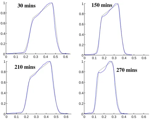
Figure

Documents relatifs
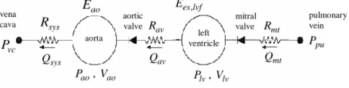
In order to be able to analyse data from different autonomic tests, two configurations, showing different levels of detail of the vascular system, have been proposed: a
A “relevant cohort” could comprise patients with stroke/transient ischae- mic attack (TIA), or suspected cognitive impairment or de- mentia, or healthy subjects, from a hospital
Figure 4: Comparison of the 110 m wind direction (a) and speed (b) observed and forecasted, represented by the probability density function (color scale). The densities are
The CoRoT (Convection Rotation and Planetary Transits) satellite, launched in December 2006, has now measured oscillations and the stellar granulation signature in three main
Outre cet effet érythropoïétique, l’EPO module la réponse ventilatoire à l’hypoxie (RVH) par une action directe sur la commande centrale respiratoire (CCR) et les
Features to be added to new systems include thruster allocation for azimuthing thrusters; digital motion controller hardware; improved wave filtering; optimal control design;
We will show (in the “ Erroneous conclusions about PEGS amplitudes ” section) that stacking the same data as K19, but after instrument response correction fol- lowing
