HAL Id: cea-02339415
https://hal-cea.archives-ouvertes.fr/cea-02339415
Submitted on 26 Mar 2020HAL is a multi-disciplinary open access archive for the deposit and dissemination of sci-entific research documents, whether they are pub-lished or not. The documents may come from teaching and research institutions in France or abroad, or from public or private research centers.
L’archive ouverte pluridisciplinaire HAL, est destinée au dépôt et à la diffusion de documents scientifiques de niveau recherche, publiés ou non, émanant des établissements d’enseignement et de recherche français ou étrangers, des laboratoires publics ou privés.
Local-scale valley wind retrieval using an artificial neural
network applied to routine weather observations
Florian Dupuy, Gert-Jan Duine, Pierre Durand, Thierry Hedde, Pierre
Roubin, Eric Pardyjak
To cite this version:
Florian Dupuy, Gert-Jan Duine, Pierre Durand, Thierry Hedde, Pierre Roubin, et al.. Local-scale valley wind retrieval using an artificial neural network applied to routine weather observations. Journal of Applied Meteorology and Climatology, American Meteorological Society, 2018, 58 (5), pp.1007-1022. �10.1175/JAMC-D-18-0175.1�. �cea-02339415�
Valley-winds at the local scale: A downscaling method based on artificial neural network applied to routine weather forecasting
Florian Dupuy(1,2), Gert-Jan Duine(3), Pierre Durand(1), Thierry Hedde(2), Pierre Roubin(2) (1) Laboratoire d’Aérologie, Université de Toulouse, CNRS, UPS, Toulouse
(2) Laboratoire de Modélisation des Transferts dans l’Environnement, CEA Cadarache, Saint-Paul-lès-Durance, France
(3) University of Virginia (à voir avec Gert-jan)
Abstract
In regions of complex topography, the local flows (i.e. at the sub-kilometer scale) are difficult to forecast on a routine basis because of the too coarse resolution of operational models. The worst performance is obtained for stable stratifications, which are yet the most problematic situations regarding the accumulation of pollutants. In the SE of France, the Cadarache site features such a complex topography. Furthermore, the region is also characterized by a high occurrence of clear skies often leading to stable boundary layers during nighttime periods.
The Weather Research and Forecasting (WRF) model is run daily to forecast the weather in this region with a horizontal resolution of 3 km. These simulations cannot resolve all the details of the topography and particularly the narrow Cadarache valley, where local wind patterns are therefore not accessible. However, other variables, less dependent on the sub-grid topography, are satisfactorily forecasted and thus used as inputs in an artificial neural network (ANN) used to downscale wind patterns in the valley.
Using the vertical gradient of temperature and the horizontal wind as ANN input parameters, this method allows improving the forecast of the low level wind (direction and speed) at one spot in the Cadarache valley. The training and qualification of the ANN is based on observations of the wind in the valley during an entire year. The Directional Accuracy (DACC), which represents the fraction of wind directions that do not depart from the observations by more than 45°, then jumps from 0.56 for WRF simulations to 0.75 for ANN output, and the Proportion Correct (PC), which represents the fraction of data that are well classified regarding different ranges of wind direction, increases from 0.53 for WRF to 0.74 for the ANN.
This study demonstrates the potential of the ANN technique used as a downscaling tool to forecast weather conditions at the local scale when numerical modeling is done at a too coarse resolution to represent the effect of the local topography.
1. Introduction
Low level winds must be well described when studying the atmospheric dispersion. Stable conditions are among the most impacting because they trap the pollutants near the surface. Moreover, over complex topography, stable conditions can generate gravity/density flows along the slopes ( (Muñoz, et al., 2013); (Largeron, 2010); (Duine, 2017); (Simpson, 1994)), and cold pools ( (Burns, et al., 2014); (Lareau, et al., 2013); (Price, et al., 2011); (Clements, et al., 2003)), thereby modifying the atmospheric dispersion. By different ways, the topography can generate terrain-induced phenomena near the surface (Chow, et al., 2013) impacting the low level variables, and especially winds when channeling effects dominate downward momentum transport (Whiteman, et al., 1993).
Several experiments have been conducted to study density driven, valley and slope flows and/or cold pooling, like e.g. the VTMX- (Doran et al. 2002), COLPEX- (Price, et al., 2011),METCRAX- (Whiteman et al. 2008), Materhorn- (Fernando et al., 2015) or ASCOT-campaign (Clements et al. 1989). In the recent
past years, a steep alpine valley was documented during the Passy project (Paci and Staquet 2016), and the KASCADE (Katabatic winds and Stability over CAdarache for Dispersion of Effluents) experiment (Duine et al., 2017) has been conducted in winter 2013 in the Cadarache region (SE of France) which features a complex topography.
In numerical weather predictions, the representation of these local phenomena depends on the representation of the topography which is itself related to the horizontal grid resolution and the associated modeling limitations. The choice of coarse resolutions is mostly determined by the computational cost that increases with resolution. Another limitation for the horizontal resolution is the range of validity of parametrizations such as the 1D turbulence schemes which do not allow resolutions finer than around one kilometer. For finer resolutions, the larger turbulent eddies become explicitly calculated. However, it is accepted that a large eddy simulation (LES) is satisfactory once at least 80% of the total kinetic energy is resolved (Pope, 2001). This introduces a threshold for the horizontal resolution. Thus, Wyngaard, (2004) introduced the “terra incognita” to define the range of horizontal resolutions (approximately 1 km to 100 m) for which it is possible neither to completely parameterize the turbulence nor to explicitly represent enough of the turbulence spectrum to run a proper LES. For these reasons, routine forecasting simulations generally use (at best) kilometric horizontal resolutions.
In Cadarache, one of the sites of the "Commissariat à l’Énergie Atomique et aux Énergies Alternatives" (CEA, the French nuclear agency), routine forecasts are run using the WRF model
(Skamarock, et al., 2008) at a 3 km horizontal resolution. Such coarse resolutions allow neither to represent the very complex topography of the Cadarache region, nor their associated local winds. However, for sanitary purposes, there is a need for operational forecasts of local winds on and around industrial sites, and more generally over any region with such a complex topography.
To fill this gap in the operational forecasts, Duine et al., (2016) have developed a method to nowcast the occurrence of down-valley winds, occurring under stable conditions in a small valley at Cadarache, as they were observed during the KASCADE campaign (Duine et al., 2017). They found that, among the permanent measurements available, a vertical temperature difference is a good indicator of the presence of the down-valley wind. This method represents a first step of downscaling for the knowledge of a local wind, however, since it is based on observations, it is restricted to the nowcasting and cannot improve the forecast of these local winds.
Another nowcasting tool frequently used in atmospheric studies is the Artificial Neural Network (ANN). Gardner and Dorling (1998) give an overview of the scope of their utilization in atmospheric studies. An ANN is a statistical tool which allows correlating some variables between each other, even being blind about the physical link between the variables. Its principle is to search the better relation between some variables (inputs, always available) to calculate an output that is the closest to an observation (target, temporarily available). Up to now, the common utilization of ANN has been to link observed variables (for input and target), whereas there were no studies linking simulated variables with observations. It has been successfully used to estimate the wind speed (Philippopoulos and Deligiorgi, 2012; Cadenas and Rivera, 2009; More and Deo, 2003), with better performances than more traditional statistical methods. Delon et al. (2007) used this technique to determine nitrogen oxide soil emission from environmental variables. Coulibaly et al. (2005) used a neural network to downscale temperature and precipitation observations, whereas Liu and Coulibaly (2011)
applied the same technique to improve hydrologic forecasting on a weekly time scale. ANN were also used for short term forecasting (one to a few hours) of the wind speed (Liu et al. (2015); Hu et al. (2016)).
The aim of this study is to build an ANN, using simulated variables as inputs (from the operational WRF simulations outputs) and observations as targets (temporary observations used to train the ANN). In order to go beyond the study of Duine et al. (2016), the betterment of the combinational use of an ANN and numerical simulations is to downscale mesoscale simulations to forecast a local wind. The paper is organized as follows: In the first section, the site of the study and the data used are described. The next section is dedicated to the presentation of the numerical weather predictions with the WRF model, and their evaluation against observations. Then, the third part introduces the ANNs, their utilization jointly with the WRF output and the results they brought. Finally, these results are discussed in the last part.
2. Site and observations 2.1 Description of the site
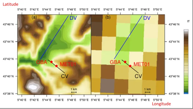
The study is focused on the CEA Cadarache Center located in south-eastern France, 50 km north of the Mediterranean Sea and near the Alps Mountains, in a pre-alps region featuring a lot of small valleys and mounts (Figure 1a). Especially, Cadarache is situated at the junction of two valleys: the middle Durance valley (DV), oriented north-north-east to south-south-west (approximately 67 km long, 200 m deep, 5 km wide with a mean slope of 0.2°) and the smaller Cadarache valley (CV) oriented south-east to north-west (approximately 6 km long, 100 m deep, 1 to 2 km wide with a mean slope of 1.2°, Duine et al., (2017)).
Typical regional meteorological phenomena occurring in the region are sea breeze (Cros et al., 2004) and Mistral (Bastin et al., 2005) which is a regional wind caused by channeling along the Alps and Massif Central mountains (from the north to the south). Precipitation events are usually brought by south-east winds. The region is also often subject to heavy precipitation events (Berthou et al., 2016), especially during the fall. Furthermore, the region is characterized by a high occurrence of clear skies leading to frequent stable conditions during nighttime and producing thermally-driven down-valley winds. These conditions were investigated during the KASCADE experiment (from 13th December 2012 to 18th March 2013, Duine et al., 2017). The main goal of this experiment was to observe the evolution of characteristic winds on the Cadarache site and especially during stable conditions. During daytime, the
typically westerly wind results from a synoptic forcing or a sea breeze. After sunset, when the synoptic forcing is low enough, stable conditions can occur, leading to the formation of a down-valley wind in the Cadarache valley. Its thickness is about 50 m with a maximum speed at 25-30 m. The stability quickly collapses after sunrise, and the westerly wind comes back. Above this Cadarache down-valley wind, and under the same conditions of formation, another wind develops from around 200 m above ground level and up to about 600 m, going down the Durance valley.
Figure 1: (a) Topography of the region of Cadarache as represented in WRF with a 111 m horizontal resolution. The blue line represents the Durance valley (DV), the black line represents the Cadarache valley (CV) and the red dots represent the locations of the meteorological stations MET01 and GBA. (b) Topography of the same area as represented in WRF simulations at 3 km of horizontal resolution.
2.2 Available observations
The observations used in this study are twofold: time-limited and permanent. Inside the Cadarache valley at the MET01 station, numerous observations were made along the vertical during the 3-month period of the KASCADE experiment, and a meteorological station was operated at 2 m in the same place from July 01, 2014 to February 25, 2016. The MET01 site is located 1.6 km up-valley from the GBA station (see Fig. 1), which is approximately in the middle of the Cadarache valley main axis. The second set of observations gathers continuous measurements made in Cadarache. They are detailed in Table 1. The GBA station is a 110 m mast situated at the bottom of the Cadarache valley. It measures pressure and temperature at 2 m and wind and temperature at 110 m, which is a level situated just above the top of valley flanks.
Latitude
Tableau 1: Summary of observations (long time series) made in Cadarache. T stands for temperature, P for pressure, Rh for relative humidity and agl for above ground level. The location of each station is shown on Fig. 1.
Station Height (m agl) Measures Dates Time step
MET01 2 m
T, P, downward shortwave radiation, Rh, rain
Since 01/07/2014
10 min wind (speed and direction) 01/07/2014 – 25/02/2016
GBA 2 m P, T continuously 10 min
110 m Wind (speed and direction), Rh, T
3. Numerical simulations
3.1 WRF simulations set-up and output
We used the output of the simulations launched in a daily routine mode since February 2015 with the WRF model. Initial and boundary conditions are set through GFS forecasts at 0.25° of horizontal resolution and with 26 vertical levels. The simulations are done on two nested domains centered on Cadarache. The first one, with the coarser horizontal grid spacing of 9 km, encompasses the entire France, while the second domain with a finer horizontal grid spacing of 3 km (for a domain size of 300 by 300 km) encompasses the south-east part of France. With a 3 km horizontal grid spacing, the Durance valley is roughly resolved but the smaller Cadarache valley (1 km width) is not resolved (Figure 1). The rest of the model configuration description used for these simulations is described by Kalverla et al. (2016) with the Noah land surface scheme and the QNSE surface layer scheme. The forecasts last 108 hours (with output saved every hour). Since we know that the longer the forecast, the poorer the quality (mainly because of degraded GFS boundary conditions), and in order to be sure that the spin-up periods were discarded, we retained the period from +24h to +47h (from each daily forecast), which allows us to rebuild a complete time series from February 17, 2015 to February 17, 2016. Then, the selected WRF output data (see part 4.5.1 for the detail of variables) are bilinearly interpolated to MET01 and GBA stations coordinates. Finally, the 3D data are also interpolated at the heights 10, 20, 30, 50, 100, 150, 200, 300, 400 and 500 m above ground level, from sigma-coordinate levels provided by the WRF output.
3.2 Evaluation of performance
The simulations are evaluated by comparison with the observations made in the Cadarache valley. We will focus on the wind at 110 m, which represents the flow at scales larger than the size of the valley, on the wind at 2 m, which reflects the valley-related flow, and then on the overall stability through the temperature difference between those two heights.
The performances of the wind direction forecast are based on the DACC (Direction ACCuracy, Santos-Alamillos, 2013), which represents the proportion of winds that do not depart by more than 45° from observations, and on the PC (Proportion Correct) which is the proportion of values correctly classified considering different classes chosen to represent the main wind sectors and defined from the observed wind rose.
The PC is used through two forms: The PC2, already used by Duine et al. (2016),
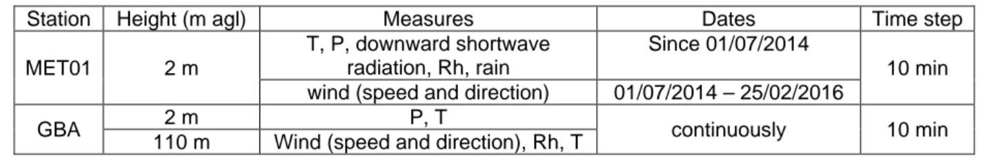
considers two wind sectors, the south-east quarter for the down-valley winds for the first class and all other directions for the second class. The PC3 considers 3 classes (Figure 2) (in blue the class of Cadarache down-valley winds (CDV), in green the class of up-valley winds and in red the class of valley transverse winds). The classes of PC being chosen based on 2 m wind directions, their values are relevant only for the low level winds in the Cadarache valley. The performances of the wind speed forecast is assessed through the correlation coefficient, bias and mean absolute error (MAE) computed between observed and predicted series.
Figure 2: Wind rose of hourly averaged observations at 2 m from Feb. 17, 2015 to Feb. 17, 2016 and classification of the winds into three direction classes (blue for down-valley winds, green for up-valley winds and red for cross-valley winds).
The comparison was done for the one year period (February 17, 2015 – February 17, 2016), which corresponds to 8760 samples (hourly forecasts).
3.2.1 Wind at 110 m
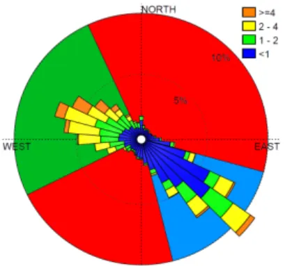
The simulated and observed wind roses (Figure 3a and 3b) display the same features, with three major wind sectors: westerly winds, north-north-easterly winds aligned with the Durance valley and south-easterly winds generally associated with cloudy/rainy weather. Concerning the directions, the DACC reaches 0.64. The probability density function (PDF) of the directions (Figure 4) confirms the overall agreement between observed and forecasted directions, with the highest PDF values concentrated in the three main sectors. However, the figure also reveals a zone of observed NE winds whereas corresponding forecasted winds cluster around CDV direction. This failed forecast provides from a bad forcing by the GFS data. Moreover, 65% of the WRF failures can be attributed to a bad forcing.
The forecasted speeds are slightly overestimated (bias of +0.98 m/s) which can be attributed to a strong overestimation in the forcing data (bias of +1.16 m/s in the GFS data).
Figure 3: Wind roses calculated with an angular resolution of 10°, for the WRF simulations (a and c) and for the observations (b and d), at the GBA (and b) and MET01 (c and d) sites. Wind speeds are in m/s.
Figure 4: Comparison of the 110 m wind direction (a) and speed (b) observed and forecasted, represented by the probability density function (color scale). The densities are calculated for wind direction groups of 10° and wind speed groups of 0.2m/s. The red, green and blue rectangles in a) correspond to the three wind sectors of Figure 2.
3.2.2 Wind at 2 m
The wind speed at 2 m is calculated from the simulated 10-m wind, assuming logarithmic profiles corresponding to neutral conditions, and compared to the observations done at the same height (MET 01 site). Wind directions at 10 m and 2 m are assumed to be equal. The valley clearly impacts the observed wind since nearly all winds are aligned with the valley axis (Figure 3d). The large-scale, westerly winds are channeled by the valley and take a north-west (up-valley) direction. The south-east winds correspond to a mix of valley-channeled winds (Duine et al., 2017)
and rainy weather conditions. This channeling is not forecasted by the model, which maintains for the wersterly and south-easterly winds the same occurrence as at 110 m. The NE Durance valley wind has disappeared, which is consistent with the observations, as already noticed by Duine et al. (2017) who showed that this flow does not appear below 100 m at the MET01 location.
The probability density function (Figure 5) shows that the west-to-north-westerly directions are correctly forecasted while down-valley winds (CDV on y-axis) are very poorly simulated since the corresponding forecasted directions spread over all the possible values.
At 2 m, the simulations produce a DACC of 0.55, a PC2 of 0.65 and a PC3 of 0.50. The wind speed is overestimated (bias of +1.09 m/s and MAE of 1.31 m/s for a mean speed of 1.39 m/s), which is probably caused by a too weak friction resulting from the smoothed topography in the simulation.
Figure 5: Same as Figure 4 but for the wind at 2 m.
3.2.3 Temperatures
Duine et al. (2016) showed that the difference of temperature between 110 m and 2 m was a good indicator of the existence of the CDV wind. Hence, it is interesting to evaluate how the forecasted temperatures compare to the GBA permanent measurements. It appears that the simulations underestimate the diurnal temperature range with a lack of heating during the day and a lack of cooling during the night, failing for example to reproduce negative temperatures at 2 m (see Fig. 6). This behavior has already been noticed by Kalverla et al. (2016) for WRF simulations of the same region. The simulation is worse for the cold temperatures than for the warm ones. The standard deviation of the difference between observations and simulations at 110 m (resp. 2 m) is 2.24°C (resp. 2.96°C) for minimum temperatures and 1.67°C (resp. 2.33°C) for maximum temperatures; however, the daily mean temperature is rather well reproduced with a bias of -0.39°C (resp. +0.17°C). From here onwards, we will analyse potential temperature difference between these two levels Δθ because this parameter is more relevant than static temperature difference to represent the stratification.
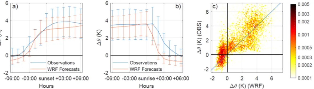
In the observations, the daily cycle of Δθ is usually well marked: the atmosphere is stably stratified during the night and unstable during the day (Figure 6). This cycle is overall well reproduced by the simulations. Before sunset, the tendencies are similar and the change of stability occurs approximately 3 h before sunset, about one hour earlier in the observations than in the simulations. The maximum observed Δθ is reached about 3 h after sunset, while in the simulations this parameter continuously strengthens all along the night. Δθ starts to decrease at sunrise in the simulations, 1 h earlier than in observations. The stable stratification period is therefore 2-hr shorter in the simulations. This difference is caused by heating (resp. cooling) at 2 m which occurs earlier (resp. later) in simulations. Though the topography is smoothed in the
model, it has been verified that this difference cannot be attributed to a shadowing effect on the observations. In the morning, the boundary layer becomes unstable 3 h earlier in simulations than in observations. Overall, Δθ is lower in simulations than in observations (negative bias of -0.56 C° and mean absolute error of 1.26 °C), and especially during the morning transition with a faster decrease of Δθ in simulations. The graph of probability density function (Figure 6c) represents the level of agreement between the observations and the simulations. It can be divided into three parts. The first one covers the observed negative Δθ (unstable stratification). In this zone, the simulated values are also negative and a large part of the values are grouped close to the 1:1 line which reflects a good agreement. The second part covers the observed values included in the range [0 - 2 C°], which corresponds to the hours preceding nightfall and following sunrise. There is a poor agreement in this range, with simulated values spread between -1 °C and 4 °C. The last part covers the observed values higher than 2 °C which corresponds to stable nighttime periods. The simulated values are positive too, but there is a large scatter showing the difficulty to accurately simulate the intensity of the stratification during the night.
Figure 6: (a): Sunset-referenced mean diurnal cycle of potential temperature difference between 110 m and 2 m. Blue color is for observations and red for simulations. Vertical bars represent standard deviations within each 1-hr time interval. (b): id. to (a) but sunrise-referenced. (c) : probability density function showing the comparison bewteen observed and forecasted potential temperature difference.
To conclude on this comparison between observations and simulations, the general behavior of vertical potential temperature difference is well reproduced for unstable as well as for very stable conditions. The winds at 110 m are pretty well reproduced, with the three main directions well forecasted. On the other hand, the forecast of the wind at 2 m is not good, especially for south-easterly winds. These winds are mostly observed during the night (density flows). Moreover, their direction is forced by the relief since they are down-valley winds (Duine et al., 2017). This is not surprising since the topography in the coarse WRF simulations is resolved for horizontal scales larger than 3 km only. Therefore, in the absence of finer-scale simulations, the forecast of local valley winds requires a statistical technique able to downscale the WRF simulations.
4. Artificial neural network 4.1 Principle and configuration used
An ANN is a statistical tool whose aim is to calculate a function linking two data sets (available on the same period). One data set (unknown variables) is considered as a target to be reproduced while the other is composed of known variables. The ANN
starts with a randomly chosen function which uses the known variables to produce a result which has to reproduce the unknown data set. This function is composed of some weighted activation functions (the so-called neurons), interconnected between each other and arranged in layers.
The two data sets are randomly divided into three sub-sets: training, validation and test. Then, the next step, applied upon the training set, consists in fitting the above-mentioned function to produce results as close as possible to the target data set. This step is iterative and lasts until the performance calculated on the validation set reaches a limit and no longer improves. Finally, the generalization degree of the ANN, that is its efficiency to produce good estimates on data sets differing from the training ones, is assessed based on the mean squared errors of the difference between true and ANN predicted values, for both the training and test sets. The two errors have to be as low and close to each other as possible (Dreyfus et al., 2002). The test set is also useful to compare different ANNs between each other.
ANNs are very good interpolators, but very poor extrapolators (Gardner and Dorling, 1998). So, the dataset used to train the ANN has to be as big and heterogeneous as possible, to include the widest range of cases that the ANN is expected to encompass.
The ANN used in this study is a Multi-Layer Perceptron (MLP) type (Beale et al., 1992). The MLP is frequently used in atmospheric sciences (Gardner and Dorling, 1998). Its specific feature is that each neuron of a layer is connected with all the neurons of the previous and next layers. It is composed of an input layer, at least one hidden layer and an output layer. Here, the input layer is composed of the training variables and there is a single hidden layer of 10 neurons (this number was chosen after scanning the ANN performance for a number of neurons varying from 5 to 50). The output layer (target) is composed of two neurons which are expected to reproduce the horizontal wind components at 2 m (u and v). The activation function is the hyperbolic tangent mathematical function, because it offered better results than other functions currently used in ANN computation, like log-sigmoid or linear functions. The dataset is randomly split, between 60% of data for the training set, 10% for the validation set and the remaining 30% for the test set, which allows us to be confident in the evaluation of the ANN performance thanks to the large amount of data composing the test set. Furthermore, the input variables are normalized between -1 and +1 before entering the ANN to avoid weight discrepancy problem that happens when the order of magnitude of variables is different.
In a first step, this ANN was applied to the KASCADE data to assess its efficiency to nowcast the wind in the Cadarache valley. The performance will be compared to the temperature threshold method of Duine et al. (2016).
4.2 Nowcasting from observations: ANN vs. threshold method
Duine et al. (2016) have developed a method to nowcast the occurrence of the CDV density current. For that purpose, they used the KASCADE observations of the wind at 10 m in the valley (from December 13, 2012 to March 16, 2013). Among the three following criteria: i) temperature difference between 110 m and 2 m, ii) wind speed at 110 m and iii) a bulk Richardson number derived from the first two variables, the first
one gave the best performance and the optimal threshold was therefore computed on this parameter. Their method produces its best result, using as criterion a temperature difference of 1.5 °C between 110 m and 2 m. Values greater than 1.5 °C are mainly associated with density down valley winds while values lower than 1.5 °C mainly correspond to winds at 10 m forced by the winds at 110 m.
In this study, this method was applied to nowcast not only the CDV density current, but every wind that can occur in the Cadarache valley. For this, the dataset used from the KASCADE observations is not exactly similar to the one Duine et al. (2016)
have used. The best result (PC2 of 0.80) was brought by the same criterion: a vertical temperature difference of 1.5°C between 110 m and 2 m.
4.3 Nowcasting CDV winds during the KASCADE period with the ANN
The ANN launched for the KASCADE period (ANNK) used four measured variables as input: Δθ, the wind speed at 110 m and the 110 m wind components, i.e. the same observations as those used by Duine et al. (2016). The global dataset is composed of 3138 samples, corresponding to a training set composed by 1883 samples, a validation set of 314 samples and a test set of 941 samples. The PC2 reaches 0.94, which is better than the Duine, et al. (2016) result of 0.91 (see Table 2
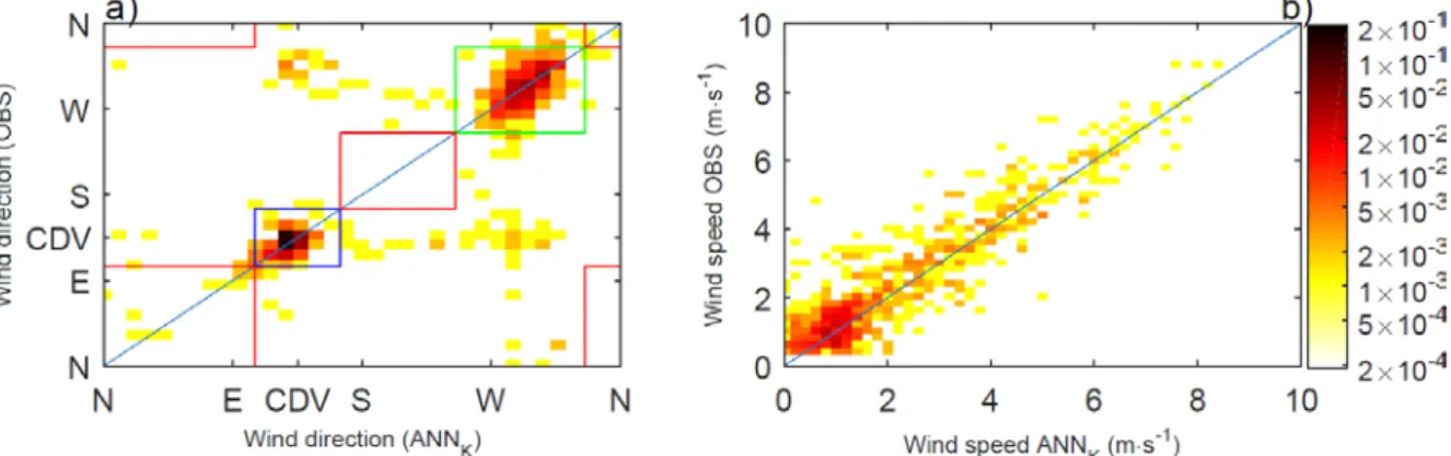
for the full results). Moreover, the ANN method provides not only the wind direction, as in Duine et al. (2016), but the two wind components from which both the speed and direction can be computed. Figure 7 presents the comparison between the observed and ANN-estimated wind speed and direction. The agreement is very good, with two hot spots (dark red areas with density > 20%) corresponding to the up valley (NW) and down valley (SE or CDV) wind directions, respectively.
Figure 7: Same as Figure 4 but for the comparison of observations to the ANNK nowcasting.
So, the ANN appears as a good tool to nowcast the low-level winds in the Cadarache valley. However, there are a few observations for which the wind directions are poorly reproduced by ANNK (see in Fig. 7a the dots outside the colored boxes). Given the very high correlation between observed and ANNK-computed wind components (0.96 and 0.93 for u and v, respectively), these defects could be attributed to very weak winds for which the directions are highly variable. The ANNK performance indexes were thus recalculated after having removed the computed wind speeds lower than 0.5 m/s. They are largely improved (row "ANNK-05" in Table 2), especially for the direction (from 0.91 to 0.96 for DACC, from 0.94 to 0.97 for PC2 and from 0.89 to 0.94 for PC3).
This allows concluding that the ANN is a suitable tool to nowcast the wind in the Cadarache valley based on above-valley observations.
4.4 Nowcasting CDV winds during a full year with the ANN
Given the encouraging results obtained on the KASCADE period, we decided to run the ANN on a full year period (from February 17, 2015 to February 17, 2016). The configuration was similar, with the same input parameters, but the observations of the CV wind were done at 2 m instead of 10 m for the KASCADE period (though at the same location). This run was called ANNOBS-yr. Like for the KASCADE period, we got excellent performances, with values of 0.94, 0.82 and 0.86, for P2, PC3 and DACC, respectively. The correlation coefficients were 0.89, 0.93 and 0.86 for the wind speed, the u and v components, respectively. The bias and MAE on the wind speed were as low as -0.17 m/s and 0.50 m/s, respectively (see Table 2). We will consider this run as a reference for the subsequent analysis of ANNs performance, as it was done on a long time series (a full year) and evaluated against in situ observations. 4.5 ANN applied to forecasting from WRF simulations
4.5.1 Searching for the most pertinent WRF variables
Among the numerous WRF output parameters, some have to be chosen as input for the ANN. Since the goal is to downscale the wind in the Cadarache valley at the MET01 position, the variables related to the larger-scale meteorological forcing and to local atmospheric stability are privileged. A first list was defined as follows:
- Pressure at 2 m above ground level - Hourly precipitation
- Relative humidity at 2 m above ground level - Short-wave and long-wave net radiation - Wind direction and speed at different heights - Wind components at 10, 20 and 100m
- Vertical potential temperature difference between 110 m and 2 m: Δθ - Boundary-layer height
- Friction velocity u*
- Bulk Richardson number between 2 m and 110 m (as in Duine et al., 2016) - Fractional time of the day
- Relative hour to closest sunset - Relative hour to closest sunrise
For the one-year period of observations, only the 2 m wind observations at MET01 are available inside the valley. So, in order to have comparable variables, the wind simulated at 10 m, has been recalculated at 2 m using a logarithmic profile derived from the wind measurements at 2 m, 10 m and 30 m collected during the KASCADE experiment at the MET01 location.
The selection of WRF-simulated variables that are used as input for the ANN is made in two steps (Dreyfus et al., 2002):
1. We computed the correlation coefficient between each possible pair of variables, and when the values were higher than 0.8the two corresponding parameters were considered as redundant and one of them was removed. The wind components at 10 m, 20 m and 100 m were highly correlated, and the two upper levels were thus removed. The friction velocity (strongly related to the boundary layer height) was also removed. Then only 14 variables remain after this first step of elimination.
2. The second step of selection consists in evaluating the impact of each variable on ANN performances. A reference ANN is launched with the 14 selected variables available as inputs (called ANNWRF14 in Table 2) and 14 other ANNs are launched, each one with removing a different variable. The less significant variables are thus identified and removed. Then, the same operation is repeated until none of the retained variable could be discarded without degrading the ANN performance. At the end of this process, 4 indispensable variables are retained: the two wind components at 10 m, the wind speed at 110 m and Δθ (discussion about their role hereafter). The final version of ANN using these variables will be called ANNWRF hereafter. 4.5.2 Performances of the ANN
The results produced by the ANNs used in this study are compiled in Table 2. The performances calculated for the WRF simulations (see above) are also included to appreciate the improvement brought in by the different ANNs.
Table 2: Summary of performances calculated for the WRF simulations and several ANNs. Mean Square Error (MSE); PC2 for 2 direction classes and PC3 for 3 classes (see Fig 2). WRF110m and WRF10m show the performances of the WRF
simulations in comparison to the observations at 110 m on the tower (GBA site on Fig. 1), and at 10 m in the valley (MET01 site on Fig. 1), respectively. ANNK and ANNK-05 show the results for the KASCADE period, the winds lower than
0.5m/s having been removed for the latter. In the rows Nr. 5 to 7, the data from the one year period have been used. ANNOBS-yr shows the performances using continuous observations as input, ANNWRF14 shows the results for the ANN
launched with 14 WRF variables and ANNWRF shows the results for the ANN using the 4 most relevant WRF variables as
input. "Gain" shows the improvement of performances brought by the ANN on the WRF output. "Loss" shows the loss of performance using WRF output rather than observations as ANN input.
Whatever the index used, the performances of the low-level wind forecast are clearly improved when the ANN is applied on WRF output (ANNWRF compared to WRF10m). The bias on the wind speed diminishes from +1.79 m/s to -0.46 m/s. The improvement on the wind direction is the best, with DACC reaching 0.75 (instead of 0.56), PC2 0.86 (instead of 0.71) and PC3 0.74 (instead of 0.53). These
improvements are also clearly visible when comparing Figure 5 and Figure 8. While the simulations alone failed to reproduce the CDV wind, resulting in a large scatter in Figure 5a, the corresponding graph for ANNWRF shows a clustering of values close to the 1:1 line (Figure 8). The failures correspond to a switching between down-valley and up-valley directions (9.2% of data set). Another striking behavior is that the neural network is only able to compute winds aligned with the main valley axis (up- or down-valley), and fails to compute cross-valley winds which are sometimes (17% of the data set) observed. Regarding the wind speed, Figure 58b highlights a small negative bias (-0.46 m/s) in the ANNWRF data, which also represents a large improvement with respect to the values produced by the WRF simulations alone (bias of +1.79 m/s, cf. Fig. 5b). The mean absolute error is similarly reduced from 2.00 m/s for the simulations alone to 0.81m/s for the ANNWRF.
Figure 8: Same as Figure 4 but for the the ANNWRF forecasts.
The improvement on the wind forecast is also visible on the probability distribution of errors on the wind direction (Q-Q plot diagram on Figure 9). The errors are lower for the ANNWRF forecast than for pure WRF simulations. As an illustration, 50% of the ANNWRF errors are in the [-20°,+20°] range, whereas 50% of the WRF errors are spread over the [-45°,+45°] range.
Figure 9: Comparison on a Q-Q diagram between the errors in degrees on wind directions for pure WRF forecasted directions
(ordinate) and for ANNWRF forecasted directions (abscissa). Each dot represents one percentile out of two and the 25th, 50th
and 75th percentile are represented by circles. 5. Discussion
5.1 Relative effect of ANN input parameters
Using only 4 variables (u10, v10, U110 and Δθ ) out of the WRF forecast as ANN input enables the ANN to calculate the 2 m wind at one spot in the Cadarache valley. However, the impact of each variable on the ANN result is different.
1. The ANN calculates the two wind components at 2 m, which explains that the WRF wind components at 10 m (the lowest level for the wind in the WRF simulations) are very important for the ANN performances. Though the WRF wind at this level is not often ill oriented because of the smoothed model topography, the correlation coefficients for the wind components reach 0.70 and 0.59 respectively for the u and v components.
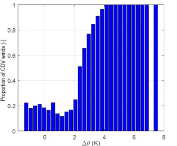
2. Duine et al. (2017) have shown the high occurrence of CDV wind over Cadarache and they have demonstrated that they are induced by stable conditions and topography. However, these winds are not well reproduced in WRF because of the smoothed topography. The use of Δθ, which is related to atmospheric stability, enables the ANN to improve the calculation of the CDV winds. Δθ is strongly connected to the down-valley wind. As long as the stratification is strengthening, the occurrence of winds going down-valley is increasing. This shows the link between the CDV wind and the stratification (Figure 10). This link was already demonstrated by Duine et al. (2017) for the Cadarache valley.
3. Removal of the wind speed at 110 m degrades several performance indexes, which makes this variable useful for the calculation. At 110 m, the wind speed can be considered as a good indicator of forcing above the Cadarache valley which is impacting for stability and wind in the valley.
__
Figure 10: Proportion of ANNWRF-computed CDV winds as a function of the WRF-computed vertical potential temperature
difference.
5.2 ANN strengths and weaknesses
Figure 8 already highlighted some limitations on the forecasting of winds not aligned with the valley axis. This is also illustrated in Figure 11, which shows the occurrences of the two wind components, in the observations and forecasted by the ANNWRF model. Besides the narrowness of the two main directions on the simulated winds, with respect to the observed ones, the plots also reveal a non-alignment of the two opposite winds: the down-valley winds are parallel to the main axis of the valley, whereas the "up-valley" directions cluster around ~280°, i.e. a ~25° backing from the valley axis. This behavior, mainly observed during the day, is related to larger-scale
çforcing (Mistral conditions, see e.g. the wind rose on Fig. 2), when turbulence transports momentum from upper levels close to the surface, thus lowering the channeling effect of the local valley.
Furthermore, the ANN performance is improved when the wind speed strengthens (see Figure 12 and the comparison between ANNK and ANNK-05 in Tab. 2). Up to 3.6 m/s, there is always a 100% performance considering the DACC value. There are two reasons for this. Firstly, this is due to the method used to calculate the wind direction, which is not directly calculated by the ANN (as it is not possible to compute cyclic functions through ANN), but derived from wind components. All things being equal, a small error made on one component for lower winds produces a higher error on the wind direction than for stronger winds. Moreover, it is well know that the directions are not well defined for the low winds (Jarraud, 2008). Then, the difficulty to calculate the directions for low winds is another explanation for the bad representation of winds orthogonal to the valley (mean wind speed of 0.66 m/s for these winds against 1.10 m/s for the CDV winds and 2.08 m/s for the up-valley winds), which in turn justifies the discarding of low speed winds (< 0.5m/s) calculated by the ANN.
Figure 11: Probability density of wind components observed (a) and calculated by ANNWRF (b). The blue lines and the
corresponding labels indicate the wind directions. The cyan line shows the direction of the valley axis. The dotted circles represent the wind speeds, spaced by 1 m/s, and the black one represents 0.5 m/s.
Figure 12: DACC values as a function of the wind speed calculated by the ANNWRF (blue bars and left ordinate scale), and
number of data in each wind speed bin (black line and right ordinate scale).
Another parameter investigated as possibly impacting the performances of an ANN is the quality of input data.
The high performance reached by the ANNOBS-yr shows the efficiency of an ANN to calculate a local wind, with a low error, using observations. But, using forecasted data (containing their own forecasting errors) as input increases the ANN error which explains the higher performances of the ANNOBS-yr compared to the ANNWRF. Thereby, the ANN error due to the forecasting error was estimated ("Loss" line in
Table 2). Although the loss of performance of the ANNWRF is not negligible, the gain brought compared to the pure WRF simulations remains very appreciable.
6. Conclusion
The aim of this study was to complement WRF mesoscale simulations in order to predict a local wind mostly forced by subgrid-scale orographic effects unaccessible in WRF given the horizontal resolution of the model (3 km). In particular, during stable stratification periods when the larger-scale forcing is low, a density current whose direction is constrained by a small valley (1 km width) is regularly observed but not forecasted. Since the overall stratification is pretty well reproduced in the mesoscale simulations, a statistical downscaling has been elaborated using an artificial neural network, the performance of which was evaluated against observations done at one spot inside the valley.
Artificial neural networks are powerful statistical tools allowing to represent complex non-linear phenomena. For that purpose, they are generally trained and evaluated with observations. In this study, the observations done during the 3-month KASCADE experiment, at a height larger than the valley depth and therefore representative of the non-local flow, have been used in a first step to evaluate the ANN capability to infer the wind inside this small valley. The ANN got excellent results, surpassing a statistical nowcasting method developed formerly upon the same dataset by Duine et al. (2016).
The next step was to apply the ANN technique to the output of the WRF model run in an operational mode with a 3-km horizontal resolution. For every day during a full year, the 24-to-48 hr forecast period was used as input to the ANN. The observations, available during this 1-yr period, consisted in wind speed and direction measured at 2 m agl in the central part of the small Cadarache valley. These observations served to train the ANN. One year of data constitute a large enough dataset to encompass most of the meteorological conditions representative of Cadarache.
Thanks to the 1-yr observations, and to the continuous observation done on the Cadarache site (wind and temperature at 110 m on a tower, and temperature at 2 m), the overall performance of the WRF simulations was first evaluated. Not surprisingly, the wind at 2 m is not well forecasted due to the lack of local topography in the simulations. On the other hand, the wind at 110 m and the temperature difference between 2 m and 100 m are pretty well forecasted, showing that some parameters, poorly related to the local topography, can be well reproduced even with a coarse horizontal resolution. This encouraged us to feed an ANN with such parameters in order to forecast the local valley winds. With respect to the downscaling, nowcasting technique developed by Duine et al. (2016), we went a step further with the possibility to forecast the local valley winds.
Hence, several WRF variables were tested to feed the ANN. After elimination of redundant parameters, as well as of the parameters whose impact on the result was weak, four of them were definitely retained (the wind components at 10 m, the difference in potential temperature between 110 m and 2 m, and the wind speed at 110 m).
The ANN significantly improved the forecast of the wind in the Cadarache valley, for both the speed and direction. The scores obtained for the full year were 0.75 for DACC, 0.86 and 0.74 for PC2 and PC3, respectively, the bias on wind speed was 0.46 m/s and the MAE 0.81 m/s. We have coped with the main failure observed in the WRF simulations, concerning the valley winds: the wind direction is now satisfactorily forecasted and the important bias on the speed is considerably decreased.
The ANN performance is improved as long as the wind speed increases. This is probably related to the fact that the ANN output is not the direction itself (against which the performance is evaluated), but the two wind components, from which the direction is computed. Furthermore, the strong directional pattern of the wind observed (with 78% of winds aligned along two main directions) brings the ANN to miss the winds differing from these two directions.
In conclusion, the artificial neural network technique is a valuable tool to downscale the output files of the numerical simulations and forecast the local flows at a scale which is not resolved by the model. A set of observations, large enough to encompass the variability of the meteorological conditions observed at a given location, is required to the training step of the ANN used. The ANN technique can thus be used to estimate the local flows either from continuous observations representative of a larger scale, as in Duine et al. (2016), or from operational weather forecast model whose resolution is too coarse to take into account the local influence of the topography, land use, etc.. To our knowledge, this promising technique has not
been previously used on routinely forecasted meteorological fields, though its high potential for weather as well as air quality concerns.
Acknowledgements
Bastin, S., Drobinski, P., Dabas, A., Delville, P., Reitebuch, O., & Werner, C. (2005). Impact of the Rhône and Durance valleys on sea-breeze circulation in the Marseille area. Atmospheric
research, 74(1), 303-328.
Beale, M. H., Hagan, M. T., & Demuth, H. B. (1992). Neural Network Toolbox™ Getting Started Guide.
Berthou S [et al.] Influence of submonthly air–sea coupling on heavy precipitation events in the Western Mediterranean basin [Journal]. - 2016.
Burns P and Chemel C Interactions between downslope flows and a developing cold-air pool [Journal]. - 2014.
Cadenas, E., & Rivera, W. (2009). Short term wind speed forecasting in La Venta, Oaxaca, México, using artificial neural networks. Renewable Energy, 34(1), 274-278.
Chow F, De Wekker S and Snyder B Mountain weather research and forecasting [Book]. - 2013. Clements C, Whiteman C and Horel J Cold-air-pool structure and evolution in a mountain basin: Peter sinks, Utah [Journal]. - 2003.
Clements, W. E., Archuleta, J. A., & Gudiksen, P. H. (1989). Experimental design of the 1984 ASCOT field study. Journal of Applied Meteorology, 28(6), 405-413.
Coulibaly, P., Y. B. Dibike and F. Anctil, 2005: Downscaling precipitation and temperature with temporal neural networks. J. Hydrometeor., 6, 483–495.
Cros, B., Durand, P., Cachier, H., Drobinski, P., Frejafon, E., Kottmeier, C., ... & Saıd, F. (2004). The ESCOMPTE program: an overview. Atmospheric Research, 69(3), 241-279.
Delon, C., Serça, D., Boissard, C., Dupont, R., Dutot, A., Laville, P., ... & Delmas, R. (2007). Soil NO emissions modelling using artificial neural network. Tellus B, 59(3), 502-513.
Doran, J. C., Fast, J. D., & Horel, J. (2002). The VTMX 2000 campaign. Bulletin of the American Meteorological Society, 83(4), 537-551.
Dreyfus, G., Martinez, J. M., Samuelides, M., Gordon, M. B., Badran, F., Thiria, S., & Hérault, L. (2002). Réseaux de neurones-Méthodologie et applications.
Duine Gert-Jan Characterization of down-valley winds in stable stratification from KASCADE field campaign and WRF mesoscale simulations [Rapport]. - 2015.
Duine G-J [et al.] A simple method based on routine observations to nowcast down-valley flows in shallow, narrow valleys [Revue]. - 2016a.
Duine G-J [et al.] A simple method based on routine observations to nowcast down-valley flows in shallow, narrow valleys [Revue]. - 2016a.
Duine G-J [et al.] Down-valley flows in stable stratification - Observations in complex terrain during the KASCADE fiel experiment [Journal]. - 2016b.
Fernando, H. J. S., Pardyjak, E. R., Di Sabatino, S., Chow, F. K., De Wekker, S. F. J., Hoch, S. W., ... & Steenburgh, W. J. (2015). The MATERHORN: Unraveling the intricacies of mountain
weather. Bulletin of the American Meteorological Society, 96(11), 1945-1967.
Gardner, M. W., & Dorling, S. R. (1998). Artificial neural networks (the multilayer perceptron)—a review of applications in the atmospheric sciences. Atmospheric environment, 32(14), 2627-2636. Jarraud, M. (2008). Guide to meteorological instruments and methods of observation (WMO-No. 8). World Meteorological Organisation: Geneva, Switzerland.
Kalverla, P. C., Duine, G. J., Steeneveld, G. J., & Hedde, T. (2016). Evaluation of the Weather Research and Forecasting model in the Durance Valley complex terrain during the KASCADE field campaign. Journal of Applied Meteorology and Climatology, 55(4), 861-882.
Lareau N P [et al.] The persistent cold-air pool study [Journal]. - 2013.
Largeron Y Dynamique de la couche limite atmosphérique stable en relief complexe. Application aux épisodes de pollution particulaire des vallées alpines. [Revue]. - 2010.
Liu, X. and P. Coulibaly, “Downscaling ensemble weather predictions for improved week-2 hydrologic forecasting,” Journal of Hydrometeorology, vol. 12, no. 6, pp. 1564–1580, 2011.
More, A., & Deo, M. C. (2003). Forecasting wind with neural networks. Marine structures, 16(1), 35-49.
Muñoz Ricardo C [et al.] Strong down-valley low-level jets over the atacama desert: observational characterization [Book]. - 2013.
Paci, A., & Staquet, C. (2016, April). The Passy-2015 field experiment: wintertime atmospheric dynamics and air quality in a narrow alpine valley. In EGU General Assembly Conference Abstracts (Vol. 18, p. 3162).
Philippopoulos, K., & Deligiorgi, D. (2012). Application of artificial neural networks for the spatial estimation of wind speed in a coastal region with complex topography. Renewable Energy, 38(1), 75-82.
Pope S Turbulent flows [Book]. - 2001.
Price J [et al.] Colpex: field and numerical studies over a region of small hills [Revue]. - 2011. Santos-Alamillos F. J., Pozo-Vázquez, D., Ruiz-Arias, J. A., Lara-Fanego, V., & Tovar-Pescador, J Analysis of WRF model wind estimate sensitivity to physics parameterization choice and terrain representation in Andalusia (Southern Spain) [Revue]. - 2013.
Simpson John E Sea breeze and local winds [Ouvrage]. - 1994.
Skamarock W and Klemp J A time nonhydrostatic model for weather research and forecasting applications [Journal]. - 2008.
Whiteman C and Doran J The relationship between overlying synoptic-scale flows and winds within a valley [Journal]. - 1993.
Whiteman, C. D., Hoch, S. W., Hahnenberger, M., Muschinski, A., Hohreiter, V., Behn, M., ... & Clements, C. B. (2008). METCRAX 2006: Meteorological experiments in arizona's meteor crater. Bulletin of the American Meteorological Society, 89(11), 1665-1680.
Wyngaard J Toward numerical modeling in the "Terra incognita" [Journal]. - 2004.
Hu, Q., Zhang, R., & Zhou, Y. (2016). Transfer learning for short-term wind speed prediction with deep neural networks. Renewable Energy, 85, 83-95.
Liu, H., Tian, H., Liang, X., & Li, Y. (2015). New wind speed forecasting approaches using fast
ensemble empirical model decomposition, genetic algorithm, Mind Evolutionary Algorithm and Artificial Neural Networks. Renewable Energy, 83, 1066-1075.