A consistent model for πN transition distribution amplitudes
and backward pion electroproduction
J. P. Lansberg1, B. Pire2, K. Semenov-Tian-Shansky2,3,4, L. Szymanowski5 1 IPNO, Universit´e Paris-Sud, CNRS/IN2P3, 91406 Orsay, France
2 CPhT, ´Ecole Polytechnique, CNRS, 91128 Palaiseau, France 3 LPT, Universit´e Paris-Sud, CNRS, 91404 Orsay, France 4 IFPA, d´epartement AGO, Universit´e de Li`ege, 4000 Li`ege, Belgium
5 National Center for Nuclear Research (NCBJ), Warsaw, Poland
Abstract
The extension of the concept of generalized parton distributions leads to the introduction of baryon to meson transition distribution amplitudes (TDAs), non-diagonal matrix elements of the nonlocal three quark operator between a nucleon and a meson state. We present a general framework for modelling nucleon to pion (πN ) TDAs. Our main tool is the spectral representation for πN TDAs in terms of quadruple distributions. We propose a factorized Ansatz for quadruple distributions with input from the soft-pion theorem for πN TDAs. The spectral representation is complemented with a D-term like contribution from the nucleon exchange in the cross channel. We then study backward pion electroproduction in the QCD collinear factorization approach in which the non-perturbative part of the amplitude involves πN TDAs. Within our two component model for πN TDAs we update previous leading-twist estimates of the unpolarized cross section. Finally, we compute the transverse target single spin asymmetry as a function of skewness. We find it to be sizable in the valence region and sensitive to the phenomenological input of our πN TDA model.
1. INTRODUCTION
The familiar collinear factorization theorem [1, 2] for exclusive electroproduction of pions off nucleons
e(k) + N(p1) →
¡
γ∗(q) + N(p1)
¢
+ e(k0) → e(k0) + π(pπ) + N0(p2), (1)
valid in the generalized Bjorken limit (large Q2 = −q2 and s ≡ (p
1+ q)2; xB = Q 2 2p1·q and skewness variable ξ = −(p2−p1)·n (p1+p2)·n being fixed 1; and small −t ≡ (p
2− p1)2) gives rise to the
description of this reaction in terms of the generalized parton distributions (GPDs) (see left panel of Fig. 1) .
According to a conjecture made in [3, 4], a similar collinear factorization theorem for the reaction (1) should be valid in the following complementary kinematical regime:
• large Q2 and s;
• fixed xBand skewness variable ξ, which is now defined with respect to the u-channel
momentum transfer:
ξ = −(pπ− p1) · n
(pπ+ p1) · n
; (2)
• the u-channel momentum transfer squared u ≡ (pπ − p1)2 (rather than t) is small
compared to Q2 and s.
Under these assumptions, the amplitude of the reaction (1) factorizes as it is shown on the right panel of Fig.1. This requires the introduction of supplementary non-perturbative objects in addition to GPDs – nucleon to pion transition distribution amplitudes (πN TDAs). Technically, πN TDAs are defined through the πN matrix element of the tri-local three quark operator on the light cone [5–9]:
b Oαβγ ρτ χ(λ1n, λ2n, λ3n) = εc1c2c3Ψ c1α ρ (λ1n)[λ1n; λ0n]Ψcτ2β(λ2n)[λ2n; λ0n]Ψcχ3γ(λ3n)[λ3n; λ0n] . (3)
1 n is the conventional light-cone vector occurring in the Sudakov decomposition of the relevant
Here α, β, γ stand for quark flavor indices and ρ, τ , χ denote the Dirac spinor indices. Antisymmetrization stands over the color group indices c1,2,3. Gauge links may be omitted
in the light-like gauge A · n = 0.
p1 p2 pπ CF GP D DA γ∗ t s Q2 p1 pπ p2 CF0 πN T DA DA0 γ∗ u s Q2
FIG. 1: Left: Collinear factorization for hard production of pions in the conventional hard meson production kinematics. Right: Collinear factorization for hard production
of pions off nucleons in the backward kinematics.
The detailed account of this approach is presented in Refs. [10–12]. Apart from the description of hard exclusive pion electroproduction off a nucleon in the backward region, the same non-perturbative objects appear in the collinear factorized description of differ-ent exclusive reactions. Promindiffer-ent examples are baryon-antibaryon annihilation into a pion and a lepton pair in the forward and backward directions [13–15].
The physical picture encoded in baryon to meson TDAs is conceptually close to that contained in baryon GPDs and baryon distribution amplitudes (DAs). Baryon to meson TDAs are matrix elements of a three quark operator (i.e. with baryonic number one) and characterize partonic correlations inside a baryon. This gives access to the momentum distribution of the baryonic number inside a nucleon. The same operator also defines the nucleon DA which can be seen as a limiting case of baryon to meson TDAs with the meson state replaced by the vacuum. In the language of the Fock state decomposition, baryon to meson TDAs are not restricted to the lowest Fock state as DAs. They rather probe the non-minimal Fock components with additional quark-antiquark pair:
|Nucleoni = |ΨΨΨi + |ΨΨΨ; ¯ΨΨi + .... ;
For baryon to meson TDAs one may distinguish the Efremov-Radyushkin-Brodsky-Lepage (ERBL)-like domain in which all three momentum fractions of quarks are posi-tive and two kinds of Dokshitzer-Gribov-Lipatov-Altarelli-Parisi (DGLAP)-like regions in which either one or two momentum fractions of quarks are negative. On Fig. 2, we show the interpretation of πN TDAs in the ERBL-like and in DGLAP-I,II region within the light-cone quark model [16]. As one can see from Fig.2 (a) the ERBL part is probing the non-minimal Fock components of the nucleon wave function. In the DGLAP-II Fig. 2 (c) region one rather probes the non-minimal Fock components of the meson state, while in the DGLAP-I Fig. 2 (b) region there is a non-vanishing contribution of the minimal Fock states of baryon and meson. This interpretation, obviously, is justified only at a very low normalization scale. The evolution effects may significantly change it at higher scales.
Ψ Ψ Ψ ¯ Ψ Ψ Ψ ¯ Ψ x1 x2 x3 (a) Ψ Ψ Ψ Ψ ¯ Ψ x1 x2 x3 (b) Ψ Ψ Ψ Ψ ¯ Ψ x1 x2 x3 Ψ ¯ Ψ (c)
FIG. 2: Interpretation of πN TDAs within the light-cone quark model [16]. Small vertical arrows show the flow of the momentum. (a): Contribution in the ERBL region
(all xi are positive); (b): Contribution in the DGLAP I region (one of xi is negative).
(c): Contribution in the DGLAP II region (two xi are negative).
Similarly to GPDs [17–19], by Fourier transforming πN TDAs to the impact parameter space (∆T → bT), one obtains additional insight on the nucleon structure in the transverse
plane. This allows one to perform the femto-photography of hadrons [20] from a new perspective. In particular, there are hints [21] that πN TDAs may be used as a tool to perform spatial imaging of the structure of the meson cloud of the nucleon. This point, which still awaits a detailed exploration, opens a fascinating window for the investigation of the various facets of the nucleon interior.
Our paper is organized as follows: In Sec. 2, we provide a short summary of the basic properties of πN TDAs. In Sec. 3, we review the spectral representation for πN TDAs and propose a factorized Ansatz for the quadruple distributions constrained by the soft pion theorem for πN TDAs. We complement the spectral representation with a D-term like contribution and build a two component model for πN TDAs. Sec. 4 contains the details of calculation of γ∗N → πN amplitude in the backward regime. In Sec. 5, we
compute the unpolarized cross section and transverse target single spin asymmetry of backward π+ and π0 electroproduction off protons using our two component model for
πN TDAs. Many technical details are relegated to Appendices A-D. Our conclusions are
presented in Sec. 6.
2. GENERAL PROPERTIES OF πN TDAS
At the leading twist-3, the parametrization of the Fourier transform of πN matrix elements of the three-local light-cone quark operator (3) can be written as
4(P · n)3 Z "Y3 j=1 dλj 2π # eiP3k=1xkλk(P ·n)hπ a(pπ)| bOρ τ χαβγ(λ1n, λ2n, λ3n)|Nι(p1)i = δ(x1 + x2+ x3− 2ξ) X s.f. (fa)αβγι sρ τ, χHs.f.(πN )(x1, x2, x3, ξ, ∆2; µ2F) , (5) where P = p1+pπ
2 is the average momentum and ∆ = pπ− p1 is the u-channel momentum
transfer. The spin-flavor (s.f.) sum in (5) stands over all independent flavor structures (fa)αβγι and the Dirac structures sρ τ, χ relevant at the leading twist; ι (a) is the nuclon
(pion) isotopic index. The invariant amplitudes Hs.f.(πN ), which are often referred to as the leading twist πN TDAs, are functions of the light-cone momentum fractions xi (i =
1, 2, 3), the skewness variable ξ (2), the u-channel momentum-transfer squared ∆2 and
For given isotopic contents (say proton to π0 TDA), the parametrization (5) of twist-3
πN TDAs involves 8 invariant functions V1,2(πN ), A(πN )1,2 , T1,2,3,4(πN ) (see Eq. (A1)). However, not all of them are independent. Taking into account the isotopic and permutation symmetries (see [12]), one may check that in order to describe all isotopic channels of the reaction (1), it suffices to introduce eight independent πN TDAs: four in the isospin-1
2 channel
and four in the isospin-3
2 channel. This result is analogous to the case of leading twist
nucleon DAs: initially, the parametrization [9] involves three proton DAs Vp, Ap and Tp.
However, due to the isotopic and permutation symmetries, these three functions may be expressed through the unique leading twist nucleon DA φN ≡ Vp− Ap. Neutron DAs are
expressed as {Vn, An, Tn} = {−Vp, −Ap, −Tp}.
The support domain of baryon to meson TDAs in the light-cone momentum fractions xi
(Pixi = 2ξ) was established in [11]. It is given by the intersection of three stripes −1+ξ ≤
xi ≤ 1 + ξ. Instead of dealing with three dependent light-cone momentum fractions xi,
one can switch to the independent variables. A convenient choice of independent variables is the use of the so-called quark-diquark coordinates [11]. Due to the symmetry of the support of baryon to meson TDAs under rotations by the 2π
3 angle, there exist three
equivalent choices of quark-diquark coordinates (i = {1, 2, 3}):
wi = xi− ξ; vi = 1 2 3 X k,l=1 εiklxk, (6)
where εikl is the totally antisymmetric tensor. The support domain of baryon to meson
TDAs in terms of quark-diquark coordinates can be parameterized as:
− 1 ≤ wi ≤ 1 ; −1 + |ξ − ξi0| ≤ vi ≤ 1 − |ξ − ξi0| , (7)
where ξ0
i ≡ ξ−wi2 .
As pointed out in [14], the scale dependence of πN TDAs is described by the appropri-ate generalization of the ERBL/DGLAP evolution equations. Splitting functions in this case turn out to be much more complicated, as they include different pieces in different (ERBL-like and DGLAP-like) kinematical regions.
Exactly as for the case of the usual parton distributions and GPDs, evolution of πN TDAs can also be treated in terms of renormalization of local operators corresponding to the Mellin moments of πN TDAs in x. Evolution properties of the local operators
in question were extensively studied in connection with the scale dependence of nucleon DAs (see Refs. [22, 23]). The conformal partial wave expansion of πN TDAs over the conformal basis of the Appel polynomials or the Jacobi and Gegenbauer polynomials represents an alternative strategy for the parametrization of πN TDAs in the spirit of the dual representation of GPDs [24, 25] or complex conformal partial wave expansion [26].
Similarly to the GPD case, the polynomiality property in ξ of the Mellin moments of πN TDAs in the light-cone momentum fractions xi is the direct consequence of the
underlying Lorentz symmetry. For n1 + n2 + n3 = N the highest power of ξ occurring
in the (n1, n2, n3)-th Mellin moment of V1,2πN, AπN1,2, T1,2πN is N + 1, while for T3,4πN it is N.
Consequently, TDAs VπN
1,2 , AπN1,2, T1,2πN include an analogue of the D-term contribution [27],
which generates the highest possible power of ξ.
The most direct way to ensure both the polynomiality and the support properties for
πN TDAs is to employ the spectral representation in terms of quadruple distributions,
generalizing the familiar Radyushkin’s double distribution representation for GPDs [28– 31]. In phenomenological applications, an inviting strategy, which proved to be successful in the case of GPDs, is to construct a factorized Ansatz for the corresponding spectral densities. However, contrary to the GPD case, πN TDAs lack a comprehensible forward limit, ξ → 0. This hampers the construction of the hypothetic factorized Ansatz for quadruple distributions with input at ξ = 0 as suggested in [11].
In this paper, we build up a consistent model for πN TDAs relying on their chiral properties. Chiral dynamics constrains πN TDAs in the opposite limit, ξ → 1. Indeed,
πN TDAs are conceptually much related to pion-nucleon generalized distribution
ampli-tudes (πN GDAs), which are defined through the cross-conjugated matrix element of the same three quark operator (3):
h0| bOαβγ
ρ τ χ(λ1n, λ2n, λ3n)|Nι(p1)πa(−pπ)i . (8)
A similar correspondence was previously established between pion GPDs and 2π GDAs [27, 32]. For simplicity, let us consider the pion to be massless (m = 0). In this case the point ξ = 1, ∆2 = M2, where M stands for the nucleon mass, belongs simultaneously to
both physical regions: that of πN GDAs and that of πN TDAs (see discussion in [12]). Moreover, it is at this very point that the soft-pion theorem [33] applies for πN GDAs. As argued in [34, 35], this allows us to express πN GDAs at the threshold in terms of
the nucleon DAs Vp, Ap and Tp. In the chiral limit, the soft-pion theorem for GDAs also
constrains πN TDAs similarly to the way [36] the soft-pion theorem [32] for 2π GDAs in the chiral limit links the isovector pion GPD at ξ = 1, ∆2 = 0 to the pion DA ϕ
π.
In the chiral limit, the soft-pion theorem thus provides the normalization point for πN TDAs. The explicit form of the soft-pion theorem for πN TDAs was established in [12]. In this paper, we use this information as input for realistic modelling of πN TDAs based on the spectral representation in terms of quadruple distributions.
3. SPECTRAL REPRESENTATION FOR πN TDAS, FACTORIZED ANSATZ
FOR QUADRUPLE DISTRIBUTIONS AND D-TERM
In this section, we propose a two component model for πN TDAs involving the following contributions:
1. a spectral representation with input fixed at ξ = 1 from the soft-pion theorem; 2. a nucleon-pole exchange in the u-channel which is a pure D-term like contribution
complementary to the spectral representation.
To do so, we formulate the spectral representation constructed in [11] in a way suitable for the implementation of chiral constraints for πN TDAs. This allows us to propose a factorized Ansatz for quadruple distributions with input from the soft-pion theorem.
1. Toy exercise: GPD case
To give an idea of the new type of factorized Ansatz for quadruple distributions, let us first consider how one can constrain a GPD model from the ξ = 1 limit rather than from the forward limit ξ = 0. Let us consider the standard double distribution (DD) representation for GPDs [28–31]:
H(x, ξ) =
Z
Ω
dβdα δ(x − β − αξ)f (β, α), (9)
where Ω is the usual domain in the spectral parameter space
and f (β, α) is the double distribution. Let us perform the change of variables: α = κ+θ 2 , β = κ−θ 2 . This gives: H(x, ξ) = Z 1 −1 dκ Z 1 −1 dθ δ µ x +1 − ξ 2 θ − 1 + ξ 2 κ ¶ 1 2F (κ, θ) , (11) where F (κ, θ) ≡ f ³ κ−θ 2 , κ+θ2 ´
. Instead of the usual factorized Ansatz in (9) in the variables {β, α},
f (β, α) = h(β, α)q(β), (12)
let us employ in (11) the following factorized Ansatz in the variables {κ, θ}:
F (κ, θ) = 2ϕ(κ)h(θ), (13)
with the profile h(θ) normalized according to Z 1
−1
dθh(θ) = 1 . (14)
Obviously, Eq. (11) then gives H(x, ξ = 1) = ϕ(x).
In order to implement the so-called “Munich symmetry” [37] f (β, α) = f (β, −α), which is the consequence of hermiticity and time-reversal invariance of non-forward matrix element entering the definition of GPDs, one should require that
h(θ) ≡ ϕ(−θ) ·Z 1 −1 dθϕ(−θ) ¸−1 . (15)
Let us emphasize that, in the GPD case, symmetry requirements unambiguously fix the shape of the profile h in the factorized Ansatz (13).
Although it is but a toy model, the factorized Ansatz (13) may be applied to the case of quark isovector GPD of a pion Hu−d
π , which in the soft-pion limit [32] reduces to the
pion DA ϕπ:
lim
ξ→1H u−d
2. An alternative form of the spectral representation for πN TDAs
Let us now apply the trick of previous subsection for the case of πN TDAs. According to [11], the spectral representation for πN TDAs reads:
H(πN )(x1, x2, x3 = 2ξ − x1− x2, ξ) = " 3 Y i=1 Z Ωi dβidαi # δ(x1− ξ − β1 − α1ξ) δ(x2− ξ − β2− α2ξ) ×δ(β1 + β2+ β3)δ(α1+ α2+ α3+ 1)f (β1, β2, β3, α1, α2, α3), (17)
where Ωi denote three copies of the usual domain (10) in the spectral parameter space.
The spectral density f is an arbitrary function of six variables, which are subject to two constraints imposed by the two last delta functions in eq. (17). Therefore, f is effectively a quadruple distribution. The spectral representation (17) by the very construction ensures the polynomiality and the support properties of πN TDAs.
Let us employ the particular choice of the quark-diquark coordinates (wi, vi) (6) and
introduce the following combinations of the spectral parameters:
κi = αi+ βi; θi = 1 2 3 X k,l=1 εikl(αk+ βk); µi = αi− βi; λi = 1 2 3 X k,l=1 εikl(αk− βk). (18)
The spectral representation (17) can then be rewritten as:
H(wi, vi, ξ) = Z 1 −1 dκi Z 1−κi 2 −1−κi2 dθi Z 1 −1 dµi Z 1−µi 2 −1−µi2 dλiδ(wi− κi− µi 2 (1 − ξ) − κiξ) ×δ µ vi− θi− λi 2 (1 − ξ) − θiξ ¶ 1 4Fi(κi, θi, µi, λi). (19) The working formulas for the calculation of πN TDAs in the ERBL-like and DGLAP-like domains are summarized in Appendix B 2.
We suggest using the following factorized Ansatz for the quadruple distribution Fi in
(19):
with the profile function h(µi, λi) normalized as Z 1 −1 dµi Z 1−µi 2 −1−µi2 dλih(µi, λi) = 1. (21)
Note that the support of the profile function h is that of a baryon DA.
With the help of the spectral representation (19), one can check that in the limit ξ → 1
Hi now reduces to
H(wi, vi, ξ = 1) = V (wi, vi). (22)
We also note that the support properties of Fi(κi, θi, µi, λi) in the (κi, θi)-plane
corre-spond to that of baryon DAs. It is thus natural to use the combination of baryon DAs to which πN TDA reduces in the limit ξ → 1 due to the soft-pion theorem as input for
V (wi, vi).
Let us denote the combination of nucleon DAs, to which πN TDA H reduces in the limit
ξ → 1, as V (y1, y2, y3). It is the function of three momentum fractions yi (0 ≤ yi ≤ 1)
satisfying the condition Piyi = 1. Then, according to the particular choice of
quark-diquark coordinates in (17), one has to employ in (20):
V (κ1, θ1) ≡ 1 4V µ κ1+ 1 2 , 1 − κ1+ 2θ1 4 , 1 − κ1− 2θ1 4 ¶ ; V (κ2, θ2) ≡ 1 4V µ 1 − κ2− 2θ2 4 , κ2+ 1 2 , 1 − κ2 + 2θ2 4 ¶ ; V (κ3, θ3) ≡ 1 4V µ 1 − κ3+ 2θ3 4 , 1 − κ3− 2θ3 4 , κ3+ 1 2 ¶ . (23)
The profile function h(µi, λi) also has the support of a baryon DA: −1 ≤ µi ≤ 1;
−1−µi2 ≤ λi ≤ 1−µi2 . Contrary to the GPD case, no symmetry constraint from hermiticity
and time-reversal invariance occurs for quadruple distributions. Therefore, we are free to employ an arbitrary shape for the profile function. For example, we may assume that it is determined by the asymptotic form of a baryon DA (120y1y2y3 with
P iyi = 1): h(µi, λi) = 15 16(1 + µi)((1 − µi) 2− 4λ2 i) . (24)
In fact, this is the simplest possible choice for the profile vanishing at the borders of its domain of definition. The normalization (21) is obviously ensured.
On Fig. 3, we present the result of the calculation of π0p TDAs from the factorized
w ≡ w3, v ≡ v3 defined in (6). In accordance with the soft-pion theorem, in the ξ = 1
limit, our π0p TDAs Vπ0p
1 , Aπ
0p
1 and Tπ
0p
1 are reduced to the following combination of
nucleon DAs [12]2: V1π0p(x1, x2, x3, ξ = 1) = − 1 2 × 1 4V p³x1 2 , x2 2, x3 2 ´ ; Aπ10p(x1, x2, x3, ξ = 1) = − 1 2 × 1 4A p³x1 2 , x2 2, x3 2 ´ ; T1π0p(x1, x2, x3, ξ = 1) = 3 2 × 1 4T p³x1 2 , x2 2 , x3 2 ´ . (25)
We employ the Chernyak-Zhitnitsky (CZ) nucleon DA [41] as the numerical input. Our spectral representation provides a lively xi and ξ dependence for πN TDAs.
How-ever, the suggestion of a reasonable ∆2 dependence still remains an open question. The
most straightforward solution would be, similarly to early attempts in the GPD case, to try a sort of factorized form of ∆2 dependence for quadruple distributions (20):
Fi(κi, θi, µi, λi, ∆2) = 4V (κi, θi) h(µi, λi) × G(∆2), (26)
where G(∆2) is the πN transition form factor of the local three quark operator
b
Oαβγ
ρτ χ(0, 0, 0) (3). This leads to a factorized ∆2-dependence for πN TDAs:
HπN(x
i, ξ, ∆2) = HπN(xi, ξ) × G(∆2). (27)
The determination of G(∆2) goes beyond the scope of the present paper. Let us however
note that such a factorized form of the ∆2 dependence is known to be oversimplified and
was much criticized in the GPD case (see e.g. discussion in [38]).
2 Note that eq. (11) of [15] and eq. (19) of [10] contain a sign error for Tπ0p
as well as erroneous overall factors 2. This affects the numerical results of these papers.
FIG. 3: π0p TDAs Vπ0p
1 , Aπ
0p
1 and Tπ
0p
1 computed in the model based on the factorized
Ansatz (20) with the profile function (24) as functions of quark-diquark coordinates w ≡
w3, v ≡ v3. In the limit ξ = 1, as required by the soft-pion theorem, TDAs are reduced to
the appropriate combinations of nucleon DAs Vp, Ap and Tp (see eq. 25). For ξ < 1, πN
TDAs are obtained by “skewing” ξ = 1 limit. CZ nucleon DAs [41] are used as numerical input.
3. D-term-like nucleon pole contribution
Similarly to the GPD case, πN TDAs within the spectral representation (17) do not satisfy the polynomiality condition in its complete form. As it was pointed out in [12], the spectral representation for πN TDAs V1,2(πN ), A(πN )1,2 , T1,2(πN ) has to be complemented by an analogue of the D-term. TDAs T3,4(πN ) do not require adding the D-term. This D-term has a pure ERBL-like support in xi and hence it contributes only to the real part of the
backward pion electroproduction amplitude (31). In this paper, we employ the simplest possible model for such a D-term which accounts for the contribution of the u-channel nucleon exchange into πN TDAs computed in [12]. This model shares many common features with the pion pole model for the polarized nucleon GPD ˜E suggested in Sec. 2.4
of Ref. [39] (see Fig. 4).
p1 p2 pπ γ∗ p1 pπ p2 γ∗
FIG. 4: Left: pion pole exchange model for the polarised GPD ˜E; lower and upper blobs
depict pion DAs; the dashed circle contains a typical LO graph for the pion electromag-netic form factor in perturbative QCD; the rectangle contains the pion pole contribution into GPD. Right: nucleon pole exchange model for πN TDAs; dashed circle contains a typical LO graph for the nucleon electromagnetic form factor in perturbative QCD; the rectangle contains the nucleon pole contribution into πN TDAs.
isospin-1
2 πN TDAs was established in [12]:
© V1, A1, T1 ª(πN )1/2 (x1, x2, x3, ξ, ∆2) ¯ ¯ ¯ N (940) = ΘERBL(x1, x2, x3) × (gπN N) Mfπ ∆2− M2 1 (2ξ) © Vp, Ap, Tpª µ x1 2ξ, x2 2ξ, x3 2ξ ¶ ; © V2, A2, T2 ª(πN )1/2 (x1, x2, x3, ξ, ∆2) ¯ ¯ ¯ N (940) = 1 2 © V1, A1, T1 ª(πN )1/2 (x1, x2, x3, ξ, ∆2) ¯ ¯ ¯ N (940); © T3, T4 ª(πN )1/2 (x1, x2, x3, ξ, ∆2) ¯ ¯ ¯ N (940) = 0, (28)
where we employ the notation
ΘERBL(x1, x2, x3) ≡ 3
Y
k=1
θ(0 ≤ xk≤ 2ξ); (29)
M denotes the nucleon mass; fπ is the pion weak decay constant and gπN N is the
pion-nucleon phenomenological coupling (see e.g. [46]).
The nucleon pole contribution into π+p and π0p expressed through isospin-1/2 πN
TDAs (28) reads: {V1,2, A1,2, T1,2}π +p¯¯ ¯ N (940) = −√2{V1,2, A1,2, T1,2}π 0p¯¯ ¯ N (940) ≡ − √ 2{V1,2, A1,2, T1,2}(πN )1/2 ¯ ¯ ¯ N (940); {T3,4}π +p¯¯ ¯ N (940) = {T3,4} π0p¯¯ ¯ N (940) = 0. (30) 4. CALCULATION OF γ∗N → πN AMPLITUDE
Within the factorized approach, the leading order (both in αs and 1/Q) amplitude for
hard exclusive γ∗N → πN reaction in the backward region, Mλ
s1s2, reads [10]: Mλ s1s2 = −i (4παs)2 √ 4παemfN2 54fπ 1 Q4 h Sλ s1s2 Z d3x Z d3y à 2 7 X α=1 Tα+ 14 X α=8 Tα ! −S0λ s1s2 Z d3x Z d3y à 2 7 X α=1 T0 α+ 14 X α=8 T0 α !i , (31)
where fπ = 93 MeV is the pion weak decay constant and fN ∼ 5.2 · 10−3 GeV2 is a
constant, which determines the value of the dimensional nucleon wave function at the origin; αem ' 1371 is the electromagnetic fine structure constant; and αs is the strong
coupling constant. The convolution integrals in xi and yi in (31) respectively stand over
the supports of πN TDAs and nucleon DAs in Tα and Tα0. The spin structures S and S0
are defined as Sλ s1s2 ≡ ¯U(p2, s2)ˆ²(λ)γ 5U(p 1, s1) ; S0λs1s2 ≡ 1 MU(p¯ 2, s2)ˆ²(λ) ˆ∆Tγ 5U(p 1, s1), (32)
where ²(λ) denotes the polarization vector of the virtual photon. We introduce the fol-lowing notations: {I, I0}(ξ, ∆2) ≡ Z 1+ξ −1+ξ dx1 Z 1+ξ −1+ξ dx2 Z 1+ξ −1+ξ dx3δ(x1+ x2+ x3− 2ξ) × Z 1 0 dy1 Z 1 0 dy2 Z 1 0 dy3δ(y1+ y2+ y3− 1) Ã 2 7 X α=1 {Tα, Tα0} + 14 X α=8 {Tα, Tα0} ! ; C ≡ −i(4παs) 2√4πα emfN2 54fπ , (33) and rewrite (31) as Mλ s1s2 = C 1 Q4 h Sλ s1s2I(ξ, ∆ 2) + S0λ s1s2I 0(ξ, ∆2)i. (34)
The expressions for the coefficients Tα and Tα0 for the γ∗p → π0p channel are presented
in the Table I of Ref. [10]. The result for γ∗p → π+n channel can be read from the same
Table with the obvious changes:
Qu → Qd; Qd→ Qu;
Vp, Ap, Tp → Vn, An, Tn ≡ −Vp, −Ap, −Tp;
V1,2pπ0, Apπ1,20, T1,2,3,4pπ0 → V1,2pπ+, Apπ1,2+, T1,2,3,4pπ+ . (35) We note that in Ref. [10] a somewhat inadequate parametrization of πN TDAs was em-ployed. Within this parametrization, πN TDAs do not satisfy the polynomiality property in its simple form due to the appearance of kinematical singularities (see discussion in Ref. [12]). In this paper, we adopt the parametrization suggested in [12] in which poly-nomiality is explicit. The relation between the two parameterizations is given by eq. (A2).
anticipates that the convolution integrals in eq. (31) have the following generic structure3: Z d3xKα(x1, x2, x3) h combination of πN TDAs(x1, x2, x3) i × Z d3yRα(y1, y2, y3) h combination of N DAs(y1, y2, y3) i . (36)
Kα(x1, x2, x3) and Rα(y1, y2, y3) refer to parts of the singular convolution kernel in Tα
(T0
α) depending on xi and yi respectively. These can be read from the Table I of Ref. [10].
The convolution integrals in yi in (36) are similar to those occurring within the
per-turbative description of the nucleon electromagnetic form factor. The convolutions with singular kernels Rα(y1, y2, y3) do not generate any imaginary part since the nucleon DAs
have purely ERBL support and vanish at the borders of their domain of definition. These integrals can be calculated in a straightforward way.
On the contrary, the convolution integrals in xiwith πN TDAs in (36) may, in principle,
generate a nonzero imaginary part of the amplitude. πN TDAs, indeed, do not necessarily vanish on the cross over trajectories xi = 0, separating ERBL-like and DGLAP-like
regimes, as well as on the lines xi = 2ξ.
Switching to quark-diquark coordinates (6), one may show that the following types of convolution kernels Kα occur in (36):
KI(±,±)(wi, vi) = 1 (wi± ξ ∓ i0) 1 (vi± ξi0∓ i0) , KII(−,±)(wi, vi) = 1 (wi− ξ + i0)2 1 (vi± ξi0∓ i0) .
Throughout the following discussion, we adopt the convention that the first sign in the (±, ±) index of a quantity corresponds to the one in the w ± ξ denominator while the second sign corresponds to the one in the v ± ξ0 denominator.
Thus, we have to deal with only two types of integrals:
II(±,±)(ξ) = Z 1 −1 dw Z 1−|ξ−ξ0| −1+|ξ−ξ0| dv 1 (w ± ξ ∓ i0) 1 (v ± ξ0∓ i0)H(w, v, ξ), (37) and III(−,±)(ξ) = Z 1 −1 dw Z 1−|ξ−ξ0| −1+|ξ−ξ0| dv 1 (w − ξ + i0)2 1 (v ± ξ0 ∓ i0)H(w, v, ξ), (38)
for which we have to develop a method of calculation. The integration in (37) and (38) stands over the support (7) of πN TDAs in quark-diquark coordinates.
Using the formulas summarized in Appendix C, we establish the expression for the real and imaginary parts of II(±,±)(ξ):
ReII(+,±)(ξ) = P Z 1 −1 dw 1 (w + ξ)P Z 1−|ξ−ξ0| −1+|ξ−ξ0| dv 1 (v ± ξ0)H(w, v, ξ) ± π 2H(−ξ, ∓ξ, ξ); ReII(−,±)(ξ) = P Z 1 −1 dw 1 (w − ξ)P Z 1−|ξ−ξ0| −1+|ξ−ξ0| dv 1 (v ± ξ0)H(w, v, ξ) ∓ π 2H(ξ, 0, ξ); ImII(+,±)(ξ) = ∓πP Z 1 −1 dw 1 w + ξH(w, ∓ξ 0, ξ) + πP Z 1 −1 dv 1 v ± ξH(−ξ, v, ξ); ImII(−,±)(ξ) = ∓πP Z 1 −1 dw 1 w − ξH(w, ∓ξ 0, ξ) − πP Z 1−ξ −1+ξ dv1 vH(ξ, v, ξ). (39)
Let us now consider the second type of integrals by rewriting it as:
III(−,±)(ξ) = Z 1 −1 dw 1 (w − ξ + i0)2 ( ∓ iπH(w, ∓ξ0, ξ) + J(±)(w, ξ) ) , (40)
where we introduced the notation:
J(±)(w, ξ) = P
Z 1−|ξ−ξ0| −1+|ξ−ξ0|
dv 1
v ± ξ0H(w, v, ξ) . (41)
Let us emphasize that in (40) we are dealing with convolution of the product of two generalized functions with the test function H(w , v, ξ). In order to assign meaning to this ill defined expression as it is done in eq. (40), H(w, ∓ξ0, ξ) and J(±)(w, ξ) and their first
derivatives in w should be continuous in the vicinity of w = ξ. One can check that these assumptions are justified by the use of the spectral representation (17) with continuous input quadruple distributions vanishing at the borders of their domain of definition.
We obtain the following contributions to the real and imaginary parts of the amplitude from (40): ReIII(−,±)(ξ) = ±π2 µ dH(w, ∓ξ0, ξ) dw ¶ w=ξ − 2J(±)(ξ, ξ) + P Z 1 −1 dw 1 (w − ξ) ¡ J(±)(w, ξ) − J(±)(ξ, ξ)¢ (w − ξ) ; ImIII(−,±)(ξ) = ±2πH(ξ, 0, ξ) ∓ πP Z 1 −1 dw 1 (w − ξ) (H(w, ∓ξ0, ξ) − H(ξ, 0, ξ)) (w − ξ) − π µ dJ(±)(w, ξ) dw ¶ w=ξ . (42)
The formulas for the calculation of the real and the imaginary parts of II(±,±)(ξ) and
III(−,±)(ξ) in the model based on the factorized Ansatz for quadruple distributions (20) with input from the soft-pion theorem at ξ = 1 and with the profile function h given by (24) are summarized in Appendix D.
We are going now to present the results of calculation of I(ξ) in our composite model for πN TDAs of Sec. 3. As it was already pointed out, the coefficients Tα, Tα0 (33), which
can be read from the Table I of Ref. [10], are defined with respect to the alternative parametrization of πN TDAs. The relation between that parametrization and the one employed in the present paper is summarized in Appendix A. Within the parametrization of Ref. [10], I(ξ) receives contributions only from πN TDAs {V1, A1, T1, T4}[10]while I0(ξ)
receives contributions only from πN TDAs {V2, A2, T2, T3}[10].
One may establish the following relations for the spectral part of πN TDA model based on the factorized Ansatz (20) with input from the soft-pion theorem:
{V1, A1, T1}πN(x1, x2, x3, ξ) ¯ ¯[10] spectral part = {V1, A1, T1} πN(x 1, x2, x3, ξ) ¯
¯[12] & this paper spectral part (43) and {V2, A2, T2, T3, T4}πN(x1, x2, x3, ξ) ¯ ¯[10] spectral part = 0 . (44)
Now we consider the nucleon pole part (28) of the two component model for πN TDAs
{V1, A1, T1}πN(x1, x2, x3, ξ) ¯ ¯[10] N (940) = 1 − ξ 1 + ξ{V1, A1, T1} πN(x 1, x2, x3, ξ) ¯
¯[12] & this paper
N (940) ; {V2, A2}πN(x1, x2, x3, ξ) ¯ ¯[10] N (940) = {V1, A1, T1} πN(x 1, x2, x3, ξ) ¯
¯[12] & this paper
N (940) ; (T2+ T3)πN(x1, x2, x3, ξ) ¯ ¯[10] N (940) = 2T πN 1 (x1, x2, x3, ξ) ¯
¯[12] & this paper
N (940) . (45)
Consequently, in our model, the following relation holds for the nucleon pole contribution into I and I0:
Re I(ξ, ∆2)¯¯N(940) = 1 − ξ 1 + ξ Re I
0(ξ, ∆2)¯¯
N(940). (46)
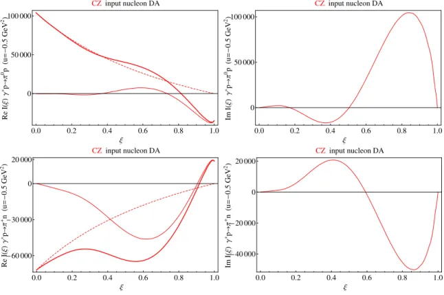
On Fig. 5 we present the results in our model for the real and imaginary parts of I(ξ) for backward production of π0 (two upper panels) and π+ (two lower panels) off proton
showing separately the spectral part, the pole part and their sum. The CZ phenomeno-logical solution [9] for the nucleon DA is used as the numerical input for our model. For
small ξ (ξ <∼ 0.3 ÷ 0.5), the real part is dominated by the contribution of the nucleon pole. The contribution of the spectral part to the real part becomes relatively more important for larger ξ. The nucleon pole contribution is purely real. The apparence of a significant imaginary part stemming from the spectral component of the model is a distinctive fea-ture of our approach. This is crucial for the non-vanishing of the transverse target single spin asymmetry for backward pion electroproduction discussed in Sec. 5.
0.0 0.2 0.4 0.6 0.8 1.0 0 50 000 100 000 Ξ Re IH Ξ L Γ *p ® Π 0p Hu = -0.5 GeV 2L CZ input nucleon DA 0.0 0.2 0.4 0.6 0.8 1.0 0 50 000 100 000 Ξ Im IH Ξ L Γ *p ® Π 0p Hu = -0.5 GeV 2L CZinput nucleon DA 0.0 0.2 0.4 0.6 0.8 1.0 -30 000 -60 000 0 20 000 Ξ Re IH Ξ L Γ *p ® Π +n Hu = -0.5 GeV 2L CZinput nucleon DA 0.0 0.2 0.4 0.6 0.8 1.0 -40 000 -20 000 0 20 000 Ξ Im IH Ξ L Γ *p ® Π +n Hu = -0.5 GeV 2L CZinput nucleon DA
FIG. 5: Real and imaginary parts of I(ξ) for γ∗p → π0p and γ∗p → π+n backward
production as functions of ξ computed in our two component model for πN TDAs. Dashed lines: nucleon pole contribution into ReI(ξ); thin solid line: spectral representation with input from the soft-pion theorem; solid line: sum of two contributions (for the real part).
5. UNPOLARIZED CROSS SECTION AND TRANSVERSE TARGET SINGLE
SPIN ASYMMETRY FOR BACKWARD PION PRODUCTION
Let us first specify our conventions for the backward pion electroproduction cross section. In the one photon exchange approximation, the unpolarized cross section of hard
leptoproduction of a pion off a nucleon (1) can be decomposed as follows [47]: d4σ dsdQ2dϕdt = αem(s − M2) 4(2π)2(kL 0)2M2Q2(1 − ε) ׳dσT dt + ε dσL dt + ε cos 2ϕ dσT T dt + p 2ε(1 + ε) cos ϕdσLT dt ´ , (47)
where ϕ is the angle between the leptonic and hadronic planes; s = (p1+ q)2 ≡ W2 and
t = (p2− p1)2 are the Mandelstam variables; kL0 is the initial state electron energy in the
laboratory (LAB) frame (beam energy). ε is the polarization parameter of the virtual photon: ε = h 1 + 2 ¡ kL 0 − k0L0 ¢2 + Q2 Q2 tan 2 θLe 2 i−1 , (48) where k0L
0 is the energy of the final state electron in the LAB frame and θLe is the electron
scattering angle in the LAB frame.
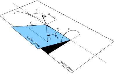
Within the suggested factorization mechanism for backward pion leptoproduction, only the transverse cross section dσTdt receives a contribution at the leading twist level. Using the explicit expression relating scattering amplitudes of leptoproduction to those for virtual photoproduction (eq. (2.12) of Ref. [47]), we express ddΩπ2σT in the center of mass (CMS) system of the pion and final nucleon through γ∗N → Nπ helicity amplitudes Mλ
s1s2 defined in (31): d5σ dE0dΩ e0dΩπ = Γ × Λ(s, m 2, M2) 128π2s(s − M2) X s1, s2 n1 2 ¡ |M1s1s2|2+ |M−1s1s2|2¢+ ... o = Γ ×³d 2σ T dΩπ + ... ´ . (49) Here, Ωe0 is the differential solid angle for the scattered electron in the LAB frame; Ωπ
is the differential solid angle of the produced pion in N0π CMS frame (see Fig. 6 for the
definition of angular variables); by dots, we denote the subleading twist terms supressed by powers of 1/Q; Λ is the usual Mandelstam function
Λ(x, y, z) = px2+ y2+ z2− 2xy − 2xz − 2yz. (50)
Γ is the virtual photon flux factor in Hand’s convention [48] given by Γ = αem 2π2 k0L 0 kL 0 s − M2 2MQ2 1 1 − ε. (51)
hadron plane lepton plane 0 ? ? e e s ∆ 1 pπ θπ p 1 ϕ ϕs
FIG. 6: Kinematics of electroproduction of a pion off a nucleon in the CMS frame of γ∗
nucleon.
Our present goal is to establish the expression for the LO transverse cross section through the helicity amplitudes defined in (34). We rewrite our formula (34) as
Ms1s2 λ = C 1 Q4U(p¯ 2, s2) ΓHU(p1, s1), (52) where ΓH = ˆ²(λ)γ5I − ˆ²(λ) ˆ ∆T M γ5I 0. (53)
Let us now square the amplitude and sum over the transverse polarizations of the virtual photon and over the spin of outgoing nucleon:
|Ms1 T |2 = |C|2 1 Q8 X λT Tr n (ˆp2+ M)ΓH 1 + γ5sˆ1 2 (ˆp1+ M)γ0Γ † Hγ0 o . (54)
Let us first consider the trace X λT Tr n (ˆp2+ M)ΓH(ˆp1+ M)γ0Γ†Hγ0 o = (55) −X λT ²ν(λ)²µ∗(λ)Trn(ˆp 2+ M) ¡ γνγ 5I − γν ˆ ∆T M γ5I 0¢(ˆp 1+ M) ¡ γ5γµI∗− γ5 ˆ ∆T M γ ν(I0)∗¢o.
We employ the relation X
²ν(λ)²µ∗(λ) = −gµν+ 1
(p · n)(p
to sum over the transverse polarizations of the virtual photon. We use the backward kinematics for the reaction (1) summarized in [10]:
p1· n = 1 + ξ 2 ; p1· p = M2 2(1 + ξ); p2· n = O(1/Q2); p2 · p = Q2 4ξ + O(Q 0). (57)
Then for the part which is independent of the nucleon spin we get: X λT Tr n (ˆp2+ M)ΓH(ˆp1+ M)γ0Γ†Hγ0 o = 2Q 2(1 + ξ) ξ |I| 2− 2Q2(1 + ξ) ξ ∆2 T M2|I 0|2+ O¡Q0¢ . (58)
Now we turn to the nucleon spin dependent part of the trace (54). X λT Tr n (ˆp2+ M)ΓHγ5sˆ1(ˆp1+ M)γ0Γ†Hγ0 o =X λT ²ν(λ)²µ∗(λ) n (ˆp2+ M)γνsˆ1(ˆp1+ M)γ5 ˆ ∆T M γ µoI(I0)∗ +X λT ²ν(λ)²µ∗(λ) n (ˆp2+ M)γν ˆ ∆T M sˆ1(ˆp1+ M)γ5γ µoI0(I)∗ = 4Q 2(1 + ξ) Mξ ε(n, p, s1, ∆T) ¡ − iI(I0)∗+ iI0(I)∗¢ = −4Q2(1 + ξ) ξ |∆T| M |~s1| sin(ϕ − ϕs)Im(I 0(I)∗). (59)
In the last line of (59), we consider s1 as being purely transverse and choose the reference
frame so that s1 has only an x-component. Then
ε(n, p, s1, ∆T) =
1
2|∆T||~s1| sin(ϕ − ϕs), (60)
where ϕ is the angle between the leptonic and hadronic planes and ϕsis the angle between
the leptonic plane the transverse target spin (see Fig. 6). We employ the conventions in which ε0123 = 1 with γ
5 = −4!iεµνρσγµγνγργσ . Finally, we conclude that
|Ms1 T |2 = |C|2 1 Q6 (1 + ξ) ξ µ |I|2− ∆2T M2|I 0|2− 2|∆T| M |~s1| Im(I 0(I)∗) sin ˜ϕ ¶ + O(1/Q8),(61) where ˜ϕ ≡ ϕ − ϕs.
Hence, we establish the following formula for the LO unpolarized cross section (49) through the coefficients I, I0, introduced in (34):
d2σ T dΩπ = |C|2 1 Q6 Λ(s, m2, M2) 128π2s(s − M2) 1 + ξ ξ ¡ |I|2 − ∆2T M2|I 0|2¢. (62)
Within our kinematics
∆2 T = (1 − ξ) ³ ∆2− 2ξ³M2 1+ξ − m2 1−ξ ´´ 1 + ξ , (63)
where m is the pion mass.
On Fig. 7, we present our estimates for the unpolarized cross section ddΩπ2σT (62) of backward production of π0 and π+ off protons for Q2 = 10GeV2 and u = −0.5GeV2 in
nb/sr as function of xB.
We use the two component model for πN TDAs presented in Secs. 3 and 4. In order to quantify the sensitivity of our model prediction on the input nucleon DAs, we show the cross section for the case of four phenomenological solutions fitting the nucleon elec-tromagnetic form factor: CZ [9] (solid lines), Chernyak-Ogloblin-Zhitnitsky (COZ) [41] (dotted lines), King and Sachrajda (KS) [42] (dashed lines), Gari and Stefanis (GS) [43] (dash-dotted lines) and Braun, Lenz and Wittmann next-to-next-to-leading order (BLW NNLO) [44, 45] . The magnitude of these cross sections is large enough for a detailed investigation to be carried at high luminosity experiments such as J-lab@12GeV and EIC. We recall that the scaling law for the cross section (62) is 1/Q8.
0.0 0.2 0.4 0.6 0.8 1.0 0.5 2.0 0.2 5.0 0.1 10.0 xB d 2 Σ T d WΠ @nb sr D Γ * p ® Π 0 p
CZv.s.COZv.s.KS v.sGSv.sBLW NNLOinput nucleon DA
0.0 0.2 0.4 0.6 0.8 0.50 0.10 0.05 0.01 xB d 2 Σ T d WΠ @nb sr D Γ * p ® Π + n
CZv.s.COZv.s.KSv.sGSv.sBLW NNLOinput nucleon DA
FIG. 7: Unpolarized cross section d2σT
dΩπ (in nb/sr) for backward γ∗p → pπ0 (upper panel)
and for backward γ∗p → nπ+ (lower panel) as the function of x
B computed in the two
component model for πN TDAs for Q2 = 10 GeV2, u = −0.5 GeV2 as a function of x B.
CZ [9] (solid lines), COZ [41] (dotted lines), KS [42] (short dashes), GS [43] (dash-dotted lines) and BLW NNLO [44, 45] (long dashes) nucleon DAs were used as inputs for our model.
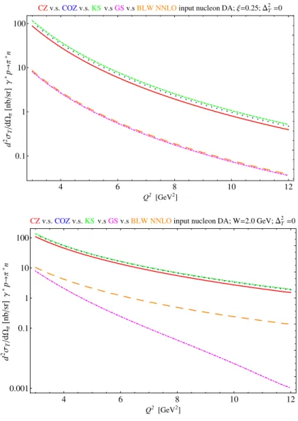
On the upper panel of Fig. 8, we show the Q2 dependence of the unpolarized
differ-ential cross section of γ∗p → nπ+ for fixed ξ = 0.25 which is characteristic for the J-lab
kinematics and for ∆2
T = 0. The plot exhibits the expected universal 1/Q8 scaling
behav-ior; the shape of πN TDAs, indeed, affects only the overall normalization. On the lower panel of Fig. 8, similarly to [51], we show instead the same cross section as the function
of Q2 for fixed W = 2.0 GeV and ∆2
T = 0. Let us emphasize that the scaling behavior
in the latter case is shadowed due to the fact that, for fixed W , the running of Q2 also
imposes variation of the scaling variable ξ.
4 6 8 10 12 0.1 1 10 100 Q2@GeV2D d 2Σ T d WΠ @nb sr D Γ *p ® Π +n
CZv.s.COZv.s.KSv.sGSv.sBLW NNLOinput nucleon DA; Ξ=0.25;DT2=0
4 6 8 10 12 0.001 0.1 1 10 100 Q2 @GeV2D d 2Σ T d WΠ @nb sr D Γ *p ® Π +n
CZv.s.COZv.s.KSv.sGSv.sBLW NNLOinput nucleon DA; W=2.0 GeV;DT 2
=0
FIG. 8: Upper panel: unpolarized cross section ddΩπ2σT (in nb/sr) for backward γ∗p → nπ+
for fixed ξ = 0.25 and ∆2
T = 0 as a function of Q2 in the two component model for πN
TDAs. Lower panel: unpolarized cross section d2σT
dΩπ (in nb/sr) for backward γ∗p → nπ+
for fixed W = 2.0 GeV and ∆2
T = 0 as a function of Q2 in the two component model
for πN TDAs. CZ [9] (solid lines), COZ [41] (dotted lines), KS [42] (short dashes), GS [43] (dash-dotted lines) and BLW NNLO [44, 45] (long dashes) nucleon DAs are used as inputs for the model.
Asymmetries, being ratios of the cross sections, are less sensitive to perturbative cor-rections. Therefore, they are usually considered to be more reliable to test the factorized description of hard reactions. For the backward pion electroproduction, an evident can-didate is the transverse target single spin asymmetry (STSA) [49] defined as:
A = 1 |~s1| µZ π 0 d ˜ϕ|Ms1 T |2− Z 2π π d ˜ϕ|Ms1 T |2 ¶ µZ 2π 0 d ˜ϕ|Ms1 T |2 ¶−1 = −4 π |∆T| M Im(I0(I)∗) |I|2− ∆2T M2|I0|2 . (64)
As argued in Sec. 4, within the two component model for πN TDAs, the non-vanishing of the numerator in the last equality of (64) is achieved due to the interference of the spectral part contribution into ImI(ξ) and of the nucleon pole part contribution into ReI0(ξ).
On Fig. 9, we show the result of our calculation of the STSA for backward π0 and π+
electroproduction off protons for Q2 = 10 GeV2 and u = −0.5 GeV2. CZ [9], COZ [41] ,
KS [42] and GS [43] nucleon DAs are used as phenomenological input for our model. We conclude that STSA turns out to be sizable in the valence region. Its measurement should therefore be considered as a crucial test of the applicability of our collinear factorized scheme for backward pion electroproduction.
0.0 0.2 0.4 0.6 0.8 1.0 -0.6 -0.4 -0.2 0.0 0.2 0.4 0.6 xB STSA Γ * p ® Π 0 p
CZv.s.COZv.s.KSv.sGS v.sBLW NNLOinput nucleon DA
0.0 0.2 0.4 0.6 0.8 1.0 -0.4 -0.2 0.0 0.2 xB STSA Γ *p ® Π +n H Q 2= 10 GeV 2, u = -0.5 GeV 2L
CZv.s.COZv.s.KSv.sGS v.sBLW NNLOinput nucleon DA
FIG. 9: Transverse target single spin asymmetry (64) for backward γ∗p↑ → pπ0 (upper
panel) and for backward γ∗p↑ → nπ+ (lower panel) as a function of x
B computed with
the two component model for πN TDAs for Q2 = 10 GeV2, u = −0.5 GeV2 as a function
of xB. We show the results of our model with different input nucleon DAs: CZ (solid
line), COZ (dotted line), KS (short dashes), GS (dot dashed line) and BLW NNLO (long dashes) used as input .
6. CONCLUSIONS
For the first time, we have managed to build a consistent model of πN TDAs in their whole domain of definition. It satisfies general constraints imposed by the underlying
QCD such as isospin symmetry, the Lorentz invariance manifested through the polynomi-ality property of the Mellin moments of πN TDAs in the light-cone momentum fractions, as well as the chiral properties. We used this model in the estimates of the unpolarized cross section and the transverse target single spin asymmetry for backward π+ and π0
electroproduction off protons. Our results make us hope for bright experimental prospects for measuring baryon to meson TDAs with high luminosity lepton beams such as COM-PASS, J-lab@ 12 GeV and EIC [50]. Experimental data from J-lab@ 6 GeV on backward
π+, π0, η and ω meson production are currently being analyzed [52]. We eagerly wait for
the first evidences of the factorized picture for backward electroproduction reactions as suggested in our approach.
Acknowledgements
We are thankful to Aurore Courtoy, Vladimir Braun, Michel Guidal, Valery Kubarovsky, C`edric Lorc`e, Kijun Park, Barbara Pasquini, Paul Stoler, Mark Strikman, Samuel Wallon and Christian Weiss for many discussions and helpful comments.
This work is supported in part by the Polish NCN grant DEC-2011/01/B/ST2/03915 and by the French-Polish Collaboration Agreement Polonium.
A. PARAMETRIZATION OF LEADING TWIST πN TDAS
The parametrization of the leading twist-3 πN TDAs of given flavor contents suggested in [12] which we employ in this paper reads:
4(P · n)3 Z "Y3 j=1 dλj 2π # eiP3k=1xkλk(P ·n)hπ(p π)| bOρ τ χ(λ1n, λ2n, λ3n)|N(p1)i = δ(x1+ x2+ x3− 2ξ) × i fN fπM £ VπN 1 (x1, x2, x3, ξ, ∆2)( ˆP C)ρ τ( ˆP U )χ +AπN 1 (x1, x2, x3, ξ, ∆2)( ˆP γ5C)ρ τ(γ5P U )ˆ χ+ T1πN(x1, x2, x3, ξ, ∆2)(σP µC)ρ τ(γµP U )ˆ χ +V2πN(x1, x2, x3, ξ, ∆2)( ˆP C)ρ τ( ˆ∆U)χ+ A2πN(x1, x2, x3, ξ, ∆2)( ˆP γ5C)ρ τ(γ5∆U)ˆ χ +T2πN(x1, x2, x3, ξ, ∆2)(σP µC)ρ τ(γµ∆U)ˆ χ+ 1 MT πN 3 (x1, x2, x3, ξ, ∆2)(σP ∆C)ρ τ( ˆP U )χ + 1 MT πN 4 (x1, x2, x3, ξ, ∆2)(σP ∆C)ρ τ( ˆ∆U)χ ¤ , (A1)
where fπ is the pion weak decay constant and fN is a constant, which determines the
value of the dimensional nucleon wave function at the origin; U is the usual Dirac spinor and C is the charge conjugation matrix. We employ Dirac’s “hat” notation: ˆa ≡ γµaµand
adopt the conventions: σµν = 1
2[γµ, γν]; σvν ≡ vµσµν, where vµ is an arbitrary 4-vector.
The relation of the parametrization (A1) for πN TDAs to that of [10] is given by:
{V1, A1, T1}πN ¯ ¯ [10] = µ 1 1 + ξ{V1, A1, T1} πN − 2ξ 1 + ξ{V2, A2, T2} πN¶ ¯¯¯
[12] & this paper;
{V2, A2}πN ¯ ¯ [10] = µ {V2, A2}πN+ 1 2{V1, A1} πN ¶¯¯ ¯ ¯
[12] & this paper
;
T3πN¯¯[10] = T2πN¯¯[12] & this paper+1 2 T
πN 1
¯ ¯
[12] & this paper
T2πN¯¯[10] = µ 1 2T πN 1 + T2πN + T3πN − 2ξT4πN ¶¯¯ ¯ ¯
[12] & this paper
; T4πN¯¯[10] = µ 1 + ξ 2 T πN 3 + (1 + ξ)T4πN ¶¯¯ ¯ ¯
[12] & this paper
. (A2)
B. AN ALTERNATIVE FORM OF SPECTRAL REPRESENTATION FOR
GPDS AND BARYON TO MESON TDAS
1. GPD in the ERBL and DGLAP regions
From (11), one can derive the following expressions for GPD in the DGLAP and the ERBL regions:
1. for −1 ≤ x ≤ −ξ (DGLAP 1 region):
H(x, ξ) = 1 1 − ξ Z 1−ξ+2x 1+ξ −1 dκF ³ κ,κ(1 + ξ) − 2x 1 − ξ ´ ; (B3)
2. For −ξ ≤ x ≤ ξ (ERBL region):
H(x, ξ) = 1 1 − ξ Z 1−ξ+2x 1+ξ −1+ξ+2x 1+ξ dκF ³ κ,κ(1 + ξ) − 2x 1 − ξ ´ ; (B4)
3. For ξ ≤ x ≤ 1 (DGLAP 2 region):
H(x, ξ) = 1 1 − ξ Z 1 −1+ξ+2x 1+ξ dκF³κ,κ(1 + ξ) − 2x 1 − ξ ´ . (B5)
2. Set of working formulas for πN TDAs in the ERBL-like and DGLAP-like regions
In order to be able to compute πN TDAs from the spectral representation (19), we perform integrals over µ and λ with the help of two δ-functions. We omit the index i referring to the choice of quark-diquark coordinates in the formulas of this Appendix.
The resulting domain of integration in (κ, θ) is defined by the inequalities:
−1 ≤ κ ≤ 1 ; −1 − κ 2 ≤ θ ≤ 1 − κ 2 ; −1 + ξ + 2w 1 + ξ ≤ κ ≤ 1 − ξ + 2w 1 + ξ ; κ 2 − 1 1 + ξ(w − 2v + 1 − ξ 2 ) ≤ θ ≤ − κ 2 + 1 1 + ξ(w + 2v + 1 − ξ 2 ). (B6)
Below, we summarize the explicit expressions for πN TDAs from the spectral repre-sentation (19) in the ERBL-like and DGLAP-like regions. Let us introduce the following notation for the integrand:
F (....) ≡ F µ κ, θ, κ(1 + ξ) − 2w 1 − ξ , θ(1 + ξ) − 2v 1 − ξ ¶ . (B7)
1. For w ∈ [−1; −ξ] and v ∈ [ξ0; 1 − ξ0+ ξ] (DGLAP-like type I domain):
H(w, v, ξ) = 1 (1 − ξ)2 Z 1−2v+w 1+ξ −1 dκ Z 1−κ 2 κ 2− 1 1+ξ(w−2v+ 1−ξ 2 ) dθF (....) (B8)
2. For w ∈ [−1; −ξ] and v ∈ [−ξ0; ξ0] (DGLAP-like type II domain):
H(w, v, ξ) = 1 (1 − ξ)2 Z 1−ξ+2w 1+ξ −1 dκ Z −κ 2+1+ξ1 (w+2v+ 1−ξ 2 ) κ 2− 1 1+ξ(w−2v+ 1−ξ 2 ) dθF (....) (B9)
3. For w ∈ [−1; −ξ] and v ∈ [−1 + ξ0− ξ; −ξ0] (DGLAP-like type I domain):
H(w, v, ξ) = 1 (1 − ξ)2 Z 1+2v+w 1+ξ −1 dκ Z −κ 2+1+ξ1 (w+2v+ 1−ξ 2 ) −1−κ 2 dθF (....). (B10)
4. For w ∈ [−ξ; ξ] and v ∈ [ξ0; 1 − ξ + ξ0] (DGLAP-like type II domain):
H(w, v, ξ) = 1 (1 − ξ)2 Z 1−2v+w 1+ξ −1+ξ+2w 1+ξ dκ Z 1−κ 2 κ 2− 1 1+ξ(w−2v+ 1−ξ 2 ) dθF (....). (B11)
5. For w ∈ [−ξ; ξ] and v ∈ [−ξ0; +ξ0] (ERBL-like domain): H(w, v, ξ) = 1 (1 − ξ)2 Z 1−ξ+2w 1+ξ −1+ξ+2w 1+ξ dκ Z −κ 2+1+ξ1 (w+2v+ 1−ξ 2 ) κ 2−1+ξ1 (w−2v+ 1−ξ 2 ) dθF (....).
6. For w ∈ [−ξ; ξ] and v ∈ [−1 + ξ − ξ0; −ξ0] (DGLAP-like type II domain):
H(w, v, ξ) = 1 (1 − ξ)2 Z 1+2v+w 1+ξ −1+ξ+2w 1+ξ dκ Z −κ 2+ 1 1+ξ(w+2v+ 1−ξ 2 ) −1−κ 2 dθF (....). (B12)
7. For w ∈ [ξ; 1] and v ∈ [−ξ0; 1−ξ +ξ0], the result coincides with (B11) as it certainly
should be, since this is the part of the same DGLAP-like type II domain. 8. For w ∈ [ξ; 1] and v ∈ [ξ0; −ξ0] (DGLAP-like type II domain):
H(w, v, ξ) = 1 (1 − ξ)2 Z 1 −1+ξ+2w 1+ξ dκ Z 1−κ 2 −1−κ 2 dθF (....). (B13)
9. For w ∈ [ξ; 1] and v ∈ [−1 + ξ − ξ0; ξ0], the result coincides with (B12), since this
is the part of the same DGLAP-like type II domain.
C. ON THE RELEVANT GENERALIZED FUNCTIONS
Sohotsky’s formula (see e.g. Chapter II of [40]) reads: 1
x ± i0 = ∓iπδ(x) + P
1
x, (C1)
where P stands for the Cauchy principal value prescription. The generalized function P 1 x2
is then defined as d
dxPx1 = −Px12. For an arbitrary test function ϕ(x),
µ P 1 x2, ϕ(x) ¶ = P Z dxϕ(x) − ϕ(0) x2 . (C2)
Employing (C1) and (C2) one can establish the familiar relation:
d dx 1 x ± i0 = ∓iπδ 0(x) − P 1 x2 . (C3)
The formula (C3) concerns the conventional generalized functions dealing with the class of test functions defined on (−∞; ∞) and sufficiently fast decreasing at the infinity. In our case, we have to consider a different class of generalized functions dealing with the
test functions defined on the interval [A; B] (A < 0, B > 0 so that the singularity point
x = 0 belongs to the interval). Let ϕ(x) be a test function defined on the interval [A; B].
Then Z B A µ d dx µ P1 x ¶ , ϕ(x) ¶ ≡ µ d dx µ P1 x ¶ , ϕ(x) ¶ [A, B] = 1 xϕ(x) ¯ ¯ ¯ ¯ x=B x=A − lim ²→0 µZ −² A + Z B ² ¶ dxϕ0(x) x . (C4)
Let us consider the integral term at the r.h.s of eq. (C4): lim ²→0 µZ −² A + Z B ² ¶ dxϕ 0(x) x = lim²→0 µZ −² A + Z B ² ¶ dx d dx(ϕ(x) − ϕ(0)) x = 1 x(ϕ(x) − ϕ(0)) ¯ ¯ ¯ ¯ x=B x=A + P Z B A dx1 x ϕ(x) − ϕ(0) x . (C5)
Thus we conclude that µ P 1 x2, ϕ(x) ¶ [A, B] ≡ − µ d dx µ P1 x ¶ , ϕ(x) ¶ [A, B] = − ϕ(0)1 x ¯ ¯ ¯ ¯ x=B x=A + P Z B A dx1 x ϕ(x) − ϕ(0) x . (C6) So finally we establish the following relation:
µ 1 (x ± i0)2, ϕ(x) ¶ [A,B] = ±iπ (δ0(x), ϕ(x)) [A,B]+ µ P 1 x2, ϕ(x) ¶ [A, B] = ∓iπϕ0(0) + ϕ(0)(B − A) AB + P Z B A dx1 x ϕ(x) − ϕ(0) x , (C7)
that represents the version of (C3) adopted for the use on the finite interval.
D. CALCULATION OF THE CONVOLUTION INTEGRALS
In the calculation of ReII(±,±)(ξ) and ReIII(−,±)(ξ), we encountered the following double principal value integrals
P Z 1 −1 dw 1 (w ± ξ)P Z 1−|ξ−ξ0| −1+|ξ−ξ0| dv 1 (v ± ξ0)H(w, v, ξ); (D1) P Z 1 −1 dw 1 (w − ξ)2P Z 1−|ξ−ξ0| −1+|ξ−ξ0| dv 1 (v ± ξ0)H(w, v, ξ). (D2)
We propose here a strategy of computation of these integrals once H(w, v, ξ) is param-eterized with the help of the spectral representation (19) with the use of the factorized Ansatz (20). The procedure generalizes the way of proceeding with the principal value integrals when computing the real part of the elementary DVCS amplitude with GPDs parameterized through Radyushkin’s factorized Ansatz. The following steps are to be performed:
1. By interchanging the order of integration in (D1) and (D2), w and v integrals may be computed using the two delta functions. One is left with four integrations over the spectral parameters.
2. After suitable change of variables, two principal value integrations can be performed analytically.
3. The double integration over the remaining two spectral parameters is performed numerically. The corresponding integrands possess only logarithmic singularities which are perfectly integrable. In this way, we managed to reduce the problem of performing highly singular principal value integrals (D1), (D2) to much less singular integration. This allows us to construct a stable and reliable numerical procedure. We present below the results for the principal value integral (D1) for the case of the factorized Ansatz (20) with the profile h(µ, λ), given by eq. (24).
P Z 1 −1 dw 1 (w ± ξ)P Z 1−|ξ−ξ0| −1+|ξ−ξ0| dv 1 (v ± ξ0)H(w, v, ξ) = 60η (±,±) (1 − ξ)5 Z 1 −1 dκ Z 1−κ 2 −1−κ2 dθ Z1 ¡ a(±,±)(κ, θ, ξ), b(±,±)(κ, θ, ξ), c(±)(κ, ξ)¢V (κ, θ). (D3) Here η is the sign factor:
η(±,+)= 1 ; η(±,−) = −1 . (D4)
The coefficient functions a(±,±), b(±,±) are defined as follows:
a(±,+)(κ, θ, ξ) = 1 2 µ 1 − κ 2 + θ ¶ (1 + ξ) ; a(±,−)(κ, θ, ξ) = 1 2 µ 1 − κ 2 − θ ¶ (1 + ξ) ; (D5)

![FIG. 2: Interpretation of πN TDAs within the light-cone quark model [16]. Small vertical arrows show the flow of the momentum](https://thumb-eu.123doks.com/thumbv2/123doknet/6439592.170921/4.892.120.773.473.851/interpretation-tdas-light-quark-small-vertical-arrows-momentum.webp)