Providing care for an elderly parent: interactions among siblings?

Providing care for an elderly parent: interactions among siblings?

Roméo FONTAINE*, Agnès GRAMAIN and Jérôme WITTWER

LEDa-LEGOS, Université Paris-Dauphine

January 2009

Abstract

This article is focused on children providing and financing long-term care for their elderly parent. The central aim of this work is to highlight the interactions that can appear between siblings when deciding whether or not to become a caregiver. We concentrate on families with two children using data from the Survey of Health, Ageing and Retirement in Europe (314 dependant elderly and their 628 adult children). In order to identify interactions between siblings, we have specified a two-person discrete game model. To allow us to estimate this model, without invoking the well-known "coherency" condition, we have added an endogenous selection rule to solve the incompleteness problem arising from multiplicity or absence of equilibrium. Our empirical results suggest that the three classical effects identified by Manski could potentially explain the observed correlation of caregiving behaviour among siblings. Correlated effects alone appear to be weak. Contextual interactions and endogenous interactions reveal cross-effects. The asymmetry of the endogenous interactions is our most striking result. The involvement of the younger child appears to increase the net benefit of caregiving for the elder child whereas the involvement of the elder child decreases the net benefit of caregiving for the younger child.

Keywords: Long-term care, Informal care, Social interactions, Discrete game model Classification JEL : C35, C72, D19, J14

*Correspondence to: Université Paris-Dauphine, LEDa-LEGOS, Roméo Fontaine, Place du Maréchal de Lattre de Tassigny 75775 Paris Cedex 16, France.

1. Introduction

It is without any doubt that informal care, in particular family care, is a crucial part of

long-term care. Any system of public aid for the elderly needs to be automatically linked with

informal care. For this reason, it is not only useful to examine the factors that contribute to

family involvement in caregiving, but also to measure to what extend formal caregiving and

informal caregiving are substitutes and to what extend public aid crowds out family support.

A reasonable amount of studies attempt to answer these questions, however their main focus

is not on care arrangement among siblings, that is, on the way siblings interact. This is for the

most part due to the authors’ assumption that caregiving is endured by a unique child,

generally the one who lives with the disabled, elderly parent. The present study loosens this

hypothesis and considers that several siblings may be involved in caring. Defining the

conditions which favour multiple informal caregiving, simultaneously establishes the

conditions which allow for the caregiving production burden to be divided among siblings.

Furthermore, from an academic point of view, it is particularly interesting to look at sibling

interaction in the event of a parental dependency within a family.

This paper is predominantly focused on the way in which siblings organize themselves to take

care of their aged, disabled parent living within the community. We try to understand the

interactions between siblings: does sibling involvement in parent support affect the

involvement of the other siblings? Can we assume that sibling involvements are independent?

If not, do we observe a negative or a positive link between sibling involvements? And finally,

Our interest is not in the arrangements taken for the care production among children who are

involved in caring. We ignore the type of caregiving and the intensity of caregiving provided

by each child caregiver and focus on what we call “care arrangement”: which children are

involved in caregiving, and which are not. Evidently, the decision for a sibling to participate

in caregiving is dependent on the expected caregiving production arrangement organised

between the involved siblings. A full comprehensive analysis would require a model that

incorporates the two decision moments (Pezzin et al., 2006). As we will see in more detail in

the following section, some authors have already proposed such comprehensive models.

Nevertheless, these structural approaches have confronted strong difficulties. First, it is very

challenging and complex to collect data that correctly and precisely represents the caregiving

production arrangement among siblings. Second, in order to feasibly manage these models,

the authors do not allow for care arrangements with multiple informal caregivers, which is

precisely the point we would like to investigate.

We prefer, thus, to adopt a direct model with the sole decision to participate in caregiving or

not. We assume that the child's utility is dependant on the actual decisions of his or her

siblings to participate or not in the caregiving and the observed care arrangement is assumed

to be a Nash equilibrium in this simple game.

Whatever the model adopted, a wide range of information is needed to analyse interactions

among siblings. The data should provide information on the aged as well as every family

member (at least each of his or her adult children). The SHARE survey (focused on people

aged 50 and above in 10 European countries) provides this type of data, even if little

information concerning the children is available. In this paper we have selected a sample of

dependant elderly1 (aged 65 and more), living without a spouse and having two adult children.

1

The participants are selected without a spouse, because our focus is on families with child

caregivers2. The selection requirement of two children is for simplicity and to neutralize a potential size effect (Fontaine et al., 2007).

Our paper proceeds as follows: Section 2 gives a brief overview of the analytical frameworks

used in the literature to model interactions between siblings during the decision to provide

care for an elderly parent, Section 3 and 4 describe our econometric model: preferences,

specifications, equilibrium conditions, and the outcome selection rule in the case of

indetermination, Section 5 describes the data used within this study, Section 6 reports the

main empirical results, and, finally, Section 7 concludes.

2. Analytical frameworks for modelling interaction between siblings

In our sample, care arrangements are distributed as follows : in four families out of ten (38%)

neither of the two children are caregivers, in roughly the same proportion (41%), one out of

two children are involved, and in two families out of ten both of the children are involved.

Shared caregiving among children is unexpectedly not insignificant. Furthermore, the

probability of a child to be involved in the caregiving of his or her dependant parent appears

to be higher when the other child is also involved than when it is not the case (50% and 34%

respectively). How can we explain these figures?

Naturally, our first response is to assume that the children’s decisions to give care are not

independent. Some studies (Bommier, 1995; Jellal and Wolff, 2002; Wolff, 2006) have tested

the independence of the children’s decisions using a direct estimation. In these studies, the

2 _{See Fontaine et al. (2007) for a more general analysis of family caregiving organisation in Europe and for a}

probability of each child to participate in caregiving production is a function of the

characteristics displayed by his or her sibling(s). This is a simple way to avoid the

endogeneity bias. The significant link between the probability of a child to participate and the

characteristics possessed by his or her sibling(s) cannot however be interpreted as evidence

for interdependence between the children’s decisions. Such a conclusion would be an

improper use of estimation results. It is indeed impossible a priori to disentangle what is

relevant to actual interactions from what is relevant to contextual effects or correlated effects

(Manski, 2000). For example, the gender of child 1 alone, independent of the child 1’s

caregiving decision, can influence the probability of child 2 to become the caregiver to their

aged parent. There are two main ways to bypass this difficulty. The first is to find an

instrumental variable linked to the decision of the sibling, but orthogonal to the decisions

made by the other siblings. In our context, this solution is clearly impracticable: any

measurable characteristic of a child which is assumed to influence his or her caregiving

decision is de facto a family characteristic. A second solution is to use a structural model of

the interactions.

Few studies have explored a structural approach. Two main options can be found in the

literature. Some studies (Checkovitch and Stern, 2002; Byrne et al. 2007), directly focused on

explaining care arrangements, that is which siblings are involved in the caregiving production,

consider the parent's well-being as a public good. Each child contributes knowing the

contribution of his or her siblings and the caregiving contribution of one child affects the

decision of the other children through the marginal productivity of their contribution. These

models appear too restrictive for our study because they assume that the decision to provide

care or to share the financial consequences of caregiving is exclusively based on productivity

that he or she does not have to take care of a dependant parent if his or her sibling is not

involved in the caregiving production. In this case, it is not a matter of caregiving

productivity, but solely a matter of what the child judges as a normal care arrangement (for

example a fair care arrangement).

In the second option of modelling, family caregiving organisation is viewed as the result of

two interaction steps: in the first step, each child decides whether to be involved in the family

decision or to draw back; in the second step, the caregiving organisation is collectively set up

by the involved siblings. Pezzin et al. (2006) developed this type of analytical framework and

defended the idea that, in the first step, interactions are non cooperative while, in the second

step, interactions have to be understood as cooperative interactions. Some studies (Engers and

Stern, 2002; Hiedemann and Stern, 1999) haveproposed to estimate this type of model. These

two step models can grasp the normative dimension of these children’s behaviours. For

instance, in the second step the cooperative caregiving production arrangement between the

involved children can indeed reveal the weight of each sibling in the collective decision.

Furthermore, in the first step, the links between the decision to participate of each child and

the probabilities to participate of his or her siblings may have normative interpretations.

Nevertheless, these models do not precisely consider the issue at stake for two reasons. First,

in the second step of these models, the family decision turns to the living arrangement for the

elderly parent but care arrangements where more than one child provides care usually do not

appear as a possible choice3. Second, the equilibrium concept used in the first step of these models do not allow for one child's decision to affect the decisions of the others. Indeed, the

authors use a Bayesian equilibrium solution which assumes that each child's decision depends

on the conjectures on sibling's behaviour and not on their actual behaviour. This

representation of interaction among siblings is not straightforward. It supposes that siblings

3 _{The choice set usually contains living alone in a separate household, living with one of the children}

play simultaneously and that each child decides to participate in caregiving production

without knowing the decision of their sibling(s). In the context of family interactions, this

representation appears to us quite unrealistic. It does not give any manner in which to

understand or interpret care arrangements as a result of interactions in the customary sense of

social interactions literature, in other words as a result of the reaction of each child to the

actual decisions of their siblings regarding participation in caregiving production.

Consequently, in order to test actual interactions among siblings without any a priori

assumption which could rule out potential normative motives and to be able to explain

multiple care arrangement, we have specified a very simple model which characterizes the

care arrangements through a stability condition with the following assumption of

non-cooperative interactions, each sibling decides whether to give care or not, knowing the

decision of the other (we only consider families with two children).By focusing the model on

involvement (as a binary variable) and studying two-child families, we get a two-person

discrete game model. The proposed model should be understood as a "semi-structural" model.

From a formal point of view and from a social interactions perspective these types of models

have the ability to avoid the reflexion problems described by Manski (2000). However, since

these models are written in terms of inequality restrictions, they also bring about the problem

of incompleteness4 (Tamer, 2003). However, using appropriate estimation methods allows us

to solve this incompleteness and to test how the observed behaviour of a child affects the

behaviour of his or her sibling.

4

3. Micro-econometric model

Already mentioned above, we only consider the case of two-child families. In a two-child

family j , the caregiving behaviour of a given child is represented by a binary variable a_ij

(i=1 for the elder child, i=2 for the younger child). a is equal to 1 if the child is involved _ij in caregiving (providing or financing care), 0 if not. In family j , four care arrangements

j

k are observable:

- None of the children are involved (a_1j =0 and a_2j =0): k_j =0 - The elder child is involved alone (a_1j =1and a_2j =0): k_j =1 - The younger child is involved alone (a1j =0 and a2j =1): kj =2

- Both of them are involved (a1j =1and a2j =1): kj =3.

To model the care arrangement, we assume that each child's decision whether to give care or

not is based on his or her utility maximisation. In order to be able to test the possibility of

interactions among siblings, the utility function of a child depends, not only on his or her own

involvement, but also on the behaviour of his or her sibling: U1j =U1j(a1j,a2j) and )

,

( 2 1

2

2j U j a j a j

U = . Therefore, a child can adopt a different behaviour depending on the

actual behaviour of his or her sibling.

No assumption is made regarding the mechanism that leads to a given care arrangement. We

assume only that the observed care arrangements are "stable". More precisely, neither child

wants to change their decision given the decision of the other child. We assume that the

Younger child

0 1

0 0;0 0;∆U_{2 j}(0)

Elder child

1 ∆U_{1 j}(0);0 ∆U_1j(1);∆U_2j(1)

The behaviour of a child depends on the net utility of caregiving, ∆Uij, i.e. the utility gap

between caregiving (aij =1) and no caregiving (aij =0). This gap varies according to the

behaviour of the other child.

) , 0 ( ) , 1 ( ) ( ) , 0 ( ) , 1 ( ) ( 1 2 1 2 1 2 2 1 2 1 2 1 j j j j j j j j j j j j a U a U a U a U a U a U − = ∆ − = ∆ (1)

Following, Brock and Durlauf (2001), Soetevent and Kooreman (2007), we assume that the

net benefit of caregiving is dependent on individual or family characteristics. It can be

additively decomposed into three components5:

. . ) ( . . ) ( 2 2 1 2 2 1 2 1 1 2 1 1 2 1 j j j j j j j j j j a X a U a X a U

ε

β

α

ε

β

α

+ + = ∆ + + = ∆ (2)

The first component, X_1j.α₁ (resp. X_2j.α ₂), is the structural component. It captures the

direct effect of a characteristic Xijk on the net benefit of caregiving (whatever the other child

may decide). This component is assumed to depend on 3 types of characteristics: i) the

individual characteristics: a child who is a non-worker may, for example, have a higher net

benefit of caregiving than one who is a worker, ii) the family context: i.e. the characteristics

of the disabled elderly parent and those of the other child. A child may have a higher net

5 _{Note that we allow the individual or family characteristics (}

j

X1 for the elder child, X2j for the younger child)

and the behaviour of the sibling to have a different impact on the net benefit of caregiving of the elder or

younger child, i.e. the coefficients α and β may be different for the elder and the younger child. As we will

see, our empirical results confirm the importance of this assumption as caregiving behaviours appear very different according to the birth rank of the child.

benefit of caregiving when the parent is severely disabled or a smaller one if the sibling is

retired, considering that the caregiving supply rests with him or her, iii) cross-effects between

the characteristics of each actor: for example, having a sister rather than a brother can

influence in different ways the net benefit of caregiving for man and woman. This component

should capture the contextual interactions and correlated effects due to observed variables.

The second component,a_2j.β₁ (resp. a_1j.β₂ ), is the interactional component. It measures the way the net benefit of caregiving is affected by the sibling's involvement. As specified, the

interactional component is reduced to a constant term. In this case, we constrain interactions

to be homogeneous across families. If this component is statistically significant

(

β

₁ ≠0 and

β

₂ ≠0 ) we will conclude that the behaviour of one child has an impact on the utility of the other and thus on his or her behaviour.

Lastly, the third component is the residual component. Some explanatory factors of the

decision to provide care or not are shared by the siblings, for example the characteristics of

the disabled parent. Some of these factors are captured by the explanatory variables of the

model, while others are most likely unobserved. In order to control for this potential bias of

endogeneity, we estimate the model allowing errors to be correlated within a family. We

assume that the residuals are distributed according to a bivariate normal density function:

(

ε_1j,ε_2j

)

~ N

[

0,0,1,1,ρ

]

, where ρ is the correlation coefficient between ε_1j and ε_2j. Therefore, a care arrangement (a1j,a2j)is a pure Nash equilibrium if:

) , 1 ( ) , ( ) , 1 ( ) , ( 1 2 2 1 2 2 2 1 1 2 1 1     − ≥ − ≥ j j j j j j j j j j j j a a U a a U a a U a a U (3)

As it is discussed in details below, for a given vector of exogenous variables (both observed

and unobserved), this definition of an equilibrium does not predict a unique value for the

family j a set of Nash equilibria, noted N , and to determine the probability for each care _j

arrangement to be a Nash equilibrium of N : _j

) 0 ) 1 ( 0 ) 1 ( ( ) 3 ( ) 0 ) 0 ( 0 ) 1 ( ( ) 2 ( ) 0 ) 1 ( 0 ) 0 ( ( ) 1 ( ) 0 ) 0 ( 0 ) 0 ( ( ) 0 ( 2 1 2 1 2 1 2 1 > ∆ ∩ > ∆ = ∈ > ∆ ∩ < ∆ = ∈ < ∆ ∩ > ∆ = ∈ < ∆ ∩ < ∆ = ∈ j j j j j j j j j j j j U U P N P U U P N P U U P N P U U P N P (4)

The issue now is to express from this specification the probabilities of the dependant variable

j

k .

4. Complete specification and estimation method

The specification (4) leads to an incomplete econometric model (Tamer, 2003; Maddala,

1983). The underlying economic model is well-defined and does not suffer from logical

inconsistency. However, it can generate multiple equilibria or no equilibrium; therefore, this

model is not able to provide the well-defined, reduced form needed for a derived econometric

model.

Two cases must be distinguished, each depending on the way the two children interact. First,

they can interact in a symmetric way: in case of positive (resp. negative) interactions, the two

children are subject to an increase (resp. decrease) in their probability of caregiving when the

sibling also is a caregiver. In this case, the symmetry of the interactions leads to either a single

equilibrium (Nj =

{ } { } { } { }

0 , 1 , 2 , 3 ) or multiple equilibria (Nj =

{ }

1,2 in the case of

negative interactions,

{ }

0,3 in the case of positive interactions). Second, interactions may be

asymmetric: one is subject to an increase in his or her probability of involvement when their

involvement when their sibling is involved. In this situation, the asymmetry of the interactions

leads to either a single equilibrium (N_j =

{ } { } { } { }

0 , 1 , 2 , 3 ) or no equilibrium (N_j =

{ }

ø ).

When using bivariate discrete game models, economists usually impose a "coherency"

condition (

β

₁.

β

₂ =0) in order to force the probability of the four outcomes to sum to one (Heckman, 1978). This would lead the model to always predict a unique outcome.

Unfortunately, this solution eliminates any simultaneity in the model. Another solution is to

characterise the equilibrium (at the family level) and to deal explicitly with the nonuniqueness

of the outcome. To solve this indetermination, we impose an equilibrium selection in the

region of nonuniqueness (Krauth, 2006), i.e. a function sel(k_j,N_j) which assigns a

probability to each care arrangement according to the set of pure Nash equilibria which are

consistent with the preference specification: sel(kj,Nj)≡P(kj /Nj).

To describe a well-defined probability distribution, the selection rule must obey the

constraints: 0 ) , (k_j N_j ≥ sel (5) 1 ) , ( and

∑

= j k j j N k sel (6)

The probability for a care arrangement to be selected which is not a pure Nash equilibrium is

assumed to be equal to 0:

{ }

ø and ∉ , ( , )=0 ≠

∀Nj kj Nj sel kj Nj (7)

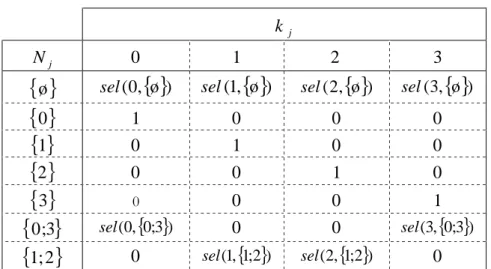
No other constraint was imposed a priori, so that the selection rule contains 5 free parameters

Table I: Selection rule:sel(k_j,N_j)

j

k

j

N 0 1 2 3

{ }

ø sel(0,

{ }

ø ) sel(1,

{ }

ø ) sel(2,

{ }

ø ) sel(3,

{ }

ø )

{ }

0 1 0 0 0

{ }

1 0 1 0 0

{ }

2 0 0 1 0

{ }

3 0 0 0 1

{ }

0;3 sel(0,

{ }

0;3) 0 0 sel(3,

{ }

0;3)

{ }

1;2 0 sel(1,

{ }

1;2) sel(2,

{ }

1;2) 0

with sel(0,

{ }

ø )+sel(1,

{ }

ø )+sel(2,

{ }

ø)+sel(3,

{ }

ø)=1 ,sel(1,

{ }

1;2)+sel(2,

{ }

1;2)=1 and sel(0,

{ }

0;3)+sel(3,

{ }

0;3)=1

Given the selection rule (table I), the probabilities of observing each care arrangement

according to the different sets of pure Nash equilibrium are6:

{ }

{ }

{ }

{ }

{ }

{ }

{ }

{ }

{ }

{ }

{ }

{ }

{ }

{ }

{ }

{ }

3 ) (3,

{ }

0;3). (

{ }

0;3 ) (3,

{ }

ø ). (

{ }

ø ) ( ) 3 ( ) ø ( . ) ø , 2 ( ) 2 ; 1 ( ). 2 ; 1 , 2 ( ) 2 ( ) 2 ( ) ø ( . ) ø , 1 ( ) 2 ; 1 ( . ) 2 ; 1 , 1 ( ) 1 ( ) 1 ( ) ø ( ). ø , 0 ( ) 3 ; 0 ( . ) 3 ; 0 , 0 ( ) 0 ( ) 0 ( = + = + = = = = + = + = = = = + = + = = = = + = + = = = j j j j j j j j j j j j j j j j N P sel N P sel N P k P N P sel N P sel N P k P N P sel N P sel N P k P N P sel N P sel N P k P (8)

In order to estimate the model with the maximum likelihood method, we need to express the

probability of observing each care arrangement as a function of the exogenous variables. First,

we then express the probability of each sets of pure Nash equilibrium according to the

probability that each care arrangement be a Nash equilibrium:

6 _{Note that according to the sign of the interactions, some sets of pure Nash equilibrium are unobservable.}

- When β₁>0 and β₂ >0 :P(N_j =

{ }

0;3 )>0 ,P(N_j =

{ }

1;2 )=0,P(N_j =

{ }

ø )=0. - When β1<0 and β2 <0:P(Nj =

{ }

0;3 )=0 ,P(Nj =

{ }

1;2 )>0,P(Nj =

{ }

ø )=0.

{ }

{ }

{ }

{ }

{ }

{ }

{ }

{ }

{ }

[

]

{ }

[

]

{ }

ø ) .

[

1 (0 ) (1 ) (2 ) (3 )

]

( 1 ) 3 ( ) 2 ( ) 1 ( ) 0 ( . ) 3 ; 0 ( 1 ) 3 ( ) 2 ( ) 1 ( ) 0 ( . ) 2 ; 1 ( ) 3 ; 0 ( ) 3 ( ) 3 ( ) 2 ; 1 ( ) 2 ( ) 2 ( ) 2 ; 1 ( ) 1 ( ) 1 ( ) 3 ; 0 ( ) 0 ( ) 0 ( 0 . 0 , 0 0 , 0 2 1 2 1 2 1 j j j j j j j j j j j j j j j j j j j j j j j j j j j N P N P N P N P I N P N P N P N P N P I N P N P N P N P N P I N P N P N P N P N P N P N P N P N P N P N P N P N P ∈ − ∈ − ∈ − ∈ − = = − ∈ + ∈ + ∈ + ∈ = = − ∈ + ∈ + ∈ + ∈ = = = − ∈ = = = − ∈ = = = − ∈ = = = − ∈ = = < > > < < β β β β β β (9)

where Iβ₁<0,β₂<0 =1 if interactions are symmetric and negative, 0 elsewhere; 1 0 , 0 2 1> β> = β

I , if interactions are symmetric and positive, 0 elsewhere; _{. 0} 1

2 1β < =

β

I , if

interactions are asymmetric, 0 elsewhere7.

Subsequently, with regard to the specification of net benefit of caregiving (4), the

probabilities that a care arrangement be a pure Nash equilibrium can be rewritten as function

of the exogenous variables:

) , , ( ) 3 ( ) , , ( ) 2 ( ) , , ( ) 1 ( ) , , ( ) 0 ( 2 2 2 1 1 1 2 2 1 1 1 2 2 2 1 1 2 2 1 1

ρ

β

α

β

α

ρ

α

β

α

ρ

β

α

α

ρ

α

α

+ + = ∈ − − − = ∈ − − − = ∈ − − = ∈ j j j j j j j j j j j j X X F N P X X F N P X X F N P X X F N P (10)

where F is the joint cumulative distribution of the bivariate normal.

Given the systems of equation (8), (9) and (10), we can finally express the probabilities of

each outcome as a function of the exogenous variables and parameters

α

1,

α

2,

β

1,

β

2,

ρ

,

) , (k_j N_j

sel .

For a given value of the selection rule’s parameters, the parameters of the utility function can

be estimated with the maximum likelihood criteria (using STATA). Conversely, for a given

7

The presence of these three dummies indicates that the likelihood function is non-differentiable at the points 0

ˆ

1=

estimation of the utility function parameters, we can get an approximation of the selection

rule’s parameters: the proportion of observed care arrangements conditional on the set of

Nash equilibria simulated for each family with the estimated utility functions. We exploit this

through an iterative strategy: at first step, we adopted an arbitrary set of values for the

selection rule (the equi-probability of each possible care arrangement), and estimated the

parameters of the utility function by likelihood maximisation. It allows us to simulate the set

of Nash equilibria for each family and to get an approximation for the selection rule’s

parameters, based on these first-step estimations. A second step of estimation is run, using the

“updated” values for the selection rule and so on. The process is repeated until the selection

rule’s parameters converge. The convergence is actually very fast, never more than four

iterations. This strategy has the advantage to improve the likelihood of the model, compared

to an arbitrary selection rule selected a priori as it is usually done in the literature8.

5. The data: SHARE

For the estimation of this model, we use the 2004 wave of the Survey of Health, Ageing and

Retirement in Europe database. It is a multidisciplinary and cross-national database of micro

data on health, socio-economic status and social and family networks of more than 27,000

individuals aged 50 or over. Data collected include health variables (e.g. self-reported health,

health conditions, physical and cognitive functioning, health behaviour, use of health care

facilities), bio-markers (e.g. grip strength, body-mass index, peak flow), psychological

variables (e.g. psychological health, well-being, life satisfaction), economic variables (current

work activity, job characteristics, opportunities to work past retirement age, sources and

composition of current income, wealth and consumption, housing, education), and social

8 _{Tamer (2003) states that ad hoc choices of a selection rule may lead to inconsistent estimates. However,}

simulations proposed by Krauth (2006) show that a misspecification of the selection rule has minimal effect on the resulting parameter estimates.

support variables (e.g. caregiving within families, transfers of income and assets, social

networks, volunteer activities) (Börsch-Supan et al., 2005).

For the sake of homogeneity, we reduce the sample to a population aged 65 or over, reporting

at least one limitation in activities of daily living (ADL) or instrumental activities of daily

living (IADL), and living without a spouse while having two children. Our sample contains

314 elderly and their 628 children.

The dependant variable of the model is the family’s care arrangement (a1j, a2j). We defined as

caregiver any child living with their disabled elderly parent or living apart but financing9 or providing help in kind (personal care, practical household help or help with paper). Such a

broad definition of involvement allows us to lessen the well-known impacts of the disability

level or of the political framework (supply side effects, solvabilisation…) on informal care10

in order to emphasize other effects such as interactions. However it creates a deterministic

relationship between the child’s location and the dependant variable so that the children’s

location could not be used as exogenous variable anymore11.

Each child’s decision is assumed to depend on three groups of variables, through the

structural component of the utility function (appendix B). In the first, we control for

individual effects: gender, age, education level, marital status and employment. Other factors,

as the child health status or the child income, may explain the caregiving decision but they are

not available in SHARE. The second and third groups of variables describe the context of the

9 _{Very few children provide financial care (5%) and 72% of them provide also help in kind (only 1% provide}

financial help without providing help in kind).

10

The way children provide care to their elderly parents varies across Europe, intergenerational household being more common in the south for example. But aggregating the different ways of caregiving leads to amazing regularities (see Fontaine et al., 2007).

11 _{The fact that location could be endogenous was examined by Stern, 1995 or Konrad & Robledo, 2002 for}

decision. We include information on the parent: gender, age, disability level, income, wealth

(we used a variable indicating if the parent is "sure" or not to have more than 50 000 euros at

the time of his or her decease) and education level. Using the distinction proposed by Manski

(Manski, 2000) these variables capture "correlated effects" in the behaviour of the children, as

part of the context is the same for both of the children of a given family. For each child, the

utility gap between caring and not caring is also assumed to depend directly on his or her

brother's or sister's characteristics (using the same variables as for individual effects). These

variables refer to "contextual interactions" (Manski, 2000).

6. Results

We estimated several versions of the model described in sections 3 and 4. We first estimate a

model allowing to correlated residuals12. The estimated correlation coefficient is equal to -0,251 but it is not significant. In order to test the effect of the selection rule we also estimated

the model with two ad hoc selection rules (equal probabilities for each possible care

arrangement13 ; systematic selection of the care arrangement without any informal care when

no Nash equilibrium exists). Table V (appendix C) reports the estimation of the endogenous

interactions parameters with each one of these selection rules. Estimation results are very

similar – the sign, size and significance of estimates remain the same – except for the

interaction parameters of the younger children which loose significance under some

specifications. The results reported here, in table II, were obtained with uncorrelated residuals

and an endogenous selection rule. Model 1 assumes that interactions are homogeneous across

families (

β

1and

β

2 are constants). Since we can also suppose that, beyond the birth rank, the

sign and the size of the interactions vary across families, we estimate a second model (model

12 _{To preserve space, estimation results are not shown. They are available on request.}

13 _{Bjorn and Vuong (1984), Kooreman (1994) or Soetevent and Kooreman (2007) consider the same selection}

214), in which the interactional component of the utility functions may vary according to some individual and family characteristics (V ): _ij

j j j j j j j j j j j j V a X a U V a X a U 2 2 2 1 2 2 1 2 1 1 1 2 1 1 2 1 . . . ) ( . . . ) (

ε

β

α

ε

β

α

+ + = ∆ + + = ∆ (11)

6.1. Parameters of the utility function

The coefficient estimates suggest that correlated effects are weak. Only the parent’s age

affects both of the children (in model 1, the coefficient estimate associated with parent's age

"under 75" is -0.78 for the elder child and -0.73 for the younger). With the exception of the

age effect, the elder child’s behaviour is not influenced by the characteristics of his parent,

whereas the younger children’s behaviour is much more dependent on the parent’s

characteristics: they have a lower net benefit of caregiving when the disabled parent is a man,

when he or she has not completed secondary school and when he or she has a low income.

Two set of variables, the country dummies and the parent disability, are not significant. This

result could be partly explained by the definition used here for individual involvement in

caregiving production: ignoring the type and the intensity of caregiving leads to more

homogeneous behaviours between European countries and between those having a severely

dependant parent and those having a slightly dependant parent (Fontaine et al., 2007).

As regards "contextual interactions", the most striking result is that the sibling's characteristics

are much more significant when they are measured relative to those of the other child, except

for employment status. The net benefit of caregiving is better explained by the age and

education gap than by the absolute age and education level. Furthermore, having a brother

does not have the same impact for men and women: having a brother raises the net benefit of

14 _{A version of model 2 allowing for correlated residuals has also been estimated but residuals appear}

caregiving of daughters (the coefficient estimate is 0.43 for elder daughters and 0.32 for

younger daughters), but it has no effect on elder sons and decreases the net benefit of

caregiving of younger son’s (the estimate coefficient is -0.53).

Turning now to the interactional component of the net benefit equation, estimation results

confirm that the child's behaviour is affected by their sibling's involvement in caregiving.

More unexpected, however, are the signs of the coefficients: the coefficient estimate in model

1 is positive for the elder children (

β

ˆ1=1.09) and negative for the younger (

β

ˆ2=−0.72).

Thus, our results reveal an asymmetry between elder and younger children in the way their

involvement is affected by the sibling's involvement: on average, the involvement of the

younger child increases the elder child’s net benefit of caregiving (positive interactions)

whereas the involvement of the elder child decreases the younger child’s net benefit of

caregiving (negative interactions)15,16.

15 _{Due to the non-differentiability of the likelihood function at point 0, 0}

2 1= β =

β , it is not possible to carry on

usual tests for testing the significance of endogenous interactions. A solution is to restrict the support of the

parameters to

]

−∞;0

]

or

[ [

0;∞ . In this case, the distribution of the test statistic is affected by the fact that tested

values are on the boundary (Gouriéroux C, Holly A and Monfort A., 1982; Andrews, 2001). We tested

“β₁=0,β₂ =0” against “β₁f0or β₂ p0 ” using the likelihood ratio. The distribution of the statistic is

dominated by a Chi2 with 2 degrees of freedom. The value of the statistics is 13.48 so that we can reject the null hypothesis with an error probability lower than 0.01.

16_{As Krauth (2006), we compare these results with those obtained from two independent probit models, one}

modelling the elder’s involvement (with the younger’s involvement as explanatory variable) and one modelling the younger’s involvement (with the elder’s involvement as explanatory variable). The endogenous interactions obtained from these two probit model are: βˆ_1,Probit=0.47(Pvalue=0.003) and βˆ_2,Probit=0.22 (Pvalue=0.178). Because

of the negative correlation between the younger’s involvement and the error term, the probit model

underestimate the true effect β₁. On the contrary, because of the positive correlation between the elder’s

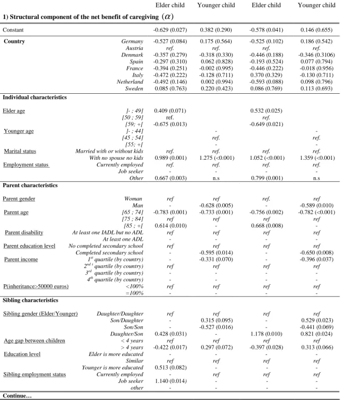
Table II: Estimated coefficients

Model 1

(homogeneous interactions)

Model 2

(heterogeneous interactions)

Elder child Younger child Elder child Younger child

1) Structural component of the net benefit of caregiving (α)

Constant -0.629 (0.027) 0.382 (0.290) -0.578 (0.041) 0.146 (0.655) Country Germany Austria Denmark Spain France Italy Netherland Sweden -0.527 (0.084) ref. -0.357 (0.279) -0.297 (0.310) -0.394 (0.251) -0.472 (0.222) -0.492 (0.146) 0.085 (0.763) 0.175 (0.564) ref. -0.318 (0.330) 0.062 (0.828) -0.002 (0.995) -0.128 (0.711) 0.002 (0.994) 0.220 (0.423) -0.525 (0.102) ref. -0.446 (0.188) -0.193 (0.524) -0.446 (0.222) 0.370 (0.329) -0.593 (0.088) 0.086 (0.769) 0.186 (0.542) ref. -0.346 (0.3106) 0.077 (0.794) -0.018 (0.956) -0.130 (0.711) 0.098 (0.796) 0.113 (0.693) Individual characteristics Elder age ]- ; 49] [50 ; 59] [59; +[ Younger age ]- ; 44] [45 ; 54] [55; +[

Marital status Married with or without kids

With no spouse no kids

Employment status Currently employed

Job seeker Other 0.409 (0.071) ref. -0.675 (0.013) ref. 0.989 (0.001) ref. - 0.667 (0.003) - ref. - ref. 1.275 (<0.001) ref. - n.s 0.532 (0.025) ref. -0.649 (0.021) ref. 1.052 (<0.001) ref. - 0.799 (0.001) - ref. - ref. 1.359 (<0.001) ref. - n.s Parent characteristics

Parent gender Woman

Man

Parent age [65 ; 74]

[75 ; 84] [85 ; +[

Parent disability At least one IADL but no ADL

At least one ADL

Parent education level No completed secondary school

Completed secondary school

Parent income 1st _{quartile (by country)} 2ndt _{quartile (by country)} 3rd _{quartile (by country)} 4th _{quartile (by country)}

P(inheritance>50000 euros) <100% =100% ref - -0.783 (0.001) ref 0.614 (0.010) ref - ref - - ref - - ref - ref -0.628 (0.005) -0.733 (0.001) ref - ref - ref -0.595 (0.014) -0.331 (0.070) ref - - ref - ref. - -0.756 (0.002) ref 0.668 (0.008) ref - ref - - ref - - ref - ref -0.589 (0.010) -0.782 (<0.001) ref - ref - ref -0.650 (0.008) -0.396 (0.037) ref - - ref - Sibling characteristics

Sibling gender (Elder/Younger) Daughter/Daughter

Son/Daughter Son/Son Daughter/Son

Age gap between children < 4 years

> 4 years

Education level Elder is more educated

Similar Younger is more educated

Sibling employment status Currently employed

Job seeker other ref - - 0.428 (0.031) ref -0.422 (0.017) - ref 0.513 (0.082) - 1.140 (0.014) - ref 0.315 (0.095) -0.527 (0.016) - ref 0.297 (0.072) - ref - ref - - ref - - 1.178 (0.010) ref -0.397 (0.028) - ref - ref - - ref 0.529 (0.023) -0.441 (0.069) 0.821 (0.024) ref 0.313 (0.066) - ref - ref - - Continue…

Continue…

Model 1 Model 2

Elder child Younger child Elder child Younger child

2) Interactional component of the net benefit of caregiving (β)

Constant 1.089 * -0.718 * 1.081 (0.001) -0.226 (0.462) Sibling gender (Elder/Younger) Daughter/Daughter

Son/Daughter Son/Son Daughter/Son

Education level Elder is more educated

Similar Younger is more educated

Parent income 1stt _{quartile (by country)} 2ndt _{quartile (by country)} 3rd _{quartile (by country)} 4th _{quartile (by country)}

Sibling employment status Currently employed

Job seeker or other

ref - - 0.813 (0.058) - ref 1.489 (0.046) - ref - -0.958 (0.010) ref -0.742 (0.021) ref - - -1.263 (0.016) -1.550 (0.044) ref - - ref - - ref - Log likelihood - 346.418 -336.219

P-value are given in parentheses

Note : The size of our sample (N=314) force us to be the as parsimonious as possible in the choice of explanatory variables. We then estimate an unrestricted model excluding, by backward elimination, the insignificant variables. Only the country dummies have been retained even if they are insignificant. Results presented here are those obtained after exclusion of variables which are statistically insignificant at the 10% level.

* due to the nondifferentiability of the likelihood function, the usual Wald statistic can not be used for testing )

0 and 0

(β₁ = β₂ = . Considering restricted support for these parameters β₂∈

]

−∞;0

]

and β₁∈

[ [

0;∞ , we can

use the likelihood ratio, but the distribution of the statistic is then a mixture of Chi2 (0) to Chi2(2), which is dominated by the distribution of a Chi2(2).

Restriction Restricted loglikelihood

) 0 and 0 (β₁ = β₂ = -353.16 ) 0 (β₁ = -352.16 ) 0 (β₂ = -348.82

6.2. The two effects of interactions

The existence of interactions has two effects on the care arrangement effectively set up in a

family. (i) It modifies the probabilities that a given care arrangement is a Nash equilibrium. In

the elder’s behaviour should lead to a lower proportion of families in which the younger child

provides care alone and a higher proportion of families in which the children give care to the

parent together. Inversely, the younger child’s behaviour should lead to a higher proportion

of families in which the elder child provides care alone and a lower proportion of families in

which the children both give care to the parent. The overall effect of interactions on the

probability of observing care arrangements with multiple caregivers is thus a priori

indeterminate. (ii) The simultaneity and the asymmetry of the interactions lead some families

to a situation without equilibrium: on average, the estimated probability that no equilibrium

exists is 7%17. In this case, the observed care arrangement results from the selection rule. When there is no equilibrium, the selection rule estimated with model 1 predicts that none of

the children are caregivers with a probability of 36%; only the elder child is a caregiver with a

probability of 22%; only the younger child is a caregiver with a probability of 22% and both

of them are caregivers with a probability of 21%.

In order to evaluate quantitatively the effect of the interactions, we simulated for each family

within the sample the probabilities of each care arrangement obtained with interactions and

those obtained without interaction, i.e. if the sibling behaviours were independent (

β

₁ =0 and

0

2 =

β

). Table III proposes a comparison of the average effects obtained in the sample.

Controlling for contextual interactions and correlated effects, the positive interactions

characterizing the elder child leads to a reduction of 0.18 of the probability that the younger

child gives care alone18. On the other hand, the negative interaction characterizing the

younger child leads to a 0.07 increase in the probability that the elder child gives care alone.

17 _{It is important to note that through this second effect alone, interactions modify the probability that the parent}

does not receive care from his or her children. The probability that the care arrangement without a caregiver is a Nash equilibrium is not directly influenced by the existence of interactions, as interactions only play a role in families where at least one child is involved in the caregiving provision.

18 _{Note that our comments do not take in account the effect produced by situations without equilibrium and their}

Furthermore, taking into account the existence of interactions, children are on average more

likely (0.04) to share the provision of caregiving. On average, the reaction of the elder child,

which allows us to explain the positive correlation observed between the decisions of the

children of a same family, is not entirely compensated by the negative interactions

characterizing the younger child.

Table III: Mean simulated effect of interactions (simulated with themodel 1)

) 1 ( Without interactions 0 1= β 0 2 = β ) 2 ( With interactions 089 . 1 1 = β 718 . 0 2 =− β Effect of interactions ) 1 ( ) 2 ( −

Probabilities of each Nash set

P(N_j =

{ }

0 ) 0.35 0.35 0 P(Nj =

{ }

1 ) 0.13 0.20 0.07 P(Nj =

{ }

2 ) 0.36 0.18 -0.18

{ }

3 ) (N_j = P 0.16 0.20 0.04

{ }

ø ) (N_j = P 0 0.07 0.07

Probabilities of each care arrangement

P(k_j =0) 0.35 0.38 0.03 P(k_j =1) 0.13 0.21 0.08 ) 2 (kj = P 0.36 0.20 -0.16 ) 3 (k_j = P 0.16 0.21 0.05

Note: For each family we simulated, with model 1, the probabilities of each Nash set and the probabilities of observing each care arrangement. Results presented here give the mean probabilities in the sample.

However, as the interaction effect is highly non-linear, the mean interaction effect gives only

a partial picture of the true effect. The overall effect of asymmetric interactions on the

probability of observing care arrangements with multiple caregivers is in fact positive for 73%

of the families of the sample, but negative or null for 27%.

To give an illustration let us consider two extreme cases present in our sample. First, consider

son. In this family, the elder daughter has a high net benefit of caregiving, even if her younger

brother is not involved. On the contrary, the younger son of this family has a slightly positive

net benefit of caregiving when his sister is not involved, but a negative net benefit of

caregiving when she is. His behaviour is thus highly dependent on his sister’s behaviour:

when his sister is involved he prefers not to provide care, whereas when she is not he prefers

to provide care. In this family, given the weakness of the positive marginal effect of the

younger son’s involvement on the elder daughter’s probability to provide care and the

significant negative marginal effect of the elder daughter’s involvement on the younger son’s

probability to provide care, interactions within this family reduces the probability that the

provision of care is shared between siblings by 19%. Consider now family B, composed of a

parent aged 85 or over, an elder son aged 60 or over and a younger daughter living alone.

Entirely opposite to family A, here, the elder son has a slightly negative net benefit of

caregiving when his sister is not involved, but a positive net benefit of caregiving when she is.

His behaviour is thus highly dependent on his sister’s behaviour. The younger daughter, given

her characteristics, has a high net benefit of caregiving, even if her brother is involved. In this

family, interactions increase the probability that the provision of care is shared among siblings

by 35%.

6.3 Variables affecting the sign and size of interactions

Estimation results for model 2 (table II) show that the negative interactions that characterize

younger children in model 1 are due to specific types of younger children : except for men

having a sister and children whose elder is more educated, the involvement of younger

children seems in fact to be independent of the elder children’s involvement.

Social characteristics, such as gender and education level, appear to be one of the main

the effect of sibling involvement on the net benefit of caregiving is of greater importance in

families composed of an elder daughter and a younger son. Regarding the effect of education

level, any difference in educational levels among siblings seems to reinforce the asymmetry in

the interactions: when the younger child is more educated (than the elder), his or her

involvement in caregiving increases the net benefit of caregiving of the elder, whereas, when

the elder is more educated (than the younger) his or her involvement decreases the net benefit

of caregiving of the younger.

These results can clearly receive different interpretations but the normative motive seems

quite relevant for these social effects: the duty to give care to an elderly parent seems to lie

more heavily upon the elder child than on the younger child and this would be all the more

prominent when the elder is female and the younger is male or when the elder is less

educated.

In contrast to social determinants, economic considerations seem to induce homogeneity in

the net benefit functions. For instance, the increase in the elder’s probability to provide care

induced by the involvement of the younger child is smaller when the younger child does not

work or when their parent is well-off. This result could reflect a sort of collective economic

principle, as if economic considerations could counteract the assignment of sibling role

according to birth order: when the time-constraint faced by the younger child is weak or when

a high income enables the parent to purchase formal care, it is easier for the elder child to

withdraw from assisting the younger child in providing care. We reach at this point one limit

of our semi-structural model which does not model the care production and its intensity. It is

indeed likely that the previous result is due to the fact that when the involved younger child

does not work, the care production is often large which is comforting for the not involved

7. Conclusion

Our empirical results suggest that the three classical effects distinguished by Manski can

indeed explain the observed correlation of caregiving behaviour among siblings. However,

correlated effects appear to be weak for multiple reasons. First, the characteristics of the

shared context that affect the child's net benefit of caregiving differ for the elder child

compared to the younger child. Second, we cannot reject the hypothesis of independence of

the residuals within the families. As regards "contextual interactions", it appears that sibling

characteristics are generally considerably more significant when they are measured relative to

those of the child. For example, the net benefit of caregiving is better explained by age and

education gap than by absolute age and education level. Endogeneous interactions seem

relevant, but our results reveal cross-effects between endogenous interactions, on the one

hand, and contextual effects and correlated effects, on the other hand. The caregiving decision

of one child affects directly the net benefit of caregiving of the other child, but its effect

depends on the parent and sibling characteristics. Our most unexpected result is the

asymmetry of endogenous interactions: the involvement of the younger child appears to

increase the net benefit of caregiving of the elder one, whereas the involvement of the elder

child decreases the net benefit of caregiving of the younger one. Social characteristics seem to

encourage asymmetry, most probably driven by normative motives. Our results can reflect

different expectations in terms of filial duty, according to the birth rank and the gender of

each child. Inversely, economic considerations appear to make the reaction to sibling’s

involvement by the elder and the younger child more symmetric. For example, when the

younger child faces more flexible constraints, the elder child’s net benefit of caregiving

becomes less dependent on the decision of the other child. The better economic conditions of

Appendix A

Indetermination of the econometric model

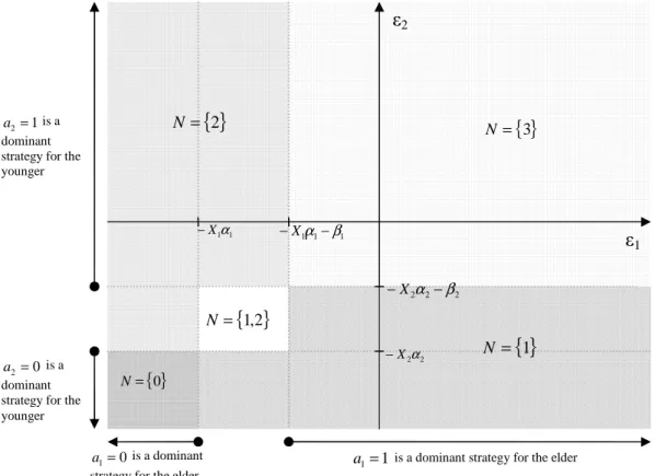
For a given vector of characteristics (observed and unobserved) it is possible to determine the

set of Nash-equilibria. Three cases are distinguished here. The results for the case of

symmetric and negative interactions are reported in figure 1. In this case, both children are

subject to a decrease in their net benefit of caring, when the other is involved in caregiving.

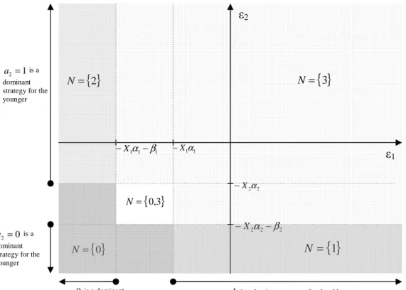
The case of symmetric, but positive interactions is reported in figure 2 (both children are

subject to an increase in their net benefit of caregiving, when the other is involved in

caregiving). Figure 3 applies when the elder is subject to positive interactions while the

younger is subject to negative interactions (estimation results for model 1 correspond to this

case). In each case, the indetermination region appears in white.

Figure 1: Nash equilibria when

β

₁ <0and

β

₂ <0

ε₁ ε₂ 1 1 1α −β −X

{ }

3 = N

{ }

2 = N

{ }

1 = N

{ }

1,2 = N { }0 = N 2 2 2α −β −X 2 2α X − 1 1α X − 0 1= a is a dominant strategy for the elder

1

1=

a is a dominant strategy for the elder 1

2=

a is a dominant strategy for the younger

0

2=

a is a dominant strategy for the younger

Figure 2: Nash equilibria when

β

1 >0 and

β

2 >0

Figure 3: Nash equilibria when

β

₁ >0 and

β

₂ <0

ε₁ ε₂ 1 1 1α −β −X

{ }

3 = N

{ }

2 = N

{ }

1 = N { }0,3 = N

{ }

0 = N 2 2 2α −β −X 2 2α X − 1 1α X − 0 1= a is a dominant strategy for the elder

1

1=

a is a dominant strategy for the elder

0

2=

a is a dominant strategy for the younger

1

2=

a is a dominant strategy for the younger ε₁ ε₂ 1 1 1α −β −X

{ }

3 = N { }2 = N { }1 = N

{ }

ø = N

{ }

0 = N 2 2 2α −β −X 2 2α X − 1 1α X − 0 1= a is a dominant strategy for the elder

1

1=

a is a dominant strategy for the elder

0

2=

a is a dominant strategy for the younger

1

2=

a is a dominant strategy for the younger

Appendix B

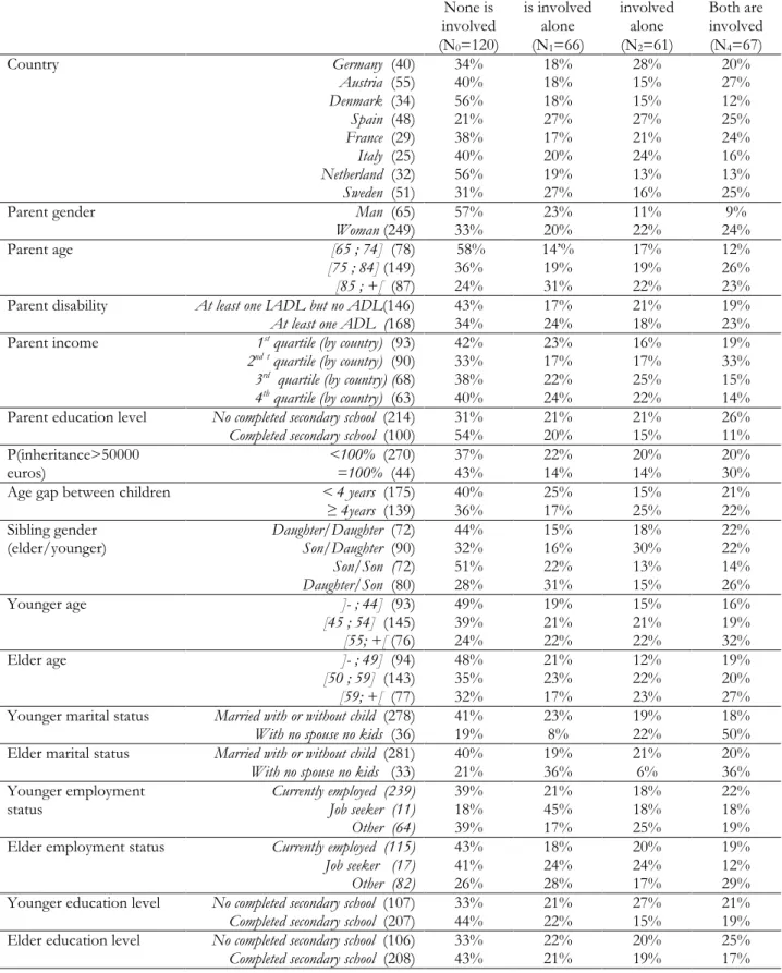
Table IV: Descriptive Statistics by care arrangements

Note: sub-sample size in parentheses.

Lecture: among the 40 elderly living in Germany, 35% does not receive any care from their children, 18% receive care from the elder, 28% receive care from the younger and 20% receive care from both of them.

None is involved The elder is involved alone The younger is involved alone Both are involved (N0=120) (N1=66) (N2=61) (N4=67) Country Germany (40) Austria (55) Denmark (34) Spain (48) France (29) Italy (25) Netherland (32) Sweden (51) 34% 40% 56% 21% 38% 40% 56% 31% 18% 18% 18% 27% 17% 20% 19% 27% 28% 15% 15% 27% 21% 24% 13% 16% 20% 27% 12% 25% 24% 16% 13% 25%

Parent gender Man (65)

Woman (249) 57% 33% 23% 20% 11% 22% 9% 24% Parent age [65 ; 74] (78) [75 ; 84] (149) [85 ; +[ (87) 58% 36% 24% 14’% 19% 31% 17% 19% 22% 12% 26% 23%

Parent disability At least one IADL but no ADL(146)

At least one ADL (168)

43% 34% 17% 24% 21% 18% 19% 23%

Parent income 1st _{quartile (by country) (93)}

2ndt _{quartile (by country) (90)}

3rd _{quartile (by country) (68)}

4th _{quartile (by country) (63)}

42% 33% 38% 40% 23% 17% 22% 24% 16% 17% 25% 22% 19% 33% 15% 14%

Parent education level No completed secondary school (214)

Completed secondary school (100)

31% 54% 21% 20% 21% 15% 26% 11% P(inheritance>50000 euros) <100% (270) =100% (44) 37% 43% 22% 14% 20% 14% 20% 30%

Age gap between children < 4 years (175)

≥ 4years (139) 40% 36% 25% 17% 15% 25% 21% 22% Sibling gender (elder/younger) Daughter/Daughter (72) Son/Daughter (90) Son/Son (72) Daughter/Son (80) 44% 32% 51% 28% 15% 16% 22% 31% 18% 30% 13% 15% 22% 22% 14% 26% Younger age ]- ; 44] (93) [45 ; 54] (145) [55; +[ (76) 49% 39% 24% 19% 21% 22% 15% 21% 22% 16% 19% 32% Elder age ]- ; 49] (94) [50 ; 59] (143) [59; +[ (77) 48% 35% 32% 21% 23% 17% 12% 22% 23% 19% 20% 27%

Younger marital status Married with or without child (278)

With no spouse no kids (36)

41% 19% 23% 8% 19% 22% 18% 50%

Elder marital status Married with or without child (281)

With no spouse no kids (33)

40% 21% 19% 36% 21% 6% 20% 36% Younger employment status Currently employed (239) Job seeker (11) Other (64) 39% 18% 39% 21% 45% 17% 18% 18% 25% 22% 18% 19%

Elder employment status Currently employed (115)

Job seeker (17) Other (82) 43% 41% 26% 18% 24% 28% 20% 24% 17% 19% 12% 29%

Younger education level No completed secondary school (107)

Completed secondary school (207)

33% 44% 21% 22% 27% 15% 21% 19%

Elder education level No completed secondary school (106)

Completed secondary school (208)

33% 43% 22% 21% 20% 19% 25% 17%

Appendix C

Table V: Selection rule effect

1

ˆ

β βˆ2

Endogeneous selection rule

{ }

ø ) 0.36; ˆ (1,

{ }

ø ) 0.22; ˆ (2,

{ }

ø) 0.22; (3,

{ }

ø) 0.21 , 0 ( ˆl = sel = sel = sêl = e s 1,089 (0,002) -0,718 (0,049)

Had hoc selection rule

(i)sel(0,

{ }

ø)=0.25;sel(1,

{ }

ø)=0.25;sel(2,

{ }

ø)=0.25;sel(3,

{ }

ø)=0.25 1,120 (0,003)

-0,789 (0,036)

(ii)sel(0,

{ }

ø)=1;sel(1,

{ }

ø)=0;sel(2,

{ }

ø)=0;sel(3,

{ }

ø)=0 0,729 (0,001)

-0,404 (0,162)

References

Andrews, D.W.K. 2001. Testing when a Parameter is on a Boundary of the Maintained

Hypothesis. Econometrica 69: 683-734.

Bjorn PA, Vuong QH. 1985. Simultaneous Equations Models for Dummy Endogenous

Variables: A Game Theoretic Formulation with application to Labor Force Participation. Working Paper n°537. Caltech. Pasadena. CA.

Bommier A. 1995. Peut-on compter sur ses enfants pour assurer ses vieux jours? L’exemple

de la Malaisie. Economie et Prévision 121 :75-86

Borsch-Supan A, Brugiavini A, Jürges H, Mackenbach J, Siegrist J, Weber G. 2005. Health, Ageing and Retirement in Europe: First Results from the Survey of Health, Ageing and Retirement in Europe, Mannheim: MEA.

Brock WA, Durlauf NA. 2001. Interactions-based models. in Handbook of Econometrics. Vol. 5. Heckman JJ, Laamer E (eds). North-Holland. Amsterdam. 3297-3380.

Byrne D, Goeree MS, Hiedemann B, Stern S. 2007. Formal Home Health Care, Informal Care, and Family Decision Making. Working paper

Checkovich T, Stern S. 2002. Shared Caregiving Responsibilities of Adult Siblings with

Elderly Parents. Journal of Human Resources 37(3): 441-478.

Engers M, Stern S. 2002. Long-Term Care and Family Bargaining. International Economic

Review 43(1): 73-114

Fontaine R, Gramain A, Wittwer J. 2007. Les configurations d'aide familiales mobilisées

autour des personnes âgées dépendantes en Europe. Economie et Statistique 403-404: 97-115.

Gouriéroux C, Holly A, Monfort A. 1982. Likelihood Ratio Tests, Wald Tests, and Kuhn-Tucker Test in Linear Models with Inequality Constraints on the Regression Parameters, Econometrica 50: 63-80.

Heckman J. 1978. Dummy endogenous variables in a simultaneous equation system.

Econometrica 46: 931-959.

Hiedemann B, Stern S. 1999. Strategic play among members when making long-term care

decisions. Journal of Economic Behavior & Organization 40(1): 29-57.

Jellal M, Wolff FC. 2002. Aides aux parents âgés et allocation intra-familiale. Revue

Économique 53(4): 863-885.

Konrad KA, Robledo JR. 2002. Geography of the family. American Economic Review 92(4):