S
EGMENTATION IN THE CRUDE OIL FUTURES TERM STRUCTURE
Delphine LAUTIER (*)
July 2004
Professional titles and affiliations: Professor, Ceros, University Paris X
Associate Research Fellow, Cerna, ENSMP
Mailing Address: Delphine Lautier
Ceros, Université Paris X
UFR Segmi, Bâtiment G,
200 avenue de la République
92 001 Cedex Nanterre
Telephone number: 33 1 43 26 98 89
Fax number: 33 1 40 97 71 42
Email: lautier @ cerna.ensmp.fr
(*) The author is very grateful for the helpful comments and suggestions of Professor Franklin Edwards (Columbia University).
S
EGMENTATION IN THE CRUDE OIL FUTURES TERM STRUCTURE
ABSTRACT: Whereas the spatial integration has already been examined in commodity markets, empirical tests on temporal integration have never been carried out. Relying on the “preferred habitat” theory, which is applied to the crude oil market, this article investigates whether this market is segmented or not. Segmentation is defined as a situation in which different parts of the prices curve are disconnected from each other. Consequently, the information conveyed by certain prices is useless when reconstituting the rest of the curve. Empirical tests are carried out with a term structure model, the performances of which depend on the informational value of the prices retained for the estimation. We show that the crude oil futures market is segmented into three parts. The first corresponds to maturities below 28 months, the second is situated between the 29th and 47th months, and the third consists of maturities ranging from the 4th to 7th years.
KEY WORDS:Information – futures prices – term structure – segmentation – crude oil.
INTRODUCTION
The term structure of commodity futures prices is the relationship linking the spot price and futures prices for different delivery dates. It synthesizes the information available in the market and the operators’ expectations concerning the future. This information is very useful for management purposes: it can be used to hedge exposures on the physical market or to adjust the stock level or production rate. It can also be used to undertake arbitrage transactions, to evaluate derivatives instruments based on futures contracts, etc.
There have been futures contracts for maturities extending up to seven years in the American crude oil market since 1999, rendering this information particularly abundant. Thus, this market provides publicly available prices – namely potentially informative and costless signals – whereas in most commodities markets, the only information for far maturities is private and given by forward prices. The introduction of these long-term futures contracts authorizes empirical studies on the crude oil prices’ curves that were only previously possible with forward prices. Yet the informational
content of the latter is not necessarily reliable or workable (the forward contracts are not standardized, the prices reporting mechanism does not force the operators to disclose their transactions prices, etc.).
This article aims to take advantage of the newly available information provided by the long-term crude oil futures contracts in order to improve the understanding of the futures prices’ behavior of storable commodities and also to facilitate the use of the term structure as a management tool. More precisely, its objective is to compare the informational content of futures prices for different maturities. It asks the following questions: do certain maturities provide more information than others? How much information does one specific futures price give about the rest of the prices curve? Is that information sufficient to reconstitute the whole term structure of futures prices? Are certain maturities more important for certain parts of the curve and irrelevant for the rest?
The answers given to these questions have crucial implications for financial decisions, particularly for all the hedging and valuation operations relying on the relationship between different futures prices. It is the case, for example, of the “stack and roll” hedging strategies that rely on short term futures contracts to protect long-term positions on the physical market (in 1994, Metallgesellschaft tried to build such a strategy in order to exploit the higher liquidity of the nearest contracts). The efficiency of these strategies can be affected by differences in the informational content of futures prices. It is also the case of investment decision, when the latter is based on the extrapolation from observed prices curves to value cash flows for maturities that are not available on the market1. All these operations rely on term structure models of commodity prices. Such a tool aims
to reproduce the futures prices observed in the market as accurately as possible and to extend the curve for very long maturities. However, its use requires the estimation of its parameters, and the latter may depend on the informational content of futures prices.
In this empirical study, it is supposed that, all things being equal, the performances of a term structure model (i.e. its ability to replicate the prices curve) depend on the informational value of the futures prices retained for its parameters’ estimation. The two-factor model proposed by Schwartz in 1997 – for which performances were firmly established on different commodity markets and different periods – authorizes the study of the futures prices’ informational content.
Two important conclusions are reached. First, each extremity of the prices curve has a specific and useful informational content. The differences between the two extremities are so high that the information concentrated on the nearest delivery dates is totally useless when reconstituting the long-term futures prices. This first result infers that the crude oil futures prices’ curve is segmented. Second, the study shows that from an informational point of view, there are three coherent groups of futures prices: the first corresponds to maturities ranging from the 1st to the 28th months, the second is situated between the 29th and 47th months, and the last consists of maturities between the 4th to 7th years. Among these groups, only two have real informational value: the first and the third. Thus, the prices curve is segmented into three parts.
Chances are high that this segmentation would evolve trough time, because since the date it was launched, the crude oil futures market has matured. Indeed, the New York Mercantile Exchange (Nymex) has experienced a growth in its transactions volume, pushing away the boundary of actively traded contracts. This phenomenon is reported in most derivatives markets, and one can expect that segmentation will move to longer maturities in the future. However, what is specific to the crude oil market is the introduction, since 1999, of long-term futures contracts. This created a new segment in the prices curve, which is separated from the shorter segment by intermediate maturities with no informational content. This long-term extremity of the curve is poorly connected with the nearest maturities. Thus, despite significant steps toward temporal integration, it is far from achieved in the case of the crude oil futures market.
The reasons explaining such a segmentation of the crude oil futures markets most likely be found in the “preferred habitat” theory, which supposes that different categories of participants are located at the two extremities of the curve: the hedgers, acting on the short term maturities, and the investors situated on far distant prices. Insufficient liquidity presumably prevents these operators from leaving their preferred habitat and undertaking arbitrage operations between maturities. The difficulty to initiate reverse cash and carry operations, due to the lack of physical stocks in markets characterized by backwardation, is another crucial explanatory factor in regards to the crude oil market. Moreover, there are ownership restrictions on the Nymex, that may prevent temporal integration. For example,
the rulebook of the exchange states that the position on crude oil futures contracts shall not exceed 20,000 contracts.
The article proceeds as follows. First, a brief analysis of the term structure of commodity futures prices is presented, and the central assumption of the paper is exposed. Second, the methodology of the empirical study, namely the term structure model retained, the method used to evaluate the informational content of futures prices, and the data, is exposed. Third, the empirical results are presented. The last section concludes.
1
For this kind of analysis, see for example Brennan and Schwartz (1985), Schwartz (1997, 1998), Cortazar and Schwartz (1998), Schwartz and Smith (2000), Cortazar et al (2001).
I.ANALYSIS OF THE TERM STRUCTURE OF COMMODITY FUTURES PRICES
The normal backwardation and storage theories are traditionally used to explain the relationship between spot and futures prices in commodity markets. Keynes introduced the normal backwardation theory in 1930. In his explanation, the difference between spot and futures prices is due to an unbalance between short and long hedging positions in the futures market. To compensate for this lack of balance, there is a need for speculators. A premium remunerates them for the risk they undertake in their activity. However, until now, the theory of normal backwardation was never truly validated nor rejected, most likely because the level and the direction of the risk premium are not constant.
The storage theory relies mainly on the storage costs and convenience yield to understand the situations of contango and backwardation. The concept of convenience yield was proposed by Kaldor in 1939. It can be briefly defined as the implicit gain associated with the holding of inventories. The stocks’ availability indeed prevents from production disruptions, and it makes it possible to take advantage of unexpected rises in demand (Brennan, 1958). The storage theory was validated on numerous commodity markets. It is the main theoretical basis for the elaboration of term structure models. However, when the analysis is centered on long-term horizon, one may ask if the explanatory factors of the storage theory are still of use.
Schwartz and Smith (2000), and Cortazar and Schwartz (2003) respond no to that question. They propose a theoretical analysis of the term structure of crude oil prices, in which different explanatory factors are distinguished, in step with the maturity of futures prices. Production, consumption, stocks’ level and the fear of inventories disruptions are the most important factors of the short term futures prices. For longer maturities, the explanatory factors change: interest rates, anticipated inflation and the prices for competing energies determine the futures prices.
If different market forces determine the short- and long-term futures prices, one may ask whether there is a temporal segmentation of the term structure. According to the market segmentation or preferred habitat approach to the term structure of interest rates (Modigliani and Sutch, 1966), segmentation can arise when a market participant has preferences for the holding of certain subsets of maturities, which might be termed the “preferred habitat” of that agent. In that situation, there exists a
separate supply and demand for assets at each habitat, which traders are reluctant to quit, unless they earn a sufficiently high return.
Many reasons were invoked to account for segmentation, which can be the result of institutional barriers such as taxes or restrictions on short sales. It is also explained by ownership restrictions, constraints on capital, information costs, management risks, etc. In the case of crude oil markets, the existence of preferred habitat could be due to the presence of several categories of participants in the futures market, each of them acting on different parts of the prices curve. Producers and consumers operate indeed primarily at the shorter end of the curve, whereas other investors, for example, banks, are located at the longer maturities.
Whereas the spatial integration has already been examined in the case of commodity markets – see for example Kleit (2001) or Milonas and Henker (2001) – empirical tests on temporal integration have never been carried out. This paper is an attempt to complement the existing literature on term structures of commodity prices by investigating this temporal integration. Segmentation is defined as a situation where different parts of the prices curve are disconnected from each other. As a result of segmentation, the crude oil futures prices curve should be separated into several parts, and the information conveyed by the prices should be of different nature when the contract’s maturity changes. The validation of this assumption should be valuable for the comprehension of prices behavior and for the use of term structure models as management tools.
II.METHODOLOGY
This section reveals the method used to evaluate the informational content of futures prices. This method relies on the use of a term structure model. It is supposed that the model’s performances depend on the informational value of the futures prices retained for the parameters’ estimation. The term structure model retained for the tests is first presented. Then, the data and the information sets chosen for the parameters estimation are exposed.
A. The term structure model
The first term structure model of commodity prices was proposed by Brennan and Schwartz in 1985. In this model, the behavior of the futures price is explained by one single variable: the spot price, which is assumed to follow geometric Brownian motion. This model, due to its simplicity, is not suited for long-term maturities. Indeed, the spot price dynamics ignores the fact that the operators in the physical market adjust their stocks to the evolution of the spot price and to the modifications of supply and demand. Moreover, this representation does not take into account the fact that a futures price depends not only on the spot price but also on the convenience yield. In this model, the convenience yield is a constant parameter. However, in 1989, Gibson and Schwartz showed that such an analysis is limited. They proposed to introduce the convenience yield as a second state variable. Schwartz (1997) has retained that proposition.
This author compares three term structure models of commodity prices. The first relies on a single state variable, and it is unable to correctly price the term structure of futures prices. The second is the two-factor model retained in this study. Because he thought that for long-term analysis, the interest rate should no longer be considered as a constant, Schwartz also introduced a stochastic interest rate in the third model. However, using forward prices provided by Enron, he showed that the two- and three-factor models are very similar empirically. Thus, the three-factor model is of little interest. In addition, the two-factor model has proven its ability to reproduce the term structure of futures prices on the crude oil and cooper markets, on the shorter as well as longest maturities, and throughout several periods. Moreover, it is of relatively easy use because it is linear and has an
analytical solution. Finally, it was used as a reference to develop more sophisticated models2. All these
reasons lead retaining it for the empirical study conducted in this article.
The two-factor model supposes that the spot price S and the convenience yield C can explain the behavior of the futures price F. The dynamic of these state variables is:
(
)
[
]
⎩
⎨
⎧
+
−
=
+
−
=
C C S Sdz
dt
C
k
dC
Sdz
Sdt
C
dS
σ
α
σ
µ
)
(
(1) with: κ, σS, σC >0where: - µ is the drift of the spot price,
-
σ
S is the spot price volatility,- dzS is an increment to a standard Brownian motion associated with S,
- α is the long run mean of the convenience yield, - κ is the speed of adjustment of the convenience yield, -
σ
C is the volatility of the convenience yield,- dzC is an increment to a standard Brownian motion associated with C.
In this model, the convenience yield is mean-reverting. This formulation relies on the hypothesis that there is a level of stocks which satisfies the needs of industry under normal conditions. The behavior of the operators in the physical market guarantees the existence of this normal level. When the convenience yield is low, the stocks are abundant and the operators sustain a high storage cost compared with the benefits related to holding the raw materials. So if they are rational, they try to reduce these surplus stocks. Conversely, when the stocks are rare the operators tend to reconstitute them.
Moreover, as the storage theory shows it, the two state variables are correlated. Both the spot price and the convenience yield are an inverse function of the inventories level. Nevertheless, as Gibson and Schwartz (1990) demonstrate, the correlation between these two variables is not perfect. Therefore, the increments to standard Brownian motions are correlated, with:
[
dz
dz
]
dt
E
S×
C=
ρ
An arbitrage reasoning and the construction of a hedge portfolio lead to the solution of the model. It expresses the relationship at t between an observable futures price F for delivery at T and the state variables S and C. This solution is:
( )
⎥ ⎦ ⎤ ⎢ ⎣ ⎡ + − − × = − τ κ κτ B e t C t S T t C S F( , , , ) ( ) exp ( )1 (2) with: -( )
⎥
⎦
⎤
⎢
⎣
⎡
⎟⎟
⎠
⎞
⎜⎜
⎝
⎛ −
×
⎟⎟
⎠
⎞
⎜⎜
⎝
⎛
−
+
+
⎥
⎦
⎤
⎢
⎣
⎡
−
×
+
⎥
⎦
⎤
⎢
⎣
⎡
×
⎟⎟
⎠
⎞
⎜⎜
⎝
⎛
−
+
−
=
22 21
3−2 21
2−4
2
κ
κ
σ
ρ
σ
σ
κ
α
κ
σ
τ
κ
ρ
σ
σ
κ
σ
α
τ
r
e
κτe
κτB
C C S C C S C)
)
- α)=α−(
λ /κ)
where: - r is the risk free interest rate, assumed constant, - λ is the market price of convenience yield risk, - τ = T - t is the maturity of the futures contract.
The model’s performances measure its ability to reproduce the term structure of commodity prices. To assess these performances, parameters values and criteria are needed. The parameters values are necessary to compute the estimated futures prices and to compare them with empirical data. The parameters estimation is not obvious though, because like many term structure models, that of Schwartz relies on non-observable state variables. Both the spot price and the convenience yield are indeed regarded as non-observable because most of the time there are no reliable time series for the spot price and the convenience yield is not a traded asset. In order to deal with this difficulty, the method proposed by Schwartz in 1997, a Kalman filter, is used3.
B. Performance criteria
The model’s performances measure its ability to reproduce the term structure of commodity prices. To assess these performances, two criteria were retained: the mean pricing error and the root mean squared error.
The mean pricing error (MPE) is defined as follows:
( ) ( )
(
)
∑
= − = N n n F n F N MPE 1 , , ~ 1 τ τ (3)where N is the number of observations, F~
( )
n,τ is the estimated futures price for a maturity τ at date n and F( )
n,τ is the observed futures price. The MPE is expressed in US dollar. It measures the estimation bias for one given maturity. When the estimation is good, the MPE is close to zero.Retaining the same notations, the root mean squared error (RMSE) is also expressed in US dollar and is defined in the following way, for one given maturity τ :
( ) ( )
(
)
∑
= − = N n n F n F N RMSE 1 2 , , ~ 1 τ τ (4)When there is no bias, the RMSE can be considered as an empirical variance. It measures the estimations stability. This second criterion is considered as more representative because prices errors can offset themselves and the MPE can be low even if there are strong deviations.
Relying on these criteria, the sensitivity of the model performances to the information used for the estimation can be tested. This information is constituted of temporal series of futures prices corresponding to a few selected maturities.
C. Information used
In this study, the informational content of futures prices is assumed to be captured by the parameters of the model. In order to measure this informational content, several sets of futures prices having various maturities are selected and used for the estimation of the parameters. Each set gathers four maturities4, which are then used to determine, at each observation date, the corresponding futures
prices (first for the four maturities selected, afterwards for those remaining). These prices constitute a theoretical curve based upon a specific information set. Lastly, relying on the performance criteria previously defined, this curve is compared with the empirical one observed at the same date. Such a comparison throughout the whole study period makes it possible to appreciate whether the maturities set retained contains enough information to correctly reconstitute the curve. The repetition of this test with different sets of maturities makes it possible to investigate whether certain sets lead to better performances, that is whether they provide more information, than do others.
The empirical tests are carried out with seven sets of maturities. In order to examine the value of the assumption, according to which the short- and the long-term futures prices are influenced by different factors, the two extremities of the prices curve are first retained: the nearby delivery months (1st, 2nd, 3rd and 4th), and the longer maturities (48th, 60th, 72nd, and 84th months). Then, while retaining the information on the shorter expiration date (1st month), the other maturities are progressively moved away. Thus, the parameters corresponding to the 1st, 3rd, 6th, and 9th months are estimated. Then the 1st, 5th, 10th, and 15th months are used. The fifth set corresponds to the 1st, 6th, 12th, and 18th months, and the sixth to the 1st, 12th, 24th and 48th months. Finally, a set with maturities regularly distributed along the prices curve, which gathers the 1st, 24th, 48th, and 84th months, is retained.
D. Data
The database is an important element of the study. Considering the volume and the maturity of the transactions, the American crude oil futures market is today the most developed commodity futures market. Thus, working with crude oil prices makes it possible to study maturities up to seven years in advance5. The database covers the period from 06/01/1999 to 01/14/02. The crude oil prices are daily settlement prices for the West Texas Intermediate futures contract of the New York Mercantile Exchange. They have been operated in the following manner: the first futures price maturity corresponds to the one month maturity, the second futures price corresponds to the two months maturity, and so forth. Lastly, weekly data were retained for the estimations (139 weeks).
The choice of the temporal series of futures prices is guided by liquidity concerns. On the crude oil market, as on other commodity markets, the transaction volume is always higher on the nearest maturities. However, the crude oil market is also characterized by a lack of liquidity on intermediate maturities: there are no regularly available data, on the study period, for the futures contracts corresponding to maturities situated between the 29th and 47th months. Thus, they are removed from the database. Finally, thirty-two different maturities are selected. From the 1st to 28th month, each temporal series corresponds to the maturity of a futures contract. On a longer horizon, the maturities for the 48th, 60th, 72nd, and 84th delivery months are also retained.
The interest rates are daily T-bill rates for a three months maturity and are extracted from Datastream. Because interest rates are presumed constant in the model, the mean of the observations between June 1999 and January 2002 is retained.
2
In 1998, Hilliard and Reis proposed to introduce jumps in the spot price process in order to take into account the large and abrupt changes due to supply and demand shocks, which affect certain commodity markets (especially energy commodities used for heating). Schwartz and Smith (2000) proposed a short term/long term model, which is equivalent to the Schwartz (1997) two-factor model, in that the state variables in one of the models can be expressed as linear combinations of the state variables in the other model. Lautier and Galli (2001) introduced a mean-reverting convenience yield with asymmetrical behavior. This representation
expresses the fact that in commodity markets, the basis is more volatile in backwardation than in contango. Yan (2002) introduced a stochastic volatility.
3
Appendix 1 presents this method.
4
This number of maturities is retained because it increases the stability of the estimation procedure.
5
However, the transaction volume is not very high for the longer maturities. Therefore, the quality of the information conveyed by those prices may not be excellent.
III.EMPIRICAL RESULTS
This section presents the empirical results. The model’s performances as well as their sensitivity to the informational content of the parameters are analyzed. Then the parameters obtained with the seven maturities’ sets are exposed.
A. The model’s performances and their sensitivity to the information used
The model’s performances are first of all presented for all the maturities retained in the study. However, the nature of the results leads to separating the shorter and longer maturities.
Reconstitution of the prices curve
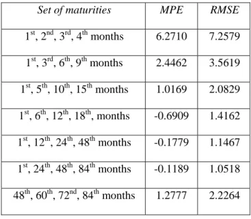
Table I illustrates the MPE and RMSE obtained on the study period, for all the maturities. Each line represents the averages MPE and RMSE related to a specific information set (i.e. one set of parameters). Appendix 2 provides all of the results, one maturity at a time.
The empirical tests carried out on the study period imply two statements. First, the informational content of futures prices changes with the contract’s expiration date. Indeed, the choice of a specific maturities’ set significantly alters the model’s performances. Its ability to reproduce the prices curve is weak with the shorter maturities, and very acute with the set gathering the 1st, 24th, 48th, and 84th months. Thus, even if Schwartz’ model supposes that the interest rate is constant and ignores political risk or eventual shocks on demand and supply, it is suited for the replication of the shorter as well as the longer part of the prices curve (MPE lower than 12 cents, and average RMSE around USD 1.05), provided the proper information set is retained. Second, each extremity of the prices curve has a useful and specific informational content. Indeed, the best performances are achieved with the set including the two extremities. Thus, both extremities provide useful information for the reconstitution of the prices curve, and their informational content is different, as the observation of the performances associated with each extremity (lines 2 and 8 of Table I) corroborates. This leads to examining the shorter and longer maturities separately.
The shorter part of the curve
Table II exposes the average MPE and RMSE obtained with a shortened prices curve: from the 1st to 28th months.
The elimination of the end of the curve makes it possible to infer a third statement: the observation of the MPE and the RMSE month per month (see Appendix 2) shows that there are no sizeable differences between the performances obtained with the maturities ranging from the 1st to the 28th months. Focusing on the shorter part of the curve brings together the performances of the different maturity sets and shows that the shorter maturities can be reasonably retained in order to reconstitute the curve up to 28 months. Moreover, the performances of the first set of parameters are dramatically improved: when compared with Table II, the RMSE falls from USD 7.2579 to USD 1.7463.
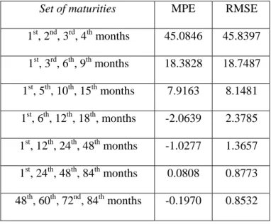
The longer part of the curve
The focus on the longer part of the curve (4th to 7th years), illustrated by Table III, brings forth a fourth statement: the information concentrated on the shorter maturities is useless reconstituting the end of the prices curve. Indeed, when estimated on the nearest maturities, Schwartz’ model leads to long-term futures prices with no economical sense: the averages MPE are around USD 45 per barrel!
B. Parameters
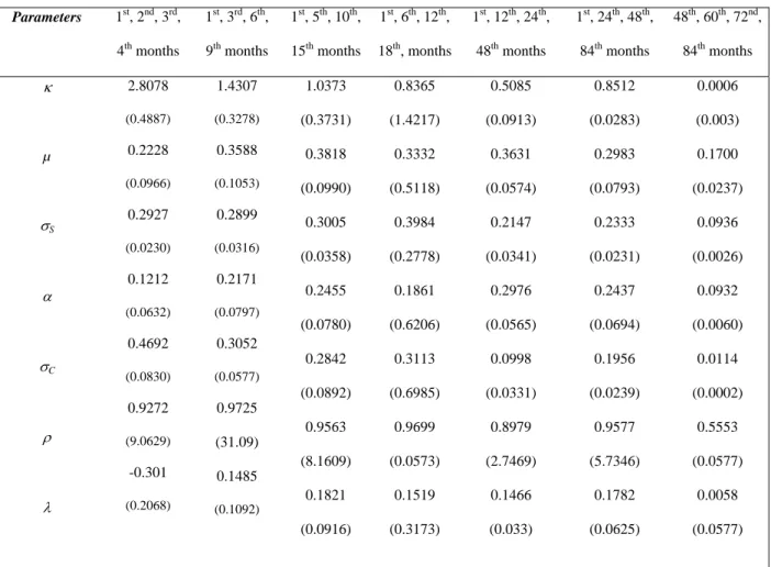
The last empirical results presented are the optimal parameters corresponding to each set of maturities. Schwartz’ model includes seven parameters, all of them presumed constant. Nevertheless, in 1997, relying on forward prices for long-term expiration dates, the author showed that they change with the maturities retained for the estimation. Table IV illustrates that the same result is reached with futures prices.
The most important changes concern the speed of adjustment of the convenience yield, the volatilities of the two state variables and their correlation coefficient. All of them tend to decrease with maturity. Indeed, in the model mean reversion concerns the stocks, which are of little importance for long-term maturities. As a result, a low speed of adjustment characterises the longer part of the curve. The same kind of explanation can be evoked for the volatilities. Their level decreases when the
maturity rises because the shocks on supply and demand have then a lowest impact on the futures prices. Considering these changes, the parameters of the term structure models should ideally be maturity dependent: the speed of adjustment and the volatilities of the state variables should be considered as decreasing functions of the expiration date. However, since the parameters are also time-dependent, such a modification will strongly improve the model’s complexity.
IV.CONCLUSION AND POLICY IMPLICATIONS
This article is centered on the informational value of futures prices. The significance of the study lies in a better understanding of the behavior of the term structure of commodity prices and an enhanced appreciation of the way to use the term structure models for management purposes. Relying on the performances of Schwartz’ model to appreciate the informational content of futures prices, this empirical study shows that the information conveyed by the prices changes with the contract’s maturity. More precisely, two important conclusions can be drawn.
First, each extremity of the prices curve has a specific and useful informational content. Second, from an informational point of view, there are three coherent groups of futures prices: the first corresponds to maturities ranging from the 1st to 28th month, the second is situated between the 29th and 47th months, and the last consists of maturities from the 4th to 7th year. Among these groups, only two have a real informational value: the first and the third. Thus, the prices curve is segmented into three parts.
The segmentation of the crude oil market has key policy implications. Indeed, term structure models are used for hedging and investment purposes. However, as this article shows, one must be very cautious when using such a model to extend the prices curve. The model must not only be well-suited for long-term applications. The information used for the estimation is also crucial because it significantly alters the model’s performances. When the proper set of maturities is chosen – namely, the two extremities of the curve – the ability of Schwartz’ model to reproduce the futures prices for very long maturities is excellent. However, the same model can lead to prices with no economical sense if the nearest futures prices are used to reconstitute those of the long-term.
Further work could be undertaken. Another investigation relying on the private information given by forward prices for maturities extending more than seven years could lead to the discovery of new segments in the crude oil market. The same methodology could also be reproduced on other periods, in order to examine if the segmentation really with time. Such studies would lead to a more accurate use of the information and the hedging instruments provided by the futures markets.
BIBLIOGRAPHY
Brennan, M.J. (1958). “The supply of storage.” American Economic Review, 47(1): 50-72.
Brennan, M.J., & Schwartz, E.S.(1985). “Evaluating natural resource investments.” The Journal of Business, 58(2): 135-157.
Cortazar, G., & Schwartz, E.S. (1998). “Monte-carlo evaluation model of an undeveloped oil field.” Journal of Energy Finance and Development, 3(1): 73-84.
Cortazar, G., Schwartz, E.S., & Casassus, J. (2001). “Optimal exploration investments under price and geological-technical uncertainty: a real options model.” R & D Management, 31: 181-189.
Cortazar, G., & Schwartz, E.S. (2003). ”Implementing a Stochastic Model for Oil Futures Prices.” Energy Economics, 25: 215-238.
Gibson, R., & Schwartz, E.S. (1989). “Valuation of long-term oil-linked assets.” Working Paper, Anderson Graduate School of Management, UCLA.
Gibson, R., & Schwartz, E.S.(1990).“Stochastic convenience yield and the pricing of oil contingent claims.” Journal of Finance, 45(3): 959-975.
Harvey, A.C. (1989). Forecasting, structural time series models and the Kalman filter, Cambridge, England: Cambridge University Press.
Hilliard, J.E., & Reis, J. (1998). “Valuation of commodity futures and options under stochastic convenience yield, interest rates, and jump diffusions in the spot.” Journal of Financial and Quantitative Analysis, 33(1): 61-86.
Kaldor, N. (1939). “A note on the theory of the forward market.” Review of Economic Studies, 8(1): 196-201.
Keynes, J.M. (1930). A Treatise on Money: The applied Theory of Money. Londres, England: Macmillan, vol. 2.
Kleit, A.N. (2001). “Are regional oil markets growing closer together? An arbitrage cost approach”. Energy Journal, 22 : 1-15.
Lautier, D., & Galli, A. (2001). “A term structure model of commodity prices with asymmetrical behaviour of the convenience yield”, Fineco, 11: 73-95.
oil market.” Applied financial economics, 11: 23-36.
Modigliani, F., & Sutch, R. (1966). “Innovations in interest rate policy.” American Economic Review, 56: 178-197.
Schwartz, E.S.(1997).“The stochastic behavior of commodity prices: implications for valuation and hedging.” The Journal of Finance, 52(3): 923-973.
Schwartz, E.S. (1998). “Valuing long-term commodity assets.” Journal of Energy Finance and Development, 3(2): 85-99.
Schwartz, E.S., & Smith, J.E. (2000). “Short-term variations and long-term dynamics in commodity prices”. Management Science, 46: 893-911.
Yan X., (2002). “Valuation of commodity derivatives in a new multi-factor model”. Review of Derivatives Research, 5: 251-271.
Table I. Average MPE and RMSE for all the maturities
Set of maturities MPE RMSE
1st, 2nd, 3rd, 4th months 6.2710 7.2579 1st, 3rd, 6th, 9th months 2.4462 3.5619 1st, 5th, 10th, 15th months 1.0169 2.0829 1st, 6th, 12th, 18th, months -0.6909 1.4162 1st, 12th, 24th, 48th months -0.1779 1.1467 1st, 24th, 48th, 84th months -0.1189 1.0518 48th, 60th, 72nd, 84th months 1.2777 2.2264 Unit : USD/b
Table II. Average MPE and RMSE for the 1st to 28th months
Set of maturities MPE RMSE
1st, 2nd, 3rd, 4th months 0.7262 1.7463 1st, 3rd, 6th, 9th months 0.1696 1.3924 1st, 5th, 10th, 15th months 0.0312 1.2165 1st, 6th, 12th, 18th, months -0.4948 1.2787 1st, 12th, 24th, 48th months -0.0565 1.1154 1st, 24th, 48th, 84th months -0.1474 1.0767 48th, 60th, 72nd, 84th months 1.4884 2.4225 Unit : USD/b
Table III. Average MPE and RMSE for the 4th to 7th years
Set of maturities MPE RMSE
1st, 2nd, 3rd, 4th months 45.0846 45.8397 1st, 3rd, 6th, 9th months 18.3828 18.7487 1st, 5th, 10th, 15th months 7.9163 8.1481 1st, 6th, 12th, 18th, months -2.0639 2.3785 1st, 12th, 24th, 48th months -1.0277 1.3657 1st, 24th, 48th, 84th months 0.0808 0.8773 48th, 60th, 72nd, 84th months -0.1970 0.8532 Unit : USD/b
Table IV. Optimal parameters corresponding to each set of maturities Parameters 1st, 2nd, 3rd, 4th months 1st, 3rd, 6th, 9th months 1st, 5th, 10th, 15th months 1st, 6th, 12th, 18th, months 1st, 12th, 24th, 48th months 1st, 24th, 48th, 84th months 48th, 60th, 72nd, 84th months κ µ σS α σC ρ λ 2.8078 (0.4887) 0.2228 (0.0966) 0.2927 (0.0230) 0.1212 (0.0632) 0.4692 (0.0830) 0.9272 (9.0629) -0.301 (0.2068) 1.4307 (0.3278) 0.3588 (0.1053) 0.2899 (0.0316) 0.2171 (0.0797) 0.3052 (0.0577) 0.9725 (31.09) 0.1485 (0.1092) 1.0373 (0.3731) 0.3818 (0.0990) 0.3005 (0.0358) 0.2455 (0.0780) 0.2842 (0.0892) 0.9563 (8.1609) 0.1821 (0.0916) 0.8365 (1.4217) 0.3332 (0.5118) 0.3984 (0.2778) 0.1861 (0.6206) 0.3113 (0.6985) 0.9699 (0.0573) 0.1519 (0.3173) 0.5085 (0.0913) 0.3631 (0.0574) 0.2147 (0.0341) 0.2976 (0.0565) 0.0998 (0.0331) 0.8979 (2.7469) 0.1466 (0.033) 0.8512 (0.0283) 0.2983 (0.0793) 0.2333 (0.0231) 0.2437 (0.0694) 0.1956 (0.0239) 0.9577 (5.7346) 0.1782 (0.0625) 0.0006 (0.003) 0.1700 (0.0237) 0.0936 (0.0026) 0.0932 (0.0060) 0.0114 (0.0002) 0.5553 (0.0577) 0.0058 (0.0577)
The parameters values retained to initiate the optimization are: κ = 0.5 ; µ = 0.1 ; σS = 0.3 ; α = 0.1 ; σC = 0.4 ; ρ = 0.5 ; λ =
0.1. Standard deviations are in parentheses. For two sets of maturities (the 4th and 7th) the parameters are obtained with a
APPENDIX 1.KALMAN FILTER AND PARAMETERS’ ESTIMATION
The Kalman filters are powerful tools, which can be used for models estimation in many areas in finance. A Kalman filter is an interesting method when a large volume of information must be taken into account, because it is very fast. When associated with an optimization procedure, it can also be used for the estimation of the parameters, if the model relies on non-observable data.
The simple Kalman filter is the most common version of the Kalman filter. It can be used when the model is linear, as is the case for Schwartz’ model. First, the main principles of the method are presented. Second, the parameters estimation is exposed.
1. Presentation6
The main principle of the Kalman filter is to use temporal series of observable variables in order to reconstitute the value of non-observable variables. The model has to be expressed in a state-space form characterized by a transition equation and a measurement equation. Once this has been made, a three step iteration process can begin.
The state-space form model, in the simple filter, is characterized by the following equations:
• Transition equation: t t t t Tα c Rη α / −1= −1+ + (5)
where αt is the m-dimensional vector of non-observable variables at t, also called state vector, T is a
matrix (m × m), c is an m-dimensional vector, and R is (m × m) • Measurement equation: t t t t t Z d y / −1= α / −1+ +ε (6)
where yt/t−1 is an N-dimensional temporal series, Z is a (N×m) matrix, and d is an N-dimensional
vector.
t
η
andε
tare white noises, which dimensions are respectively m and N. They are supposed to be normally distributed, with zero mean and with Q and H as covariance matrices:[ ]
t=
0
E
η
andVar
[ ]
η
t=
Q
[ ]
t=
0
E
ε
andVar
[ ]
ε
t=
H
The initial value of the system is supposed to be normal, with mean and variance:
[ ]
α0 =α~0E ,
Var
[ ]
α
0=
P
0If α~ is a non biased estimator of αt t, conditionally to the information available in t, then:
[
t −~ =t]
0t
E α α
Consequently, the following expression7 defines the covariance matrix P
t :
(
)(
)
[
~t t ~t t ']
t t E P = α −α α −αDuring the iteration, three steps are successively tackled: prediction, innovation and updating.
• Prediction: ⎩ ⎨ ⎧ + = + = − − − − ' ' ~ ~ 1 1 / 1 1 / R Q R T P T P c T t t t t t t α α (7)
where α~t/t−1 and Pt / t-1 are the best estimators of αt/t-1 and Pt/t-1 , conditionally to the information
available at (t-1). • Innovation: ⎪ ⎩ ⎪ ⎨ ⎧ + = − = + = − − − − H Z ZP F y y v d Z y t t t t t t t t t t t ' ~ ~ ~ 1 / 1 / 1 / 1 / α (8)
where ~yt/t−1 is the estimator of the observation yt conditionally to the information available at (t-1),
and vt is the innovation process, with Ft as a covariance matrix.
• Updating: ⎪⎩ ⎪ ⎨ ⎧ − = + = − − − − − − 1 / 1 1 / 1 1 / 1 / ) ' ( ' ~ ~ t t t t t t t t t t t t t P Z F Z P I P v F Z P α α (9)
The matrices T, c, R, Z, d, Q, and H are the system matrices associated with the state-space
2. Parameters’ estimation
When the Kalman filter is applied to term structure models of commodity prices, the aim is the estimation of the parameters of the measurement equation, in order to obtain estimated futures
prices for different maturitiesF~
( )
τi , and to compare them with empirical futures pricesF( )
τi . The closest the firsts are with the seconds, the best is the model.Suppose that the non-observable variables and the errors are normally distributed. Then the Kalman filter can be used to estimate the model parameters, which are supposed to be constant. On that purpose, the logarithm of the likelihood function is computed for the innovation vt, for given
iteration and parameters vector:
t t t t
v
F
v
dF
n
t
l
⎟
×
Π
−
−
×
×
⎠
⎞
⎜
⎝
⎛
−
=
−1'
2
1
)
ln(
2
1
)
2
ln(
2
)
(
log
(10)where Ft is the covariance matrix associated with the innovation vt, and dFt its determinant8.
Relying on the hypothesis that the model measurement equation admits continuous partial derivatives of first and second order on the parameters, another recursive procedure is used to estimate the parameters9. An initial M-dimensional vector of parameters is first used to compute the
innovations and the logarithms of the likelihood function. Then the iterative procedure researches the parameters vector that maximizes the likelihood function and minimizes the innovations. Once this optimal vector is obtained, the Kalman filter is used, for the last time, to reconstitute the
non-observable variables and the measure y~ associated with these parameters.
3. Application to Schwartz’ model
The simple Kalman filter can be applied to Schwartz’ model because the later can be easily expressed on a linear form, as follows:
(
)
( )
( )
τ κ κτ B e t C t S T t C S F = − × − + − 1 ) ( ) ( ln ) , , , ( ln (11)Letting G = ln(S), we also have:
(
)
[
]
⎪⎩ ⎪ ⎨ ⎧ + − = + − − = C C S S S dz dt C k dC dz dt C dG σ α σ σ µ ) 2 1 ( 2 (12)The transition equation is:
t t t t t t t R C G T c C G + η ⎥ ⎥ ⎦ ⎤ ⎢ ⎢ ⎣ ⎡ × + = ⎥ ⎥ ⎦ ⎤ ⎢ ⎢ ⎣ ⎡ − − − − 1 1 1 / 1 / ~ ~ ~ ~ , t = 1, ... NT (13) where: - ⎥ ⎥ ⎦ ⎤ ⎢ ⎢ ⎣ ⎡ ∆ ∆ ⎟ ⎠ ⎞ ⎜ ⎝ ⎛ − = t t c S
κα
σ
µ
2 2 1is a (2×1) vector, and ∆t is the period separating 2 observation dates
-
⎥
⎦
⎤
⎢
⎣
⎡
∆
−
∆
−
=
t
t
T
κ
1
0
1
is a (2 × 2) matrix,- R is the identity matrix, (2 × 2),
- ηt are uncorrelated errors, with :
E[ηt] = 0, and ⎥ ⎦ ⎤ ⎢ ⎣ ⎡ ∆ ∆ ∆ ∆ = = t t t t Var Q C C S C S S t 2 2 ] [
σ
σ
ρσ
σ
ρσ
σ
η
The measurement equation is:
t t t t t t t C G Z d y +ε ⎥ ⎥ ⎦ ⎤ ⎢ ⎢ ⎣ ⎡ × + = − − − 1 / 1 / 1 / ~ ~ ~ , t = 1, ... NT (14) where:
- the ith line of the N dimensional vector of the observable variables ~yt/t−1 is
[
ln( )
F~( )
τi]
, with i = 1,..,N, where N is the number of maturities retained for the estimation.- d = [B(τi)] is the i
th
line of the d vector, with i = 1,..., N
- ⎥ ⎦ ⎤ ⎢ ⎣ ⎡ − − = −
κ
κτi eZ 1 , 1 is the ith line of the Z matrix, which is (N×2), with i = 1,...,N
- εt is a white noise’s vector, (N×1), with no serial correlation : E[εt] = 0 and H = Var[εt]. H is
6
Harvey (1989) inspires this presentation.
7
(
)
' ~
t t α
α − is the transposed matrix of
(
α~t−αt)
.8
The value of logl(t) is corrected when dFt is equal to zero.
9
APPENDIX 2.THE MODEL PERFORMANCES FOR ALL THE MATURITIES
1-2-3-4 1-3-6-9 1-5-10-15 1-6-12-18 1-12-24-48 1-24-48-84 48-60-72-84
M aturity MPE RMSE MPE RMSE M PE RM SE MPE RMSE M PE RM SE MPE RMSE MPE RM SE
1 month -0,2160 2,2207 0,0961 2,1769 0,1048 1,9196 -0,5356 2,3705 0,2025 2,2266 0,1419 1,9311 0,0685 2,7829 2 months -0,1676 2,0503 -0,0102 1,9847 -0,0107 1,7862 -0,5391 2,1169 0,1124 1,9223 0,0156 1,6889 -0,0133 2,4780 3 months -0,1592 1,9154 -0,0951 1,8438 -0,1044 1,6646 -0,5336 1,9033 0,0378 1,6740 -0,0828 1,4987 -0,0982 2,2194 4 months -0,1519 1,7992 -0,1316 1,7314 -0,1484 1,5476 -0,4892 1,7083 0,0079 1,4767 -0,1260 1,3544 -0,1554 2,0079 5 months -0,0208 1,8062 -0,0216 1,7311 0,0332 1,5436 -0,6161 1,8228 -0,0428 1,5843 0,0007 1,4143 -0,3180 1,8908 6 months -0,0169 1,6871 -0,0046 1,6283 0,0309 1,4307 -0,5247 1,6195 -0,0305 1,4085 -0,0489 1,2776 -0,2795 1,7063 7 months -0,0504 1,5846 0,0077 1,5468 0,0284 1,3435 -0,4403 1,4476 -0,0201 1,2667 -0,0890 1,1776 -0,2573 1,5529 8 months -0,1169 1,4979 0,0130 1,4807 0,0233 1,2763 -0,3645 1,3033 -0,0136 1,1542 -0,1231 1,1077 -0,2522 1,4261 9 months 0,6591 1,7346 0,0165 1,4975 -0,0105 1,3295 -0,6537 1,5074 -0,1095 1,2766 -0,1328 1,1759 0,8705 1,6755 10 months 0,5391 1,6043 0,0236 1,4304 -0,0123 1,2612 -0,5641 1,3577 -0,0865 1,1646 -0,1469 1,1007 0,8404 1,5698 11 months 0,4026 1,4804 0,0262 1,3702 -0,0134 1,2030 -0,4783 1,2239 -0,0633 1,0695 -0,1540 1,0399 0,8011 1,4706 12 months 0,2538 1,3699 0,0255 1,3167 -0,0132 1,1540 -0,3948 1,1063 -0,0387 0,9911 -0,1539 0,9917 0,7545 1,3787 13 months 1,1760 1,8505 0,1517 1,3510 0,0134 1,2136 -0,6442 1,3158 -0,1583 1,1011 -0,2152 1,0709 1,8015 2,2333 14 months 0,9826 1,6709 0,1557 1,2917 0,0284 1,1533 -0,5417 1,1806 -0,1154 1,0134 -0,1948 1,0068 1,7248 2,1317 15 months 0,7799 1,5012 0,1503 1,2376 0,0382 1,1005 -0,4458 1,0608 -0,0759 0,9387 -0,1744 0,9515 1,6393 2,0283 16 months 0,5674 1,3494 0,1339 1,1909 0,0413 1,0571 -0,3578 0,9596 -0,0415 0,8790 -0,1559 0,9075 1,5439 1,9222 17 months 1,5711 2,0636 0,3785 1,3113 0,0937 1,1466 -0,5842 1,1599 -0,1367 0,9918 -0,2327 1,0041 2,5152 2,8823 18 months 1,3219 1,8426 0,3471 1,2593 0,0996 1,1025 -0,4889 1,0546 -0,0968 0,9289 -0,2004 0,9521 2,3927 2,7494 19 months 1,0648 1,6280 0,3040 1,2058 0,0960 1,0591 -0,4027 0,9607 -0,0636 0,8717 -0,1736 0,9041 2,2608 2,6081 20 months 0,8041 1,4296 0,2531 1,1535 0,0868 1,0177 -0,3218 0,8768 -0,0332 0,8205 -0,1488 0,8600 2,1234 2,4629 21 months 1,7668 2,1678 0,2969 1,2135 -0,0147 1,0483 -0,6652 1,1911 -0,1317 0,8949 -0,2747 0,9112 3,0253 3,3939 22 months 1,4796 1,9127 0,2298 1,1586 -0,0341 1,0091 -0,5886 1,1149 -0,1022 0,8439 -0,2390 0,8664 2,8695 3,2293 23 months 1,1748 1,6550 0,1405 1,0992 -0,0744 0,9687 -0,5325 1,0568 -0,0911 0,8000 -0,2224 0,8289 2,6937 3,0408 24 months 0,9027 1,4503 0,0793 1,0651 -0,0855 0,9433 -0,4468 0,9893 -0,0486 0,7632 -0,1753 0,7943 2,5481 2,8956 25 months 1,9020 2,2914 0,6767 1,2781 0,2087 0,9953 -0,5405 0,9562 -0,1603 0,8478 -0,2566 0,8861 3,3981 3,7883 26 months 1,5959 2,0222 0,5900 1,2086 0,1832 0,9608 -0,4633 0,8808 -0,1284 0,8082 -0,2229 0,8487 3,2278 3,6101 27 months 1,2941 1,7700 0,5025 1,1429 0,1571 0,9282 -0,3859 0,8110 -0,0945 0,7724 -0,1883 0,8142 3,0590 3,4347 28 months 0,9954 1,5397 0,4131 1,0811 0,1293 0,8971 -0,3095 0,7485 -0,0598 0,7404 -0,1539 0,7827 2,8906 3,2610 48 months 66,1569 67,0793 23,7877 24,1712 10,1052 10,3425 -2,6051 2,9408 -1,4159 1,7768 -0,0196 1,0849 -0,2572 0,8673 60 months 50,2521 51,0392 20,0129 20,3778 8,6222 8,8483 -2,2986 2,6083 -1,2274 1,5405 0,0971 0,9218 -0,2246 0,8291 72 months 37,2891 37,9790 16,5183 16,8774 7,2011 7,4291 -1,8768 2,1826 -0,8957 1,2133 0,1595 0,7993 -0,1659 0,8280 84 months 26,6402 27,2612 13,2121 13,5685 5,7366 5,9723 -1,4749 1,7824 -0,5717 0,9324 0,0862 0,7031 -0,1400 0,8883