Efficient gradient method for locally optimizing the periodic/aperiodic ambiguity function

HAL Id: hal-01325271

https://hal.archives-ouvertes.fr/hal-01325271

Submitted on 2 Jun 2016

HAL is a multi-disciplinary open access

archive for the deposit and dissemination of

sci-entific research documents, whether they are

pub-lished or not. The documents may come from

teaching and research institutions in France or

abroad, or from public or private research centers.

L’archive ouverte pluridisciplinaire HAL, est

destinée au dépôt et à la diffusion de documents

scientifiques de niveau recherche, publiés ou non,

émanant des établissements d’enseignement et de

recherche français ou étrangers, des laboratoires

publics ou privés.

Copyright

Efficient gradient method for locally optimizing the

periodic/aperiodic ambiguity function

F Arlery, R Kassab, U Tan, F Lehmann

To cite this version:

F Arlery, R Kassab, U Tan, F Lehmann. Efficient gradient method for locally optimizing the

peri-odic/aperiodic ambiguity function. RadConf 2016: IEEE Radar Conference, May 2016, Philadelphie,

PA, United States. pp.1-6, �10.1109/RADAR.2016.7485309�. �hal-01325271�

Efficient Gradient Method for Locally Optimizing the

Periodic/Aperiodic Ambiguity Function

F. Arlery

*/**

; R. Kassab

*

; U. Tan

* *

THALES AIR SYSTEMS Limours, France [email protected]

[email protected]

F. Lehmann

** **

SAMOVAR, Télécom SudParis, CNRS, Université Paris-Saclay,

Evry, France

[email protected]

Abstract—This paper deals with the local optimization of the

periodic or aperiodic ambiguity function of a complex sequence by using a gradient method on the phases. It is shown that efficient equations are obtained for those gradient calculations.

Keywords—Waveform design, Gradient, Ambiguity Function, complex sequence.

I. INTRODUCTION

In radar field, improving the radar performances by finding a sequence with an optimized ambiguity function is a common purpose. But minimizing the ambiguity function is a tricky issue.

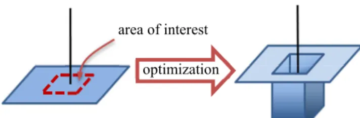
One solution is to find easily-constructed sequences such as sequences of the Small Set of Kasami or other spreading codes families [1] [2]. However it can be noticed that those sequences have a good Peak to Sidelobe Level (PSL) on the whole ambiguity function area. But in practice the Doppler frequency range can be much smaller than the bandwidth of the probing signal. For example, consider a L-band radar operating at a wavelength of 0.3 m. An airliner with a radial speed of 300 m/s gives a Doppler frequency of 2 kHz which is much smaller than the bandwidth of many MHz. Also depending on the signal duration it is not relevant to optimize the whole distance range. For example, assuming a radar instrumented range of 150 km, a pulse repetition interval of 10 ms induces an unambiguous distance range of 1500 km which is much more than the radar instrumented range of 150 km. Therefore we confine our attention on a small area of interest defined by the maximum Doppler frequency and the radar instrumented range; we expect to obtain better sidelobe level (Fig 1.).

According to this remark, another solution is to generate a sequence such that the ambiguity function is locally optimized. This kind of waveform design can be achieved by the use of cyclic algorithm, like the one introduced by Stoïca and He [3]. However this algorithm is based on the Singular Value Decompositions (SVD) of a large matrix with a complexity of

O(N3) (where N is the number of elements in the sequences).

But recent works [4] have shown the possibility to optimize the autocorrelation sidelobe energy by using an efficient gradient method which reduces the complexity to O(Nlog(N)). In this paper, we extend this approach to the local optimization of the ambiguity function of aperiodic or periodic complex sequences.

Fig. 1. Expected result on the ambiguity function after local optimization. II. GRADIENT METHOD FOR OPTIMIZING THE MATCHED

FILTERING RESPONSE IN PRESENCE OF A DOPPLER

A. Notations and Purpose

First, define a complex sequence of length

N, with and its Doppler shift version where and corresponds respectively to the Doppler shift and the bit time. is supposed to be the predefined waveform envelope (i.e. of constant modulus or pulsed etc.).

If we define a normalized Doppler shift such that then can be designed by !" . According to that, the correlation of and , expressed as

# $ , is given by: % & '

$

(₎*

+ $ _{, &} (1)

One important feature of this function is:

%$ _{& %- .&} ) _{/ 0} 12*345617819 : ; 7<=56>1?5 (2) Now let us define the energy term from which we calculate the gradient:

@ + A%B & A CD)

-) - E

(3) where the exponent F allows some control over the sidelobe level. When F G, @ corresponds to the weighted integrated sidelobe level. Otherwise, the larger the exponent, the more emphasized the dominant term is, so the gradient will essentially indicate the gradient of the PSL. The coefficients D) control the shape of the correlation sidelobes.

optimization area of interest

B. Gradient calculations

This subsection provides the gradient of @ . The details of the derivations for calculating this gradient are given in APPENDIX A. Therefore, for understanding and completeness, this part focuses on the key points of the gradient calculation.

As is a complex sequence with a predefined envelope, the gradient can be written as the derivative of the sidelobe energy @ with respect to its phase: H@_HI

J only.

But using the chain rule, it can be observed that the derivative with respect to the phase of can be done by calculating the derivatives with respect to the real and imaginary parts of : H@ HIK .LM K H@ HN K , N K H@ HLM K (4) H@ H O F + P)Q HA% & AH O -) - E (5) where P_)Q D₎A% & A C- and H O /HN K

HLM K , and as RSR N S , LM S , it can be derived that:

H@ H O TF + P)Q UN V% & W HN V% & W H O -) - E , LM V% & WHLM V% & W_{H O} X

(6)

Then it can be shown (APPENDIX A) that the partial derivatives with respect to N _K and LM _K are given by the equations (7) and (8): H@ HN K TF + P)Q YN Z% & J , & - K _[ -) - E , N \% & Z J . & K-) [$]^

(7)

H@

HLM K TF + P)Q YLM Z% & J , &

- K _[

-) - E

. LM \% & Z J . & K-) [$]^

(8)

Putting (7) and (8) into the chain rule equation (4) gives the equation (9). By defining _ `P_)Q a_{) - E}- and b / - c !d ) , the equation (9) becomes: H@ HIK .TFLM Y J eV'_ f # -# _{( $ ' f b (W} K , V'_ f # ( $ ' f b$(#W _{E -K}g^ (10) where h# i j , G . & ₎ the reverse of h, and f k is the Hadamard product of and k.

Then, by setting: l V'_ f #-# ( $ ' f b (W_K, V'_ f # ( $ ' f b$₍#_W E -K"K (11) and:

m

/

H@

_HI

K

d

_K (12)

Equation (10) can be converted to a vector form:

m

.TFLMn f l o

(13)

Finally the gradient can be expressed as a sum of correlation products that can be efficiently computed using Fast Fourier Transforms (FFT). If we denote by p *q the discrete Fourier Transform operation, it has been shown by Bracewell in

[5]

that a correlation in the time domain corresponds to product in the frequency domain. And according to our definition of the convolution (1), it can be derived that the convolution of two sequences h and r is equivalent to:

h $ r

p

.G_V

_{*p h p}

_'

_r

#$_{(W (14)} So that gives a computation of m

in

s jt7uj operations.

The algorithm follows naturally from the above discussion and it is summarized in Algorithm 1(see below)

Algorithm 1 : The gradient algorithm for minimizing the

matched filtering response in presence of a Doppler

Step 0 : Randomly initialize the phase of the sequence

Define the area of interestD₎ and (Doppler)

Step 1 : Gradient calculation: Determination of _

and

# for calculating*m vw_v

x"_K

.

Step 2 : Determination of the descent step y and update of

* :

- z{ Step 3 : Go to Step 1 until convergence

H@

HI_K .TFLM

|

J

} +

P&Q %. .&

Z

J , & .~T€ J,&j

[

$

, +

P_&Q % &

Z

J . & ~T€ J.&j

[

$ j.G & .j,G j.G & .j,G

•‚

(9)

III. GRADIENT METHOD FOR OPTIMIZING A SET OF DOPPLER EFFECTS ON THE AMBIGUITY FUNCTION

A. Notations and Purpose

In this section the gradient of the discrete ambiguity function sidelobe energy for a complex sequence is derived. This gradient is presented as an extension of the previous section for a set of Doppler.

If we call ƒ the set of Doppler frequency to optimize such that:

ƒ

R* : ;*12*45617819Q : „*7<=56>1?5

(15) Then, the energy term from which we calculate the gradient can be expressed as the sum of the partial energy for each Doppler in the set ƒ:

@ + @

:ƒ (16)

where we recall that:

@ + A% & A CD)Q

-) - E

(17) And D_)Q are the coefficients that allow controlling the shape of the correlation sidelobes for each Doppler in the set ƒ.

B. Gradient Calculations

According to the above discussion, it is obvious from (13) and (16) that the gradient expression is:

H@ HIK + H@ HIK :ƒ (18) Therefore by defining: m /_HIH@ Kd_K (19) it comes: m + m :ƒ (20)

Similarly to the previous section, the gradient consists on a sum of correlation products that can be efficiently computed using Fast Fourier Transforms (FFT)

[4].

So the computation of m can be done in s j…†‡j operations. The algorithm follows naturally from the above discussion and it is summarized in Algorithm 2.

IV. APPLICATIONS

This section provides some applications of those algorithms such as:

- The design of a complex sequence for optimizing the matched filter response in presence of Doppler in the periodic and aperiodic case.

- And the design of a complex sequence for optimizing the ambiguity function in the periodic and aperiodic case.

A. Optimizing both the response of the matched filter in presence of a Doppler and the autocorrelation of a complex sequence in the aperiodic and the periodic case

The following examples show the sidelobes rejection that can be obtained by an iterative application of (20) in Algorithm

2.

A random complex sequence is generated as a starting point for the algorithm and then a gradient descent is done by simply adjusting the descent step y during the process. The global gradient is calculated once in each iteration. This gradient corresponds to the sum on : ƒ of the partial gradient of @ . Therefore a number of ˆi%‰ ƒ partial gradients are calculated within the global gradient. Then the process continues until an exit criterion is met (an upper limit on the number of iterations, or a lower threshold on the minimum improvement acceptable between two successive iterations).

It is relevant to notice that the optimization of the response of the matched filter with a Doppler optimizes also the response of the matched filter with a Doppler Š (because (3)). Therefore it is sufficient to define ƒ such that:*ƒ ` R* : R* : ;E_{*12*45617819Q : „}E_{*7<=56>1?5 a or such} that ƒ is symmetric.

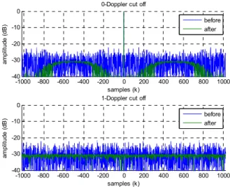
Figure (2) and Figure (3) show the improvement after optimizing the autocorrelation and one Doppler on the ambiguity function (ƒ ‹*Œ G ) of a complex sequence (of length j G‹T•) with a constant weighting (D_)Q GQ 0&*Q 0 ) and a large exponent (F •) in the aperiodic and periodic case, respectively.

On the other side, Figure (4) and Figure (5) represent the improvement after optimizing the autocorrelation and one Doppler on the ambiguity function (ƒ ‹*Œ G ) of a complex sequence (j G‹T•) for a local weighting (D_)Q GQ J R&R Ž T••*7<=56>1?5*‹Q 0 ) and a large exponent (F •) in the aperiodic and periodic case, respectively.

Algorithm 2 : The gradient algorithm for optimizing a set of

Doppler on the ambiguity function

Step 0 : Randomly initialize the phase of the sequence

Define the area of interest: the set of Doppler, ƒ and the weighting coefficients associated, D_)Q .

Step 1 : Gradient calculations for each Doppler: Determination of _

,

# and*m vw_v

x"_K for calculating*m _vvw

x"_K

.

Step 2 : Determination of the descent step y and update of :

- zm Step 3 : Go to Step 1 until convergence

Fig. 2. Matched filter response for a normalized Doppler ‹*Œ G ‘j in the aperiodic case: before (blue) and after (green) optimization.

Fig. 3. Matched filter response for a normalized Doppler ‹*Œ G ‘j in the periodic case: before (blue) and after (green) optimization.

Fig. 4. Matched filter response for a normalized Doppler ‹*Œ G ‘j in the weighted aperiodic case: before (blue) and after (green) optimization.

Fig. 5. Matched filter response for a normalized Doppler ‹*Œ G ‘j in the weighted periodic case: before (blue) and after (green) optimization.

TABLE I. PSL IMPROVEMENT OF EXAMPLE A

Aperiodic Periodic Weighted Aperiodic

Weighted Periodic

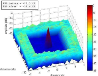
It is obvious on those examples that the minimization gives a good improvement on the PSL. And the smaller the optimization area is, the better the improvement is (the less the system is constrained) (See TABLE 1.)

B. Optimizing locally the ambiguity function of a complex sequence in aperiodic and periodic case

The following examples show the sidelobe rejection possible on the area of interest of the ambiguity function by an iterative application of (20) in Algorithm 2. As the previous examples, a random complex sequence is generated as a starting point for the algorithm. Then a gradient descent is done by simply adjusting the descent step y during the process. The global gradient is calculated once in each iteration and the process continues until an exit criterion is met (an upper limit on the number of iterations, or a lower threshold on the minimum improvement acceptable between two successive iterations).

Figure (6) and Figure (7) show the improvement after optimizing a set of Doppler on the ambiguity function (ƒ

‹*Œ G*Œ T*Œ ’ ) of a complex sequence (j G‹T•) with a constant weighting (D_)Q GQ 0&*Q 0 ) and a large exponent (F •) in the aperiodic and periodic case, respectively.

On the other side, Figure (8) and Figure (9) show the improvement after optimizing a set of Doppler on the ambiguity function (ƒ ‹*Œ G*Œ T*Œ ’ ) of a complex sequence (j G‹T•) with a local weighting (D_)Q GQ J R&R Ž GT“*7<=56>1?5*‹Q 0 ) and a large exponent (F •) in the aperiodic and periodic case, respectively.

-1000 -800 -600 -400 -200 0 200 400 600 800 1000 -40 -30 -20 -10 0 samples (k) a m p li tu d e ( d B )

0-Doppler cut off

before after -1000 -800 -600 -400 -200 0 200 400 600 800 1000 -40 -30 -20 -10 0 samples (k) a m p lit u d e ( d B )

1-Doppler cut off

before after -1000 -800 -600 -400 -200 0 200 400 600 800 1000 -40 -30 -20 -10 0 samples (k) a m p li tu d e ( d B )

0-Doppler cut off

before after -1000 -800 -600 -400 -200 0 200 400 600 800 1000 -40 -30 -20 -10 0 samples (k) a m p lit u d e ( d B )

1-Doppler cut off

before after -1000 -800 -600 -400 -200 0 200 400 600 800 1000 -50 -40 -30 -20 -10 0 samples (k) a m p lit u d e ( d B )

0-Doppler cut off

before after -1000 -800 -600 -400 -200 0 200 400 600 800 1000 -50 -40 -30 -20 -10 0 samples (k) a m p li tu d e ( d B )

1-Doppler cut off

before after -1000 -800 -600 -400 -200 0 200 400 600 800 1000 -50 -40 -30 -20 -10 0 samples (k) a m p lit u d e ( d B )

0-Doppler cut off

before after -1000 -800 -600 -400 -200 0 200 400 600 800 1000 -50 -40 -30 -20 -10 0 samples (k) a m p li tu d e ( d B )

1-Doppler cut off

before after

Fig. 6. Ambiguity function obtained when optimizing a set of Doppler ƒ ‹*Œ G*Œ T*Œ ’ ‘j on the whole distance range in aperiodic case

Fig. 7. Ambiguity function obtained when optimizing a set of Doppler ƒ ‹*Œ G*Œ T*Œ ’ ‘j on the whole distance range in periodic case

Fig. 8. Ambiguity function obtained when optimizing a set of Doppler ƒ ‹*Œ G*Œ T*Œ ’ ‘j on a weighted range profil in aperiodic case

Fig. 9. Ambiguity function obtained when optimizing a set of Doppler ƒ ‹*Œ G*Œ T*Œ ’ ‘j on a weighted range profil in periodic case

As we can see, the algorithm well-improves the PSL in the area of interest. As an example, for a sequence from the Small Set of Kasami, the PSL is about T‘”j; that corresponds to .T•*‰• for a sequence of 1024 elements [1]. So even compared to those easily-constructed sequences, our algorithm gives better result.

Moreover, this algorithm is highly faster than the cyclic algorithms introduced by Stoïca and He [3]. This is due to the efficient calculations of the gradient whereas cyclic algorithms are based on a SVD operation on each iteration.

V. CONCLUSION

In this paper, new gradient methods for optimizing complex sequences’ ambiguity functions were derived. We have shown that the gradient for optimizing the matched filtering response in presence of a Doppler is based on simple operations on a small number of correlations. We have also shown that the gradient for optimizing a set of Doppler on the ambiguity function is an extension of the previous one; therefore it is also based on simple correlation operations.

Since the correlation can be performed using Fast Fourier Transforms, the result is that the gradient can be computed with O(Nlog(N)) operations. This important result offers the possibility to optimize quite long sequences with a relatively short time of computation compared to existing methods.

Moreover, these algorithms optimize quite well the PSL in the area of interest using an adequate weighting. Therefore, they can be used for designing sequences for radar applications.

VI. APPENDIX A : ON GRADIENT CALCULATION DETAILS In this paper we have derived briefly the key points of the gradient calculations. Here, we give more details on those derivations.

As it has been discussed in the previous part, the gradient calculations consist on calculations of the derivative with respect to the real and the imaginary parts of

We recall that : H@ H O TF + P)Q UN V% & WHN V% & W_{H O} -) - E , LM V% & WHLM V% & W_{H O} X

(21)

whereP _Q) D _Q)A% & A C- and H O /HN K HLM K

So, for calculating vw_{v O}, we have to calculate v–—V˜_{v O} ) W* and v–—V˜ ) W

v O . Let us start with some developments on the real and imaginary parts of % & :

N V% & W N |+ $ _{, & ‚*} + N V $ _{, & W} ™JŒ* ™J.& , N Z J Z J , & - K _[$_[ , N Z $ _{J J . &} K-) _[ (22) LM V% & W LM |+ $ _{, & ‚*} + LM V $ _{, & W} ™JŒ* ™J.& , LM Z J Z J , & - K [$[ , LM Z $ _{J J . &} K-) _[ (23)

For two complex i and š, we have:

N iš N i N š . LM i LM š (24)

N iš$ _{N i N š , LM i LM š (25)}

LM iš LM i N š , N i LM š (26)

LM iš$ _{LM i N š . N i LM š (27)}

Hence the real and the imaginary parts of % & become:

N V% & W + N V $ _{, & W} ›KŒ* ›K-) , N ' J (N Z J , & - K _[ , LM' J (LM Z J , & - K _[ , N ' J (N Z J . & K-) [ , LM' J (LM Z J . & K-) [ (28) and : LM V% & W + LM V $ _{, & W} ›KŒ* ›K-) , LM' J (N Z J , & - K [ . N ' J (LM Z J , & - K _[ . LM' J (N Z J . & K-) [ , N ' J (LM Z J . & K-) [ (29)

It follows from (28) and (29) that: HN V% & W HN K N Z J , & - K _[* , N Z J . & K-) [ (30) HLM V% & W HN K .LM Z J , & - K _[* , LM Z J . & K-) [ (31) HN V% & W HLM K LM Z J , & - K _[* , LM Z J . & K-) [ (32) HLM V% & W HLM K N Z J , & - K _[* . N Z J . & K-) [ (33)

And by combining (21), (24)-(27) and (30)-(33), it comes: H@ HN K TF + P)Q YN Z% & J , & - K _[ -) - E , N \% & Z J . & K-) [$]^ (34) H@

HLM K TF + P)Q YLM Z% & J , &

- K _[ -) - E . LM \% & Z J . & K-) [$]^ (35)

œ

REFERENCES

[1] F. Arlery, M. Klein et F. Lehmann, «Utilization of Spreading Codes as dedicated waveforms for Active Multi-Static Primary Surveillance Radar,» IEEE Radar Symposium (IRS), pp. 327-332, 2015.

[2] D. V. Sarwate et M. B. Pursley, Crosscorrelation properties of pseudorandom and related sequences, vol. 68, Proceeding of the IEEE, Mai 1980, pp. 593-619.

[3] H. He, J. Li et P. Stoica, Waveform Design for Active Sensing Systems : A Computational Approach, New York: Cambridge University Press, 2012.

[4] J. M. Baden, M. S. Davis et L. Schmieder, «Efficient Energy Gradient Calculations for Binary and Complex Sequences,» RadarCon, pp. 301-309, Mai 2015.

[5] R. N. Bracewell, The Fourier Transform and its Applications, 3rd Edition éd., New York: McGraw-Hill, 1986.