HAL Id: hal-01847589
https://hal.archives-ouvertes.fr/hal-01847589
Submitted on 6 Nov 2018
HAL is a multi-disciplinary open access
archive for the deposit and dissemination of
sci-entific research documents, whether they are
pub-lished or not. The documents may come from
teaching and research institutions in France or
abroad, or from public or private research centers.
L’archive ouverte pluridisciplinaire HAL, est
destinée au dépôt et à la diffusion de documents
scientifiques de niveau recherche, publiés ou non,
émanant des établissements d’enseignement et de
recherche français ou étrangers, des laboratoires
publics ou privés.
A practical method to derive sample temperature during
nonisothermal coupled thermogravimetry analysis and
differential scanning calorimetry experiments
Sylvain Salvador, Jean Henry Ferrasse
To cite this version:
Sylvain Salvador, Jean Henry Ferrasse.
A practical method to derive sample temperature
dur-ing nonisothermal coupled thermogravimetry analysis and differential scanndur-ing calorimetry
ex-periments.
Chemical Engineering and Technology, Wiley-VCH Verlag, 2006, 29 (6), p.696-702.
A Practical Method to Derive Sample Temperature during
Nonisothermal Coupled Thermogravimetry Analysis and
Differential Scanning Calorimetry Experiments
By Sylvain Salvador and Jean-Henry Ferrasse*
Nonisothermal thermogravimetry differential scanning calorimetry (TG-DSC) mounting is intensively used for the determi-nation of kinetic parameters and reaction heat along the chemical transformation of a solid. Nevertheless, when tests are per-formed with heating rates as high as those encountered in industrial processes, e.g., several tens of K min–1, there is great
un-certainty in the knowledge of the exact sample temperature. In this work, a method to derive a simple mathematical expres-sion is proposed and fully described in order to calculate the real sample temperature throughout a temperature-ramped test on a commercial apparatus. The furnace temperature and the heat flow signals were used, together with the crucible specific heat and the heating rate. A number of validation tests were performed to derive similar reaction rates for a reference. First-order kinetic reactions were presented and reconciled over a large range of heating rates from 3 to 50 K min–1.
1 Introduction
Temperature-ramped thermogravimetry (TG) analysis is an efficient way to derive, from a single experiment, kinetic parameters for chemical reactions such as thermal degrada-tion over a wide range of temperature. Coupling mass infor-mation to heat flow inforinfor-mation additionally facilitates the derivation of the reaction heat associated with the transfor-mation (differential scanning calorimetry (DSC)). For technical reasons, it is difficult in coupled TG-DSC mount-ings to measure the sample temperature while weighing it continuously with high precision. The temperature is, therefore, usually measured from a thermocouple placed either inside the atmosphere gas or inserted into the furnace wall. However, it is established that there can exist a temper-ature gap between the furnace and the crucible as high as several tens of degrees. This causes a problem since the rele-vant temperature for kinetic parameter determination is the sample temperature [1]. High heating rates favor this differ-ence.
A number of technical procedures have been proposed to solve this problem. They are mainly based on different ex-periments, one for mass recording and some others for
tem-perature recording [2, 3]. Subramanian [4] proposed a mounting with optical measurement of temperatures, with-out direct contact of the probe with the crucible. The effect of emissive properties of materials now needs to be investi-gated more thoroughly to check the reliability of measure-ments.
In contrast to purely technical solutions, some authors tried mathematical corrections. Sigrist [5] developed a black-box type of model for the heat flowmeter crucible mounting. The author proposes an apparatus transfer func-tion that links melting points of standards (inputs) with the recorded signals during experiments (outputs). The author, nevertheless, notices himself that the apparatus function var-ies according to the data set used to calculate them. Dong et al. [6] proposed a numerical model using enthalpy as a func-tion of temperature as an input. A temperature is then scanned or modulated. The response of the calorimeter is calculated. This predicts the sample thermocouple tempera-ture and the temperatempera-ture difference between the sample and reference thermocouples as a function of time and tempera-ture.
In this paper, a practical method is proposed for establish-ing a simple mathematical expression dedicated to the TG-DSC apparatus used, to calculate throughout an experiment the temperature difference, TD, between the sample and the furnace. The method is based on a description of the net heat flow recorded as the sum of a crucible inertia heat flow, a sample inertia heat flow, and a chemical reaction heat flow. The expression is determined from a heat balance over the heat flowmeter, on the one hand, and from a heat balance over the crucible, on the other hand. A simplified heat trans-fer model is used. As detailed below, it is possible to fit the parameters appearing in the mathematical expression through the reconciliation of the kinetic parameters deter-mined at two different heating rates for a reference chemical reaction.
–
[*] Pr S. Salvador, Laboratoire de Génie des Procédés des Solides Divisés, Ecole des Mines d’Albi-Carmaux, UMR CNRS 2392, Campus Jarlard, route de Teillet, 81013 Albi CT CEDEX 09, France; Dr. J.-Henry Ferrasse (author to whom correspondence should be addressed, [email protected]), LMNSMGP, UMR CNRS 6181, Université Paul Cézanne d’Aix Marseille 3, Bâtiment Laennec, Hall C, Domaine du Petit Arbois, RD 54 BP, Avenue Louis Philibert, 13545 Aix en Provence Cedex 04, France.
2 Deriving Mathematical Expression
2.1 SETARAM TG-DSC 111 Mounting
The general arrangement of the TG-DSC coupling system used is shown in Fig. 1 (for details, see manufacturer (www.setaram.com)). A similar mounting is placed beside the one represented here (sample mounting), and generally operates with an empty crucible or a reference material (reference mounting). The recorded signals are the tempera-ture measured inside the furnace wall, Tf, the crucible plus
sample mass, mC+ mS, and the raw heat flow, !R-REC. As
detailed further, this flow signal is the difference between the sample heat flow thermopile signal, !R, and the
refer-ence heat flow thermopile signal, !REF.
2.2 Assumptions
a) It is assumed that the temperature of the crucible and the temperature of the sample remain identical and equal to
TC. For a detailed calculation based on the thermal Biot
number, the reader can refer to [7].
b) Convection heat transfer between the crucible and the furnace is generally supposed to be more efficient than radiation as long as the temperature remains below ap-proximately 500 °C. This was confirmed with the calcula-tion of the global heat transfer coefficient (see annex 1). c) For the low gas flow rates typically used, the flow inside
the furnace is laminar. The heat exchange between the crucible and the furnace can be described as heat conduc-tion through the atmosphere gas film that separates them. The validity of this assumption is stated (see also annex 1). Indeed, the Nusselt number for cocylindrical flow only depends on the diameter ratio and wall boundary [8]. d) The heat flowmeter presents a pure time delay, e.g., its
flow signal is time delayed, by sHFM seconds, as
com-pared with the actual heat flow leaving the crucible [9].
2.3 Mathematical Modeling
The mathematical modeling is only based on several en-thalpy balances.
The enthalpy balance for the flowmeter (domain F in Fig. 1) gives1):
!R! M# D" Ms$dTdt "c !Ch" !g (1)
where !Ris the raw heat flow (measured by the sample
ther-mopile), the first term on the right-hand side is the thermal inertia of the crucible + sample, !Chis the chemical reaction
heat flow, and !gis the heat flow resulting from the enthalpy
variation of the sweeping gas entering and leaving the domain. The term !gis suppressed by running a blank test in
which an empty crucible is heated under the same tempera-ture ramp. During this blank test, the heat flow of the sam-ple thermopile can be expressed as:
!B= MCb+ !g (2)
In Eqs. (1) and (2), !g can be considered as equal. It
should be borne in mind that an error might be introduced by the fact that the total exit gas flow changes when some gas is produced by the reaction. With the assumption made above, the heat flow due to the product gas enthalpy is incor-porated into !Ch.
The flow signal recorded by the apparatus, !R-REC, is the
difference between the sample thermopile signal !Rand the
reference thermopile signal !REF. Thus, the recorded raw
signal is:
!R-REC= !R– !REF
Figure 1. Arrangement of TG-DSC apparatus. (1) crucible, (2) sample, (3)
thermopile, (4) furnace, (5) atmosphere gas, (6) heating elements, (7) weigh-ing system, (8) furnace thermocouple. A similar mountweigh-ing (reference cruci-ble) is located beside this one.
–
and the recorded blank signal is: !B-REC= !B– !REF
Substracting the recorded blank flow !B-RECfrom the
re-corded raw flow !R-RECgives the “recorded” net flow:
!N-REC! !R-REC% !B-REC! M# C" Ms$dTdt "c !Ch% MCb
(3) since the reference flow signal !REFis the same during the
experiment and during the blank test.
An enthalpy balance for the crucible + sample (domain C in Fig. 1) gives:
MC" Ms
# $dTdt "c !Ch% !C-F ! 0 (4)
where !C-Fis the exchanged flow between the crucible and
the furnace.
Following assumption (c), the term !C-Fwill be expressed
as:
!C-F= Akf(TW– TC) (5)
where A is a constant that characterizes the TG-DSC appa-ratus under the atmosphere flow conditions used, and kf is
the thermal conductivity of the atmosphere gas. In the fol-lowing, this conductivity will be assessed as a polynomial function of the furnace temperature. Eq. (5) shows that there exists a temperature difference due to heat transfer,
TDHT, between the crucible and the furnace. This difference
can be expressed from Eqs. (3), (4), and (5): TDHT!!N-RECA k" Mcb
f (6)
In addition, the heat flow measurement system globally introduces a response time sHFM(see assumption (d)) which
will be responsible for another temperature difference be-tween the crucible and the furnace, TDHFM [9]. This term
can be expressed from the flowmeter time delay sHFMand
from the heating rate b:
TDHFM= sHFMb (7)
Thus, the total temperature difference between the cruci-ble and the furnace is:
TD = Tf– Tc= TDHT+ TDHFM (8)
Moreover, the chemical reaction heat flow can be ex-pressed as follows if the reaction heat DH is in J kg lost–1:
!Ch ! dmdtS DH (9)
Finally, the net recorded flow can be rewritten from Eqs. (3) and (9):
!N%REC! M# C" Ms$dTdt "c dmdtS DH % MCb
(10) In Eq. (10), it appears that the net recorded flow is the sum of three separate heat flows. The method consists in cal-culating each of these flow contributions and in summing them to calculate a net flow !N-c. The unknown parameters
(DH, cp, A) are determined by fitting !N-RECand !N-con a
standard experiment.
Then, TD can be calculated by adjusting sHFMwith a
sec-ond standard experiment.
2.4 Experiments
In the proposed method, the standard experiments are conducted with a reference material. 30 mg of calcium oxalate are heated at 3 K min–1 (first experiment) and
30 K min–1 (second experiment) under a nitrogen
atmo-sphere; the flow rate is 54 mL min–1at STP conditions.
In the temperature range from 150 to 350 °C, calcium oxa-late undergoes a decomposition to carbonate, responsible for approximately 12 % mass loss. The reaction heat is reported as –400 kJ kg oxalate–1, which is equivalent to
3.33 MJ kg lost–1.
3 Validation of the Model
3.1 Determination of Constants in Expression of TD
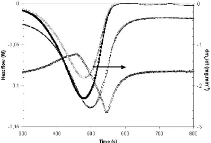
The recorded net heat flow !N-RECand the DTG signal
(derived directly from the mass signal by the apparatus soft-ware) are plotted in Fig. 2; they reveal a time shift of ap-proximately 20 s between the peak values of the two signals. According to Eq. (9), the time shift between the two signals
Figure 2. Time evolution for oxalate of (+) the recorded net heat flow !N-REC
(W), (×) the sample mass derivative, (–) the calculated net heat flow !N-c
(W), (!) the chemical reaction heat flow !Ch(W), (") the crucible + sample
inertia heat flow (MC+ MS)dTC/dt (W), (...) arbitrary base line for heat
is physically unsatisfactory, confirming that !N-RECincludes
inertia terms. It is also possible to calculate and to plot in Fig. 2 two of the three terms on the right-hand side of Eq. (10) since:
– If A is fixed (initialization), the crucible temperature can be calculated from Eq. (6). MCis known; MScan be
calcu-lated from the sample mass mSrecorded during the test, if
cpSif fixed (initialization). The first term can then be
cal-culated.
– The chemical reaction heat, the second term in Eq. (10), can be calculated if a reaction heat DH is fixed.
– For the third term, the thermal inertia of the crucible is a known constant.
A problem may arise due to the fact that three unknowns are to be fitted: A, DH, and cpS. Nevertheless, they can be
determined through a series of easy trials and adjusted for the three terms. Indeed:
– When the chemical reaction is over, the net flow !N-cis
sensitive only to cpS. This specific heat is directly
deter-mined by fitting !N-cand !N-RECin the pre- or
postreac-tion zone, which is a common way of measuring specific heat when no reaction occurs.
– DH acts on the peak intensity of !N-cand on the left-right
position of the peak.
– A only acts on the left-right position of the !N-cpeak.
It is, therefore, possible to fix DH, A, and cpSseparately.
Several iterations lead to the !N-ccurve in Fig. 2, deriving
the values:
A= 0.140 m DH= –3.76 MJ kg–1
cpS= 1100 J kg–1K–1
These values could be fitted without ambiguity within ±2 %. The experimental net flow !N-RECwas satisfactorily
reconstructed from the sum of the three terms in Eq. (10) (see Fig. 2).
It is noteworthy that the inertia heat flow of the cruci-ble + sample is important as compared with the chemical re-action heat flow !Ch, which makes it important to run a high
quality blank test. Calculating MCand MSindicates that the
sample is responsible for only approximately 1 % of the total inertia.
Concerning oxalate, it is assumed that the chemical reac-tion follows first-order kinetics. It is then possible to calcu-late the reaction rate k at each temperature from Eq. (11) since dm/dt and m are known:
dm
dt ! %k m ! % A0exp%
E
R T m (11)
where m is the reactive remaining mass, or ms– mfinal.
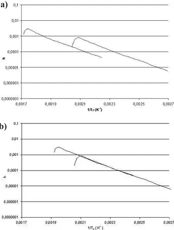
The values of k along the test performed at 30 K min–1,
and those for the test performed at 3 K min–1, using the
fur-nace temperature in the abscissa (1/Tf) are plotted in
Fig. 3a). The plot exhibits straight lines, which indicates that the first-order kinetics is a suitable model to describe the reaction. Nevertheless, large differences in values of k for a given temperature are observed, due to the error introduced
by the use of the furnace temperature instead of the actual sample temperature. As !N-cis not sensitive to sHFM, (that
appears only in Eq. (7)), it is possible to completely recon-cile the reaction rates obtained at two heating rates (see Fig. 3b)), using a value of 12.0 s for sHFM.
The temperature correction that finally has to be applied is:
TD ! Tf% Tc!!N-REC0!140 k" Mcb
g " 12!0 b (13)
The temperature difference TD of the crucible towards the furnace during the two experiments can reach a value as high as 35 °C during the test at 30 K min–1. The TD during
the test at 3 K min–1is much lower but still not negligible. It
has to be noticed that, assuming the chemical reaction heat flow !Chis set equal to zero, TD significantly decreases with
increasing furnace temperature, this being only due to the increase in kfwith temperature.
3.2 Validation of Method
At first, the constants determined through the procedure have a physical meaning:
a)
b)
Figure 3. Reaction rate for decomposition to carbonate of calcium oxalate
re-action during experiments with heating rates of (–) 3 K min–1 and (–)
30 K min–1. (a) Abscissa is 1/T
– The calculated chemical reaction heat flow signal !Chis
time-synchronized with the mass derivative, which satisfies the basic physical concept of reaction heat in Eq. (9). – The reaction heat derived is equal (within the fitting error,
or±2 %) to that given by the classical integration of the surface between the net flow curve !N-RECand the base
line represented in Fig. 2.
– The value of 1100 for the sample-specific heat cpSis a
suit-able value.
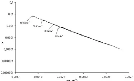
To check the validity of the calculation of TD, two addi-tional tests with heating rates of 15 and 50 K min–1were
per-formed. In Fig. 4, the values of the reaction rate k from the experiments at 3, 15, 30 and 50 K min–1were plotted versus
the reverse of the crucible temperature calculated using the expression of TD in Eq. (13). Whatever the heating rate operated, the values of k are very similar; this attests for the good description of TD.
Finally, another validation test was performed with potas-sium perchlorate. This calibration material is reported to un-dergo a transition at the reference temperature of 300 °C. The transformation occurs without mass change of the sam-ple. The product was heated at 30 K min–1, under a
54 mL min–1flow of N
2. Fig. 5 illustrates the evolution of the
furnace temperature and that of the crucible, calculated using the expression of TD derived previously. The net recorded heat flow has also been plotted. It is generally ad-mitted that the period where a transition occurs or where the smelting of a metal is isothermal, is the period during which the heat flow curve is linear. This zone is indicated in the figure thanks to two vertical dotted lines. During this period, the calculated temperature of the crucible indicates a plateau around 305 °C. This value is very close to the refer-ence temperature of 300 °C, while, during the same period, the furnace temperature is between 325 and 332 °C. The correction using TD appears to give a much better estimation of the actual sample temperature.
4 Conclusion
It is possible to derive a simple mathema-tical expression to calculate the actual cruci-ble. This expression requires the recorded net heat flow data and the heating rate as in-puts plus a number of constants that charac-terize the TG-DSC mounting, whose meth-od of determination has been detailed. This determination necessitates conduction of two simple experiments with different heat-ing rates, and a simple posttreatment of the data in a series of manual trials to adjust four parameters whose independence has been checked. For clarity, the procedure is summarized in the appendix.
The method can be generalized to other TG-DSC mountings in which the crucible is separated from the heating source by an air film. In the case of the apparatus used here and a standard 5 mm outer diameter plati-num crucible, the expression for the temper-ature difference between the crucible and the furnace is:
TD ! Tf% Tc ! !N-REC0!140 k" Mcb
g " 12!0 b
where !N-REC is the blank corrected heat
flow and b the heating rate.
The decomposition of the net heat flow into a sum of identified heat flows also has the advantage of leading to the determina-tion of the reacdetermina-tion heat and of the sample specific heat. This and other considerations
Figure 4. Reaction rate for monoxide release from calcium oxalate reaction during experiments
with heating rates of 3, 15, 30, and 50 K min–1versus sample corrected temperature.
Figure 5. Temperature of furnace (–) and calculated temperature for crucible (–) during transition
reaction of potassium perchlorate, under nitrogen, at 30 K min–1. (–) Net recorded heat flow
enable the physical meanings to be ascribed to the derived mathematical expression.
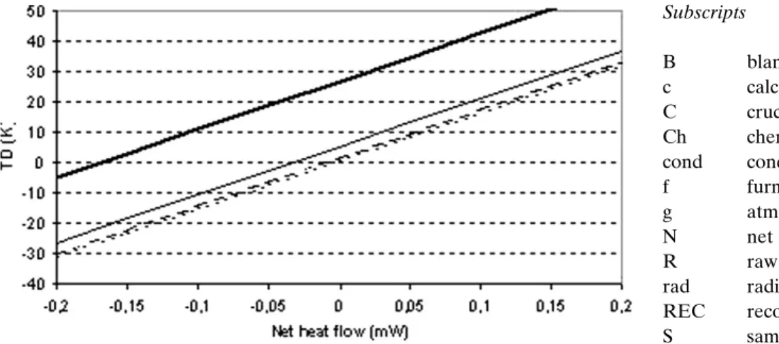
For practical purposes, Fig. 6 established from the mathe-matical expression gives the temperature difference between the crucible and the furnace as a function of the net heat flow (given by the apparatus along an experiment) for differ-ent heating rates. It confirms the necessity in most of the cases to operate a furnace temperature correction such as the one studied here.
Finally, for oxalate, it is shown that the expression of TD to calculate the sample temperature allows derivation of similar reaction rates for a first-order kinetic reaction over a wide range of heating rates: 3 to 50 K min–1.
Received: January 17, 2006
Symbols used
A [m] apparatus constant cp [J kg–1K–1] specific heat D [m] diameter k [s–1] reaction rate l [m] height of crucible m [kg] mass M [J K–1] heat capacity = m*cp S [m2] surface T [K] temperature TD [K] temperature difference Greek letters ! [W] heat flow b [K s–1] heating rate k [W m–1K–1] thermal conductivity e [–] emissivitys [–] characteristic time constant DH [J kg–1] chemical reaction heat
Subscripts B blank c calculated C crucible Ch chemical reaction cond conduction f furnace g atmosphere gas N net R raw rad radiation REC recorded S sample HT heat transfer HFM heat flowmeter W wall’s furnace
This paper’s data mc= 9.66 10–4kg
cpC= 133 J kg–1K–1
Sc= 1.770 10–4m2(crucible belt + bottom)
eC= 0.25
ef= 0.3
References
[1] C. David, S. Salvador, J. L. Dirion, M. Quintard, J. Anal. Appl. Pyrol.
2003, 67 (2), 307.
[2] I. Milosavljevic, V. Oja, V. Suuberg, Ind. Eng. Chem. Res.1996, 35, 653.
[3] J. A. Conesa, A. Marcilla, R. Moral, J. Moreno-Caselles, et al.,
Thermo-chim. Acta1998, 313, 63.
[4] J. S. Subramanian, P. K. Gallagher, Thermochim. Acta1995, 269/270, 89.
[5] K. Sigrist, P. K. Stach, Thermochim. Acta1996, 278, 145.
[6] P. K. Dong, P. K. Hunt, in Proc. of the 14thSymp. on Thermophysical
Properties, Boulder, CO, USA,2000.
[7] J. H. Ferrasse, Ph.D. Thesis, Ecole des Mines d’Albi-Carmaux, France
2000.
[8] F. P. Incropera, D. P. DeWitt, Fundamentals of Heat and Mass Transfer, 4thed., John Wiley & Sons, New York1996.
[9] E. Calvet, H. Prat, Microcalorimétrie. Applications Physico-Chimiques
et Biologiques, Masson & Cie, Paris1956.
[10] R. Siegel, J. R. Howel, Thermal Radiation Heat Transfer, 3rded., Taylor
& Francis, London1992.
Appendix
Summary of the procedure
●Run two experiments with 30 mg of calcium oxalate under
nitrogen at 3 and 30 K min–1.
●Run the blanks.
●Calculate the recorded net heat flows !N-REC (classical
correction of an experiment with a blank test).
●Plot on the same graph !N-REC for the experiment at
30 K min–1and !
N-c, sum of the terms on the right-hand
side of Eq. (10), e.g.:
Figure 6. General plot of temperature difference TD between furnace and crucible (-) versus
re-corded net heat flow !N-RECduring any experiment with a heating rate of (...) 1; (- -) 3; (-) 10, and
(-) 50 K min–1. The curves are established for a SETARAM TG-DSC 111 apparatus with the
– M# C" Ms$dTdtc where dTdtc is obtained deriving numeri-cally TC. with TC= TF– TD where TD ! TDHT " TDHFM ! !N-RECA k" Mcb g " sHFMb
in which A, cpS(in MS), and sHFMare initialized (see
re-sults presented in this paper);
– !Ch ! dmSdt DHin which DH is initialized;
– MCbis a known constant.
●Adjust cpS, A and DH to fit with !N-cand !N-REC.
●Plot on the same graph the values of k versus 1/TC(see
Fig. 3(b)) for the two experiments at 3 and 30 K min–1,
(TC= Tf– TD).
●adjust sHFMto reconcile the two curves for k.
The expression
TD ! Tf % Tc ! !N-RECA k" Mcb
g " sHFMb
is fully determined.
Annex 1
To calculate the equivalent heat transfer coefficient at the surface of the crucible h, the resistance between the crucible and the surroundings can be expressed as follows, using the crucible outside surface Sc(wall + bottom):
RC%f ! 1
h Sc (16)
The two expressions of the resistance in Eqs. (15) and (16) lead to h = 31.5 W m–2K–1.
The validity of the assumption of conductive heat transfer between the crucible and the furnace wall was checked by running an experiment at 30 K min–1 with a different N
2
flow: 20 mL min–1at STP conditions. The value of constant
Afitted from this experiment was again 0.14. The fact that the heat transfer coefficient does not depend upon the flow
velocity attests for the mainly conductive – and not convec-tive – nature of the heat transfer.
The contribution of radiation to the heat exchange be-tween the crucible and the furnace wall can be estimated at this stage. The global heat transfer coefficient h can be expressed as the sum of a conduction heat transfer hcondand
of a radiation heat transfer hrad:
h= hcond+ hrad (17)
The value of hradcan be estimated from the following two
expressions of the radiative heat flow between the furnace and the crucible:
efecr T! f4% Tc4"! hrad!Tf% Tc4" (18)
where the emissivities efand efare taken from [10], and r is
the Boltzmann constant. At the reaction peak, for instance, the furnace temperature is Tf= 275 °C and the crucible
tem-perature is Tc= 311 °C. This gives a value for hrad of
3.09 W m–2K–1. This shows, by comparison with the global
heat transfer coefficient h = 31.5 W m–2K–1, that the
contri-bution of radiation in this range of temperature is small. As far as the heat transfer between the crucible and the furnace is concerned, a reference can be found in terms of the equivalent conduction resistance to cross the atmosphere gas film separating the crucible and the furnace wall. This re-sistance can be expressed in cylindrical geometry:
Rcond ! 2 p k1 fl ln
Df
DC (14)
At the reaction peak intensity, for example, where
Tf= 275 °C and kf= 0.0436 W m–1K–1, its value is 143 K W–1.
On the other hand, Eq. (5) is equivalent to:
R ! A k1
f (15)
With the fitted value A= 0.140, this gives R = 164 K W–1.
The similarity in the values of R and Rcond attests for the