HAL Id: tel-02062224
https://tel.archives-ouvertes.fr/tel-02062224
Submitted on 8 Mar 2019HAL is a multi-disciplinary open access archive for the deposit and dissemination of sci-entific research documents, whether they are pub-lished or not. The documents may come from teaching and research institutions in France or abroad, or from public or private research centers.
L’archive ouverte pluridisciplinaire HAL, est destinée au dépôt et à la diffusion de documents scientifiques de niveau recherche, publiés ou non, émanant des établissements d’enseignement et de recherche français ou étrangers, des laboratoires publics ou privés.
Reeb Graph Modeling of 3-D Animated Meshes and its
Applications to Shape Recognition and Dynamic
Compression
Meha Hachani
To cite this version:
Meha Hachani. Reeb Graph Modeling of 3-D Animated Meshes and its Applications to Shape Recog-nition and Dynamic Compression. Networking and Internet Architecture [cs.NI]. Université Mont-pellier; École nationale d’ingénieurs de Tunis (Tunisie), 2015. English. �NNT : 2015MONTS152�. �tel-02062224�
Université Tunis El Manar
B.P. 37 le Belvédère 1002 Tunis Tunisie ب ص 37 رادــفلبلا1002 ســنوـــت Tél. : 216 71 874 700 /71 875 475 فتاهلا: Fax : 216 71 872 729 : سكافلا
Email : Enit@ enit.rnu.tn ينوتكللإا ديربلا:
THÈSE
Présentée pour obtenir le titre de
DOCTEUR
DE L’ÉCOLE NATIONALE D’INGÉNIEURS DE TUNIS
SPÉCIALITÉ : TÉLÉCOMMUNICATIONS
Par
Meha Hachani
Le 19 décembre 2015
Reeb Graph Modeling of 3-D Animated Meshes and
its Applications to Shape Recognition and Dynamic
Compression
Pr. Taoufik AGUILI (Sys’Com-ENIT) Pr. Amel BEN AZZA (Sup’Com)
Pr. Mohamed DAOUDI (Télècom-Lille1) Pr. Gilles GESQUIERE (UL-LYON2)
Président Rapporteur Rapporteur Examinateur
Pr. Azza OULED ZAID (Sys’Com –ENIT)
Pr. William PUECH (LIRMM- UM)
Directeur de thèse
Co-directeur de thèse
Acknowledgements
The three-year thesis are achieved only with the efforts deployed by my advisors. Now I’ve had the opportunity to express the deepest appreciation to my two thesis supervisors for their support, encouragement and more specifically for having made me discover scientific research. During these three years, Pr. Azza Ouled Zaid (Professor at ENIT/Tunis) has been a scientific research guide. Thanks to her I have learned to properly present my research articles. I thank him for his support and the attention that she carried me. I would like to thank also Pr. William Puech (Professor at UM/ Montpellier) for his outstanding human qualities and its encouragements. I thank him also for his help and support to integrate and fit into the lab team during my internships at LIRMM laboratory.
Especial thanks to the reviewers of my manuscript for having accepted this significant task (over a short period) Pr. Mohamed Daoudi (Professor at Telecom lille1) who accepted to review my manuscript despite his time consuming respon-sabilities and Pr. Amel Ben Azza (Professor at SupCom/ Tunis) who also kindly accepted to sacrifice his precious time for reviewing my manuscript. I would like to thank the committee member Pr. Gilles Gesquière (Professor at Lyon 2 University) has agreed to participate in this jury as an examiner. My sincerest thanks go to Pr. Taoufik Aguili (SysCom resarch laboratory Director) who made me the honor of be-ing president of the committee. I’m sincerely grateful for all the commitee members. Fiannaly, I would like to thank my research colleagues at SysCom/ Tunis laboratory and LIRMM/ Montpellier for all the technical exchanges, scientific and their sympathy. Especial thanks to my team member ICAR at LIRMM laboratory for all the good memories that I have shared with them.
iii
Résumé en Français
Le développement fulgurant de réseaux informatiques, a entraîné l’apparition de diverses applications multimédia qui emploient des données 3D dans des multiples contextes. Si la majorité des travaux de recherche sur ces données s’est appuyées sur les modèles statiques, c’est à présent vers Les modèles dynamiques de maillages qu’il faut se tourner. Les séquences de maillages variant au cours de temps représentent un nouvel axe de recherche où leur analyse joue un rôle incontournable, tel que la compression, l’indexation ou encore l’extraction des squelettes.
Les formes dynamiques 3D sont généralement représentées par une séquence de maillages 3D avec une connectivité constante et une information temporelle fournie par une géométrie variable dans le temps. Cette représentation est soumise à une grande variété d’opérations de traitement telles que l’indexation, la segmen-tation et la compression. Cependant, le maillage triangulaire est une représensegmen-tation extrinsèque, sensible face aux différentes transformations affines et isométriques. Par conséquent, il a besoin d’un descripteur structurel intrinsèque avant d’être traité par l’une des opérations de traitement mentionnées ci-dessus. Pour relever ces défis, nous nous concentrons sur la modélisation topologique intrinsèque basée sur les graphes de Reeb. Un graphe de Reeb est une représentation graphique, de type squelette, décrivant la structure topologique du modèle 3D. Leurs constructions reposent sur la théorie de Morse, qui définit une fonction continue sur la surface fermée de l’objet. Cette fonction continue permet la segmentation de la surface de l’objet en régions, chaque région est représentée par un nœud. Les nœuds dont les régions associées sont connexes sont liés par une arête. Il existe différentes fonctions continues qui peuvent être utilisées pour la construction du graphe de Reeb des maillages triangulaires.
Représentation par graph de Reeb basée sur la diffusion de la chaleur Dans le cadre de notre travail, notre principale contribution consiste à définir une nouvelle fonction continue basée sur les propriétés de diffusion de la chaleur. Ce dernier est calculé comme la distance de diffusion d’un point de la surface aux points localisés aux extrémités du modèle 3D qui représentent l’extremum locales de l’objet (points caractéristiques) qui sont détectés en utilisant la notion de propagation de la chaleur. La restriction du noyau de la chaleur au domaine temporel rend la fonction proposée intrinsèque et stable contre les perturbations. Les résultats expérimentaux obtenus sur des modèles 3D dynamiques ont dé-montré la robustesse et l’efficacité de la fonction scalaire proposée. Cette approche de construction de graph de Reeb peut être extrêmement utile comme descripteur de forme locale pour la reconnaissance de forme 3D. Il peut également être introduit dans un système de compression dynamique basée sur la segmentation. Dans ce contexte, nous exploitons les graphes de Reeb dans deux applications largement
iv
utilisées qui sont la reconnaissance des formes et la compression dynamique 3D. Application à la reconnaissance de forme 3D
Dans une deuxième partie, nous avons proposé d’exploiter la méthode de construction de graphe de Reeb dans un système de reconnaissance de formes 3D non rigides. L’objectif consiste à segmenter le graphe de Reeb en cartes de Reeb définis comme cartes de topologie contrôlée. Chaque carte de Reeb est projetée vers le domaine planaire canonique qui peut être soit un disque unitaire ou un anneau unitaire selon le type de la carte. Ce dépliage dans le domaine planaire canonique introduit des distorsions d’aire et d’angle. En se basant sur une estimation de distorsion, l’extraction de vecteur caractéristique est effectuée. Nous calculons pour chaque carte un couple de signatures, qui sera utilisé par la suite pour faire l’appariement entre les cartes de Reeb. Pour évaluer l’efficacité de la fonction scalaire utilisée et les signatures proposées, nous avons testé cette méthode sur la base de données la plus connue SHREC 2012 contenant 1200 modèles 3D répartis en 60 classes. Les performances de notre technique ont été évaluées par le calcul de cinq scores : First Tiers, Second Tiers, Les k-meilleurs scores, la mesure E et le gain cumulé. La courbe précision/rappel a montré la capacité de la méthode à retrouver les classes d’objets, il s’agit d’un calcul statistique sur la base de données. Pour effectuer une comparaison fidèle avec d’autres méthodes de l’état de l’art, nous avons testé notre technique de reconnaissance de forme sur plusieurs bases de données tels que : SHREC 2010, SHREC 2011 et MCGill. D’après l’étude expérimentale sur ces bases de données, il a été montré que notre technique donne des résultats satisfaisants du point de vue compromis efficacité et rapidité par rapport aux techniques de l’état de l’art.
Applications à la compression dynamique basée sur la segmenta-tion
Dans une troisième partie, nous avons proposé de concevoir une technique de segmentation, des maillages dynamiques 3D. Cette technique de segmentation est basée sur la même notion de théorie de Morse et de graphe de Reeb. L’idée princi-pale est de détecter les nœuds critiques, en appliquant une analyse topologique des fonctions lisses définies sur la surface de maillage 3D. Le processus de segmentation est effectué en fonction des valeurs de la fonction scalaire proposée dans la première partie. Le principe consiste à dériver une segmentation purement topologique qui vise à partitionner le maillage en des régions rigides tout en estimant le mouvement de chaque région au cours du temps. Pour obtenir une bonne répartition des sommets situés sur les frontières des régions, nous avons proposé d’ajouter une étape de raffinement basée sur l’information de la courbure. Chaque limite de région est associée à une valeur de la fonction qui correspond à un point critique. La valeur optimale de la faction scalaire doit déterminer une limite qui correspond à un profil de profondeur de concavité sur la surface de l’objet. Il devrait être
v
proche de la valeur critique de cette fonction scalaire qui correspond au point critique le plus proche. L’objectif visé est de trouver la valeur optimale de cette fonction qui détermine le profil des limites. Cela revient à résoudre un problème d’optimisation qui consiste à minimiser la fonction de concavité. Les résultats expérimentaux effectués sur des maillages 3D dynamiques montrent l’efficacité de notre technique en termes de précision et stabilité contre diverses perturbations y compris les changements topologiques.
La technique de segmentation développée est exploitée dans un système de compression sans perte des maillages dynamiques 3D. Il s’agit de partitionner la première trame de la séquence, considérée comme trame de référence. Chaque région est modélisée par une transformée affine et leurs poids d’animation associés. En combinant linéairement les transformées affines des différentes régions avec les poids d’animation appropriés, nous obtenons le champ de mouvement sur l’ensemble du maillage. Le vecteur partition, associant à chaque sommet l’index de la région auquel il appartient, est compressé par un codeur arithmétique. Les deux ensembles des transformées affines et des poids d’animation sont quantifiés uniformément et compressés par un codeur arithmétique. La première trame de la séquence est compressée en appliquant un codeur de maillage statique. Nous avons proposé de coder les erreurs de prédiction, calculées exclusivement à partir de la première trame de l’animation, en appliquant directement une méthode de compression sans perte des valeurs prédites à virgules flottantes.
Nous avons évalués le système de compression basée sur la segmentation, en effectuant une comparaison avec d’autres méthodes très connues de l’état de l’art. D’après l’étude expérimentale, nous remarquons que notre technique donne des résultats satisfaisants du point de vue compromis débit/distorsion par rapport aux techniques de l’état de l’art.
La suite du travail se concentre sur l’optimisation de notre système de com-pression en ajoutant une stratégie d’allocation binaire. Afin d’améliorer les performances de notre codeur, la quantification de l’erreur de prédiction temporelle est optimisée en minimisant l’erreur de reconstruction. Ce processus est effectué sur les données de l’erreur de prédiction, qui est divisé en 3 sous-bandes correspondant aux erreurs de prédiction des 3 coordonnées x, y et z. Le taux de distorsion intro-duit est déterminé en calculant le pas de quantification, pour chaque sous-bande, afin d’atteindre le débit binaire cible. L’évaluation des performances a démontré l’amélioration du compromis débit/distorsion en utilisant le processus d’allocation binaire. L’étude expérimentale a montré que notre approche conduit à des résultats satisfaisants par rapport à l’état de l’art.
Contents
1 Introduction 7
1.1 Field applications of 3D shapes . . . 7
1.2 Objectives and contributions . . . 9
1.3 Outline . . . 10
2 3D shapes modeling 13 2.1 Introduction . . . 13
2.2 Field applications of 3D shapes . . . 13
2.3 Creation of 3D shapes . . . 14
2.4 3D shape modeling . . . 14
2.4.1 Linear Representations (Polygonal Meshes) . . . 14
2.4.2 Surface representations. . . 21 2.4.3 Volume representations . . . 24 2.4.4 Discrete models . . . 25 2.4.5 Fractal models . . . 25 2.4.6 Constructive models . . . 26 2.5 Conclusion. . . 26
3 Background knowledge on 3D shape intrinsic modeling 27 3.1 Introduction . . . 27
3.2 Geometry modeling. . . 27
3.2.1 Spectral and Laplacian based modeling. . . 28
3.2.2 Conformal geometry based modeling . . . 32
3.2.3 Riemannian geometry based modeling . . . 35
3.3 Topology modeling . . . 38
3.3.1 Curve skeletons . . . 38
3.3.2 Segmentation . . . 41
3.3.3 Differential topology based modeling (Reeb Graph) . . . 44
3.4 Conclusion. . . 47
4 Reeb Graph extraction based on Heat Diffusion 49 4.1 Introduction . . . 49
4.2 Heat diffusion . . . 50
4.2.1 Heat kernel . . . 50
4.2.2 Laplace-Beltrami operator . . . 52
4.2.3 Diffusion distance. . . 53
4.3 Survey on Reeb graph extraction . . . 54
4.4 Proposed method . . . 56
4.4.1 Feature points extraction . . . 56
viii Contents 4.5 Experimental results . . . 62 4.5.1 Parameter setting. . . 63 4.5.2 Accuracy assessment . . . 63 4.5.3 Robustness evaluation . . . 67 4.5.4 discussion . . . 67 4.6 Conclusion. . . 68
5 Application to 3D pattern recognition 69 5.1 Introduction . . . 69
5.2 Previous work . . . 70
5.3 3D shape retrieval system . . . 72
5.3.1 Signatures computation . . . 72
5.3.2 Global shape similarity calculation . . . 75
5.4 Experimental results . . . 76
5.4.1 Experimental setup . . . 76
5.4.2 Efficacy evaluation . . . 79
5.4.3 Robustness assessment . . . 79
5.4.4 Comparison with previous methods . . . 80
5.4.5 Computation times . . . 87
5.5 Conclusion. . . 88
6 Application to Segmentation-based compression scheme 91 6.1 Introduction . . . 91
6.2 Survey on 3D dynamic compression . . . 92
6.3 Proposed 3D segmentation-based compression scheme . . . 95
6.3.1 Proposed Segmentation approach . . . 96
6.3.2 Compression scheme . . . 98 6.3.3 Rate control . . . 99 6.4 Experimental results . . . 101 6.4.1 Evaluation criteria . . . 101 6.4.2 Performance results . . . 103 6.5 Conclusion. . . 109 7 Conclusion 111 7.1 Summary of contribution. . . 111
7.2 Open problems and Perspectives . . . 113
.1 Appendix A . . . 115
List of Figures
1.1 The various fields of applications where 3D objects occupies an
indis-pensable role. . . 8
1.2 Time-varying geometry on the cat sequence. . . 8
2.1 Triangular mesh illustrating the topological information. . . 15
2.2 From left to right: an irregular mesh, semi-regular mesh and regular mesh. . . 16
2.3 . . . 17
2.4 A sphere (a) is of genus 0, a torus (b) is of genus 1 and a 2-torus is of genus 2. . . . 18
2.5 Naive representation of a triangular mesh. . . 18
2.6 Some examples of dynamic 3D meshes. . . 20
2.7 A parametric surface example.. . . 22
2.8 Example of an implicit surface. . . 23
2.9 Illustration of the hierarchical aspect of the subdivision. . . 23
3.1 The Fielder vector gives a natural ordering of the nodes of a graph. The displayed contours show that it naturally follows the shape of the dragon. . . 30
3.2 Geometric spectrum of simplified Bunny mesh (100 vertices). . . 31
3.3 Conformal mapping of an original real female face (a) to a square (b). A checker board texture (c) mapped back to the face preserving the right angles on (d) from [Gu 2003]. . . 34
3.4 Conformal parameterization of an original brain mesh (a) in a rect-angular conformal parameter domain (b). In (c) the brain is textured using the parameterization obtained from (b). (d) and (e) show the conformal factor and the mean curvature of the brain surface respec-tively, tired from [Lam 2014]. . . 34
3.5 The top row shows the five input poses of the armadillo shape. The bottom row (left) shows the 2D planar triangulation obtained by adding two refinement steps. The bottom row (right) shows the curve drawn in the exploration phase. . . 38
3.6 A linear 2-D graph obtained after applied the axe median transforma-tion with the central axis (a). (b) shows the graph of the sensitivity to artifacts. . . 39
3.7 Main stages of Tierny et al.[Tierny 2006a] proposed enhanced topo-logical skeleton approach. (a) Feature points extraction, (b) Mapping function definition, (c) Reeb graph construction, (d) Constriction ap-proximation and (e) Enhanced skeleton construction. . . 40
2 List of Figures
3.8 Example of application: mesh deformation. (a) Enhancing 3D mesh topological skeleton, (b) Its application to deformation.. . . 41
3.9 Example of mesh attributes used for segmentation. (a): Minimum curvature, (b): Average geodesic distance and (c) Shape diameter function. . . 42
3.10 The Reeb graph of a 3D torus object using the height function. . . . 45
3.11 Example of different scalar function distribution in armadillo object. (a) Height function, (b) Using barycenter function and (c) Using geodesic function. . . 46
4.1 Feature points detection. Fig (a) shows the two farthest points v1
and v2 and Fig (b) shows the two sets of local minima of f (v, v1) and
f (v, v2) corresponding to v1 and v2 respectively . . . 57
4.2 The stability of the scalar function over time on the horse model, red to blue colors express the increasing values of the scalar function. . . 60
4.3 Feature points extraction in the reference frame of the different se-quences. . . 61
4.4 Kinematic Reeb Graph of different 3D mesh sequences. . . 61
4.5 Visual comparison between Lavoué et al. [Benhabiles 2012] algorithm (b), Tierny et al. [Tierny 2008a] algorithm (c) and our method (a). . 62
4.6 Kinematic Reeb Graph of women 3D sequence with variable connec-tivity. . . 64
4.7 Robustness of the feature vertices detection against various transfor-mations. . . 65
4.8 Robustness of the Reeb graph construction against various transfor-mations. . . 66
5.1 Unfolding signature computation relative to the area distortion for a Disk-like chart (a) and Annulus-like chart (b) from [Tierny 2007] . . 74
5.2 Example of stretching signatures for altered versions of primitive charts. 75
5.3 Chart similarity matchings between a query model and the top 4 retrieved objects. . . 76
5.4 Precision-recall curves for: (A) the whole collection selected from SHREC 2012 data set and (B) each category. . . 81
5.5 Precision-recall curves of the tested methods for the SHREC 2010 database. . . 84
5.6 Examples of query objects from the SHREC 2007 query-set and the top-7 retrieved models. . . 85
5.7 Average Normalized Discounted Cumulated Gain (NDCG) vectors for Our method and Reeb pattern unfolding RPU [Tierny 2009] on the SHREC 2007 data-set. . . 87
5.8 Precision-recall curves, of our method and the EMD-PPPT algorithm [Agathos 2009] for the McGill database. . . 88
List of Figures 3
6.1 Block diagram of the proposed coding scheme.. . . 95
6.2 Match region boundaries with deep surface concavities.. . . 96
6.3 Rate/distortion characteristic using Lagrangian optimization. . . 102
6.4 Segmentation results on four selected frames, extracted from (a-b-c-d) Dance, and (e-f-g-h) Snake sequences. . . 103
6.5 Rate/distortion performances for Cow (a), Chicken (b) and Dance (c) sequences. . . 106
6.6 Rate/distortion performances for Chicken (a), Snake (b) and Dance(c) sequences. . . 107
6.7 RMSE as a function of the frame index for cow and snake sequences. 108
6.8 Key-frames extracted from the Cow sequence, (a) frame decoded at 2bpvf , (b) frame decoded at 3.5bpvf , (c) frame decoded at 4.7bpvf , (d) frame decoded at 5.5bpvf , (d) frame decoded at 6.8bpvf . . . . . 108
1 Probability density functions of the predicted coefficient coordinates for the Cow model: (a) X-coordinates, (b) Y-coordinates, (c) Z-coordinates. The blue and red curves represent the real distribution and the approximated one respectively. . . 117
List of Tables
2.1 A Comparison between 3D shape modeling techniques. . . 25
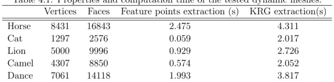
4.1 Properties and computation time of the tested dynamic meshes. . . . 63
4.2 Computation times for the tested dynamic meshes. . . 64
5.1 Retrieval performance of our method evaluated using five standard measures on the whole collection selected from SHREC 2012 data set and for each category. . . 80
5.2 (I) Screen shots of the null model (a) after different transformations: random noise (b), isometry (c), affine transformation (d), partiality (e), sampling (f), scale (g), topology (h). (II) Similarity results of the matching experiments. . . 82
5.3 Comparison of similarity estimation scores on the SHREC 2011 data set obtained by our method and the method proposed in [Barra 2013]. 83
5.4 Similarity estimation scores on the SHREC 2010 data set. . . 84
5.5 Retrieval performance for the McGill database. . . 86
5.6 Average execution times searching 3D models in McGill, SHREC 2010 and SHREC 2012 data sets. . . 88
6.1 Properties of the tested dynamic meshes.. . . 102
6.2 Evaluation of the mean square error of the motion compensation E(Π).104
6.3 Average execution times for Cow, Dance and Chicken models. . . 109
1 Chi-Square distribution table. . . 116
Chapter 1
Introduction
Contents
1.1 Field applications of 3D shapes . . . 7
1.2 Objectives and contributions . . . 9
1.3 Outline. . . 10
P
icture concept did not starts only with the advent of first computer, camera or scanner. The language of the image is reproduced since ancient times, with the beginning of this life. Where humans, in a long time ago, communicate among themselves via sign language and graphics. Up to now archaeologists are trying to decode their manuscripts to learn the secrets of the various people lives. But with the invention of the computer, the scanner or any image capture equipments, it has become necessary to look at ways to analyze and process this kind of digital data.1.1
Field applications of 3D shapes
In the last decade, the technological progress in telecommunication, hardware design and multimedia, allows access to an ever finer three-dimensional (3-D) modeling of the world. Nowadays, this kind of 3D contents is commonly used in several domain applications (see Fig.1.1) including digital entertainment and scien-tific simulation. The critical challenges with 3D models lie in their visualization, rendering, protection or transmission over channels with limited bandwidth and storage on media with low capacity.
In order to ensure interoperability exchanges and the interpretation of these par-ticular data, 3D objects must be represented according to standard formats. There exists many 3-D representations such as implicit surface, NURBS or voxel. But the most widely used representation of 3D shapes is the triangular surface mesh. This representation, consisting of vertices, edges and faces, is very widespread due to its simplicity. It contains geometrical information representing vertex coordinates in 3D space and topological information describing the incidence and adjacency relationship between vertices. In addition to its algebraic simplicity and high usability, 3D mesh representation is considered as an effective low-level model. Indeed, any kind of 3D models can be easily converted to 3D mesh representation.
8 Chapter 1. Introduction
Figure 1.1: The various fields of applications where 3D objects occupies an indis-pensable role.
While most researchers have focused on the field of 3D objects, now it is necessary to turn to 3D time domain (3D+t). 3D dynamic meshes are becoming a media of increasing importance. A 3D dynamic shape is usually represented by a se-quence of 3D meshes with constant connectivity and temporal information provided by time-varying geometry, only the vertex positions changes over time (see Fig. 1.2). Similar to pixel grid representation, this 3D content is subject to various processing operations such as indexation, segmentation or compression. However, surface mesh is an extrinsic shape representation. Therefore, it suffers from impor-tant variability under different sampling strategies and canonical shape-non-altering surface transformations, such as affine or isometric transformations. Consequently it needs an intrinsic structural descriptor before being processed by one of the aforementioned processing operations.
To meet these challenges, in this thesis, we focus to the intrinsic topological modeling based on Reeb graph and we intend to extend this principle for dynamic models.
- t
1.2. Objectives and contributions 9
1.2
Objectives and contributions
The research topic of this thesis work is the topological modeling based on Reeb graphs. Specifically, we focus on 3D shapes represented by triangulated surfaces. Our objective is to propose a new approach, of Reeb graph construction, which exploits the temporal information. The main contribution consists in defining a new continuous function based on the heat diffusion properties. The latter is com-puted from the discrete representation of the shape to obtain a topological structure. The restriction of the heat kernel to temporal domain makes the proposed function intrinsic and stable against transformation. Due to the presence of neigh-borhood information in the heat kernel, the proposed Reeb Graph construction approach can be extremely useful as local shape descriptor for non-rigid shape retrieval. It can also be introduced into a segmentation-based dynamic compression scheme in order to infer the functional parts of a 3D shape by decomposing it into parts of uniform motion. In this context, we apply the concept of Reeb graph in two widely used applications which are pattern recognition and compression. Application to pattern recognition
Reeb graph has been known as an interesting candidate for 3D shape intrin-sic structural representation. we propose a 3D non rigid shape recognition approach. The main contribution consists in defining a new scalar function to construct the Reeb graph. This function is computed based on the diffusion distance. For matching purpose, the constructed Reeb graph is segmented into Reeb charts, which are associated with a couple of geometrical signatures. The matching between two Reeb charts is performed based on the distances between their corresponding signatures. As a result, the global similarity is estimated based on the minimum distance between Reeb chart pairs.
Application to segmentation-based dynamic Compression
Skeletonisation and segmentation tasks are closely related. Mesh segmentation can be formulated as graph clustering. First we propose an implicit segmentation method which consists in partitioning mesh sequences, with constant connectivity, based on the Reeb graph construction method. Regions are separated according to the values of the proposed continuous function while adding a refinement step based on curvature and boundary information.
Intrinsic mesh surface segmentation has been studied in the field of com-puter vision, especially for compression and simplification purposes. Therefore we present a segmentation-based compression scheme for animated sequences of meshes with constant connectivity. The proposed method exploits the temporal coherence of the geometry component by using the heat diffusion properties
10 Chapter 1. Introduction
during the segmentation process. The motion of the resulting regions is accurately described by 3D affine transforms. These transforms are computed at the first frame to match the subsequent ones. In order to improve the performance of our coding scheme, the quantization of temporal prediction errors is optimized by using a bit allocation procedure. The objective aimed at is to control the compression rate while minimizing the reconstruction error.
1.3
Outline
The remainder of this manuscript is laid out as follows :
Chapter 2 presents a classification of different 3D object representations focusing on triangular 3D surface models. the fields and the area applications of 3D object are represented first. Then it reviews the different representations of three-dimensional objects regrouped in three main categories: surface models, volume models and linear models, specifically polygonal meshes while focusing on 3D shapes represented by surface meshes.
Chapter 3 introduces the different modeling 3D meshes specifying the bene-fits of using the topological modeling based on Reeb graphs. The final part defines the differential topology modeling by introducing the morse theory notion and giving a survey on Reeb Graph extraction methods.
Chapter 4 proposes a new Reeb graph construction approach which exploits the temporal information. The main contribution consists in defining a new scalar function. In this chapter, we introduce the heat diffusion principle, adapted to Riemannian manifolds, which is the core of the proposed scalar function. Then we describe our Reeb Graph construction method in detail. Finally we investigate the performance of our approach in terms of accuracy and robustness.
Chapter 5 presents a 3D non rigid shape recognition approach that uses the Reeb graph representation as local shape descriptor. We start by providing a brief overview of the most relevant work in the field of 3D pattern recognition. Then, we describe the proposed approach in detail. Finally, we evaluate the performance of our system by conducting a fair comparison with previous approaches from the state-of-the-art.
Chapter 6 proposes another application of Reeb graph representation in the context of dynamic mesh partitioning. First, we provide an overview of the various
1.3. Outline 11
existing work in the field of segmentation and compression of 3D mesh sequences. Second, we describe the proposed segmentation-based dynamic compression scheme. In order to examine the effectiveness of our compression system, we report the compression results and compare them to other 3D dynamic coding techniques from the state-of-the-art.
Finally, Chapter 7 concludes this manuscript. It provides a summary of contri-butions and presents directions of future work and open problems.
Chapter 2
3D shapes modeling
Contents
2.1 Introduction . . . 13
2.2 Field applications of 3D shapes . . . 13
2.3 Creation of 3D shapes . . . 14
2.4 3D shape modeling . . . 14
2.4.1 Linear Representations (Polygonal Meshes) . . . 14
2.4.2 Surface representations . . . 21 2.4.3 Volume representations . . . 24 2.4.4 Discrete models. . . 25 2.4.5 Fractal models . . . 25 2.4.6 Constructive models . . . 26 2.5 Conclusion . . . 26
2.1
Introduction
3D objets are commonly used in several domain applications, in this chapter we highlight the fields where 3D modeling is considered as an important issue. In addi-tion to the area applicaaddi-tions of these data, we are also interested to their hardware and software generation which is addressed in the second part of this chapter. After being created, 3D objects are modeled according to standard formats, in order to ensure their interoperability exchanges and their interpretation. In the last part of this chapter, we review the modeling of three-dimensional objects. We distinguish three main categories: surface models, volume models and linear models, specifi-cally polygonal meshes. We focus in this thesis on 3D shapes represented by surface meshes.
2.2
Field applications of 3D shapes
The recent technological progresses in the fields of telecommunication, com-puter graphics and multimedia allow access to an ever finer three Dimensional modeling of the world. 3D shape modeling occupies a very important place in the computer graphics world. It is used in areas as diverse as medicine, video
14 Chapter 2. 3D shapes modeling
games, computer-aided design... It is very interesting to 3D objects whenever we want to make virtual tours of museums or to model real and/or virtual 3D scenes. Today with the technological advances in the medical field, 3D objects are integrated in computer-aided diagnosis through CT (Computerized Tomography) and MRI (Magnetic Resonance Imaging) scans. Furthermore, they are used in computer-assisted surgeries. Furthermore, it is worth mentioning that 3D objects play an unavoidable role in geographic information systems such as astronomy, geology, and mapping.
Obviously, we cannot evoke all of the application areas. However, it is im-portant to cite the studies and simulations of physical phenomena around us. This area is based on the numerical simulation by using finite element analysis methods and by solving differential equations. By this way, it is possible to study the propagation of electromagnetic waves through the human body, and consequently evaluate their dangerousness.
In what follows, before we turn to the modeling of 3D objects, we briefly back on methods of creating the underlying 3D models.
2.3
Creation of 3D shapes
There are specialized 3D CAD (Computer-Aided Design) software (AutoCAD, Autodesk Maya, Autodesk 3ds autodesk inventor ...) and geometric modelers that are generally used to obtain a geometric and topological representation of virtual 3D object or scene.
The representation of a real 3D object can be obtained by using special hardware devices called range scanners. The scanning devices can produce data (range images or point clouds) which is very dense without necessarily reflecting the curvature of the object. Indeed, these devices produce a highly redundancy data, especially on smooth areas of the mesh, which is difficult to process. To alleviate this problem it is possible to reduce the redundancy through simplification methods. After the data acquisition phase, several modeling types can be used to rep-resent these 3D-data in order to ensure their interoperability exchanges and interpretation. Among these 3D modeling types, we can cite: surface representa-tion, volume representarepresenta-tion, and linear representation.
2.4
3D shape modeling
2.4.1 Linear Representations (Polygonal Meshes)
Linear models are widely used thank’s to their simplicity. They are characterized by a very understood modeling ability, which allows them to represent any complex
2.4. 3D shape modeling 15
topology object. Among the linear representation, we distinguish polygonal meshes, which are represented by a set of vertices connected by edges forming facets. The most commonly used geometric forms to represent these facets are triangles (3-D triangular meshes) that will be used in the context of our studies. 3D meshes belong into the surface modeling class that provides roughly a representation of an object, which is very complex and adapted to the shape design. This kind of representation is defined by a geometric information represented by the vertex coordinates in 3D space and topological information describing the incidence and adjacency relation-ships between vertices, edges and faces. The topological information includes the degree of a face which means the number of edges which it compose (in the case of triangular mesh, the degree of faces is equal to 3) and the vertex valence, which is the number of its incident edges. These two pieces of information are explained in Fig. 2.1.
Figure 2.1: Triangular mesh illustrating the topological information.
2.4.1.1 Topological properties of 3D surfaces
The key concept when studying the topological properties of surfaces, is the notion of homeomorphic topological spaces. Properties of figures unchanged by homeomorphisms are called topological properties, or topological invariants. Homeomorphism: Two 3D topological surfaces S and S′ are homeomor-phic only if there is a continuous bijection φ between the two surfaces φ: S → S′ such as the inverse function φ−1 is also continuous. Intuitively, S and S′ are called homeomorphic if the surface S can be stretched and bent without breaking to fit the shape of S′. The notion of homeomorphism allows defining equivalence classes in the surface spaces. In particular, it allows introducing the varieties, defined as follows: A triangle mesh can be 2-manifold if it satisfies the following properties:
• Property local disk: if there is on each point of the surface a neighborhood homeomorphic to an open disk or an open semi-disk.
• Property scheduling edges: the adjacent edges of each vertex must be arranged in a circular fashion.
• Neighborhood Property face: each edge of the mesh must have exactly two adjacent faces if it is an inside edge to the mesh and only one face if it is an
16 Chapter 2. 3D shapes modeling
boundary edge.
To test whether a mesh is a manifold or not, it is important to introduce the concepts of regular vertex and regular edge.
• Regular vertex: all its neighbors can be rearranged to define a unique path. • Regular edge: it is shared by a maximum of two triangles.
According to the aforementioned definitions, we can demonstrate the following property: a triangular mesh is manifold only if all its vertices and edges are regular. A mesh is called non-manifold if it has at least one edge connected with at least three sides, so it will be impossible to differentiate the inside and the outside without ambiguity.
Neighborhood regularity, depends on the valence of the vertices, is also a very important property for triangular meshes. It depends on the valence of the vertices, As illustrated in Fig.2.2, we distinguish three mesh structures:
• Irregular mesh: all vertices have different valence values due to the the lack of consistency in how to connect the vertices
• Regular mesh: all vertices have the same valence.
• Semi-regular mesh: a small number of vertices are irregular and the remains have the same valence.
Figure 2.2: From left to right: an irregular mesh, semi-regular mesh and regular mesh.
It is also possible to distinguish other types of meshes such as:
• Conform mesh: it has all geometric elements of non zero areas and the inter-section of two geometric elements of the mesh is either empty or reduced to a vertex or an entire edge. Connecting the middle of a ridge and a summit will, for example prohibited.
2.4. 3D shape modeling 17
• Multi-resolution mesh: it offers several levels of information and good support for progressive rendering, scalable compression, and data transmission. The aim is to represent the surface at different levels of detail. The decomposition process of the original mesh into intermediate meshes is reversible. From the coarser mesh it is possible to reconstruct all levels of approximations until reaching the fine one (coarse to fine). Or, conversely, simplifying a fine mesh to obtain a coarser approximation (fine to coarse). Fig. 2.3(a) and (b) show the simplification and the reconstruction stages. It is important to note that the hierarchical decomposition techniques depend on the mesh connectivity constraints, while the simplification approaches are applicable on any mesh connectivity. → → → ... → (a) → → → ... → (b) Figure 2.3:
Some triangular meshes respect the Delaunay criterion. In this case, the circumscribed circles of triangles forming the mesh are do not contain any vertex. Euler′s characteristic: Let M be a manifold mesh, oriented and without board, composed of F triangles, E edges and V vertices. Let G be the genus of the mesh M , which corresponds to the maximum number of closed curves without common points that can be drawn inside this surface without disconnecting it. The Euler’s formula [Coxeter 1989]is given by:
χ = V − E + F. (2.1)
This Euler’s characteristic χ is related to the genus G of the surface. Indeed, the genus is a global topological feature that allows to determine equivalence classes in the varieties of space. It reflects more or less its topological complexity and is intuitively equal to the number of handles in the shape (see Fig.2.4). More specifically, the genus G of a 3-D object can be expressed by the following equation:
G = 2c− b − χ
2 , (2.2)
where c is the number of connected components and b is the number of edges of the surface. In practice, a small number of meshes satisfies the regularity property.
18 Chapter 2. 3D shapes modeling
(a) (b) (c)
Figure 2.4: A sphere (a) is of genus 0, a torus (b) is of genus 1 and a 2-torus is of genus 2.
However, under certain assumptions, we can demonstrate that the average valence of the vertices is 6. This result is a direct consequence of the Euler’s characteristic. The orientation of a face is defined according to the cyclic order of vertices and the right-hand rule. There are two possibilities: the orientations of two adjacent faces are compatible if there exist two vertices shared across commands in both sides. So the complete mesh is called orientable if we can find a combination of orientations in all sides such that each pair of adjacent faces in the mesh is compatible.
2.4.1.2 Standard formats of representation
Various standard formats use the naive representation of polygonal meshes. Most of these file formats are represented in an ASCII form such as the Virtual Reality Modeling Language (VRML), the 3D Object File Format OFF, the Wavefront OB-Ject format OBJ, the Stanford University PoLYgon format PLY, ... . The storage strategies of these file formats are very similar. The geometry is generally repre-sented by an indexed list of vertex coordinates and the connectivity is composed of a list of faces, where each face is represented by the indices of its vertices. The global file consists of the geometrical information followed by the topological one as shown in Fig.2.5The principle is to encode the mesh geometry by using a matrix G
2.4. 3D shape modeling 19
with V rows and 3 columns, with V being the number of vertices:
G = Xx 1 X y 1 X1z X2x X2y X2z X3x X3y X3z . . . . . . . . . XVx XVy XVz (2.3) where Xx l, X y
l and Xlz are the cartesian coordinates of the vertex indexed by l in the surface mesh M . The mesh connectivity is also represented by a matrix denoted by Γ of size F × 3 (where F is the number of faces).
Γ = v11 v12 v13 v12 v22 v23 v13 v32 v33 . . . . . . . . . vV1 v2V v3V (2.4)
where v1i, vi2 and vi3 are the integer indices of three vertices forming the ith triangle of M .
2.4.1.3 From 3D to 3D+t domain
Technological progress in the field of multimedia and computer vision has led to the exploitation of the time factor t to process 3D objects. While the majority of research in this area was based on 3D objects, now, it is necessary to turn to 3D time domain (3D+t). Indeed, dynamic3D shapes are becoming a media of increas-ing importance used mainly in the field of video games, movies, computer-aided design, and medical imaging. This kind of data is usually represented by key-frame sequences of 3D triangular meshes sharing the same connectivity and temporal information provided by time-varying geometry. Only the vertices position changes over time. As for static models, dynamic models can be formalized mathematically as follows: Let’s designate by (Mt)t∈{1,...,T } a sequence of 3D meshes (where T is the number of frames). Under the hypothesis of a fixed connectivity, by considering Γ (given by eq. 5.3), the mesh geometry at time t is represented by a matrix Gtof dimension 3× V (where V is the number of vertices) defined by:
20 Chapter 2. 3D shapes modeling Gt= X1,xt X1,yt X1,zt X2,xt X2,yt X2,zt X3,xt X3,yt X3,zt . . . . . . . . . XV,xt XV,yt XV,zt (2.5)
where Xl,xt , Xl,yt and Xl,zt are the cartesian coordinates of the vertex indexed by l at time t Mt. Fig.2.6 shows some key-frame sequences of 3D triangular meshes. Animate a 3D object consists to describe the motion and/or the deformation that it
Figure 2.6: Some examples of dynamic 3D meshes.
undergoes during a specified time period. Most often this amount of data, needed to generate a dynamic 3D object represented by key-frame sequences, describes the time evolution of a 3D surface (i.e change of the vertex positions, normals, colors ...). The first approach that has been adopted to generate animated content specifies the properties of the 3D object as a function of time. Obviously, such approach (heavy and non-intuitive) is not usable in practice, even in the case of simple 3D models. To simplify the task of animated content generation, the majority of animation techniques proposed to describe the animation operator according to the motion patterns and / or deformation.
In general, the creators of 3D animated objects can be classified into two main categories: animation using descriptive models and procedural animation.
2.4. 3D shape modeling 21
The first category is based on an explicit representation of the animation that describes, for each key frame, the motion field parameters or associated deforma-tion. This type of animated 3D objects creation allows designers to accurately control the progress of the animation. However, it requires a significant volume of user interaction for the specification of key-frames. On the other hand, the second category is primarily based on a set of physical, mathematical or behavioral laws. It generates dynamically and automatically realistic animations and high quality while taking into account the interaction with user or changes in the environment. The disadvantage is that the control of the time flow of the animation is limited. To store these animated models, there are various standards of representation formats such as:
• The standard VRML Virtual Reality Modeling Language (WRL file exten-sions), developed by the Web3D Consortium is a description language for interactive 3D virtual universe. It represents a 3D scene as a hierarchical tree whose nodes describe objects or scene properties (3D meshes, basic shapes, sounds, light sources, colors ...).
• The standard X3D eXtensible 3D extends the VRML standard by introducing new features and a description format. This representation allows to describe the animated humanoid, physical interactions between solids, and particle systems necessary for modeling elements such as fire, smoke, snow ...
• The H-Anim standard is another description language for character anima-tions articulated human model. H-Anim representation allows modeling the anatomical skeleton of a 3D articulated character by a hierarchical tree struc-ture.
2.4.2 Surface representations
Surface models are composed of k-simplices which may be the vertices (0-simplex), the edges (1-simplex) or triangles (2-simplices). The polygonal mesh belongs to this type of modeling, the object is represented by several polygonal elements and the surface will be built by assembling its elements. This representation model is classified into three types of surfaces: parametric, implicit, and subdivision surfaces. 2.4.2.1 Parametric surfaces
The parametric representation is characterized by the definition of each surface point by a equation with two parameters η and µ represents the application of a region of the plane (η, µ) in three dimensional space. Fig. 2.7 shown an example of a parametric surface. S(η, µ) = ffx(η, µ)y(η, µ) fz(η, µ)
22 Chapter 2. 3D shapes modeling
It is preferable that the functions fx, fy and fz are polynomial functions to obtain an accurate approximation of the surface and a simple geometric interpretation of their coefficients. This type of surfaces is obviously used to interpolate or approach a set of points. These points are usually organized in a matrix form. These
para-Figure 2.7: A parametric surface example.
metric models include a large family of surfaces. We can distinguish primarily the sub family of curves and Bezier surfaces (area B-Splines / NURBS) that are char-acterized by a set of points called control points forming a grid. The disadvantage lies in the movement of a control point which affects the entire object.
2.4.2.2 Implicit surfaces
Contrary to parametric models that explain the point coordinates, the im-plicit formalism id defined defined according to a particular mathematical form [Bloomenthal 1997]. It consists at representing a surface as a set of points in space checking a property which is generally related to the value taken at these points. An implicit surface S is defined as the set of zeros of a function f in R3 in
R. The set of points P = (x, y, z) of the implicit surface S defined by f is one that satisfies the following equation:
f (x, y, z) = 0. (2.6)
From this formulation and using the sign of the function we can directly concluded the information about the relationship between all points in three-dimensional space:
• if f(x, y, z) < 0; p will be on the outside of the object to be modeled. • if f(x, y, z) > 0; p will be inside the object to be modeled.
• if f(x, y, z) = 0; p will be on the surface of the object to be modeled.
The advantage is to separate the space into two components: inside and outside the area. So one can easily determine the position of a point relative to the boundary
2.4. 3D shape modeling 23
Figure 2.8: Example of an implicit surface.
surface. This representation model can be considered as the surface model or volume model because otherwise described the volume defined by the surface. This type of representation allows modeling of rounded shapes. It is best suited for medical imaging, physical processes [Terzopoulos 1987], human modeling and modeling smooth objects [Turk 1999].
Implicit surfaces are divided into two categories: algebraic surface that is mathematically defined as the set of roots of a polynomial function more or less degree of complex (2, 3or4). Non algebraic surface that serves to model an object by a set of particles. Fig. 2.8shows an example of implicit algebraic surface defined by the equation: x4− 5x2+ y4− 5y2+ z4+ 5z2+ 11.8 = 0.
2.4.2.3 Subdivision surfaces
A subdivision surface [D. Zorin 2000] is a smooth surface defined as the limit of a sequence of refinements, applied to a control mesh. Fig.2.9describes the hierarchical aspect of the subdivision. These refinements include modifying connectivity and
Figure 2.9: Illustration of the hierarchical aspect of the subdivision.
geometry by adding, moving vertices to obtain a mesh that tends toward a smooth boundary.
In general, a subdivision scheme is described by:
• A topological component: all subdivision schemes are changing the initial mesh connectivity, then we can distinguish two types of schemes: primal patterns that retain the old highs, and dual patterns that suppress.
24 Chapter 2. 3D shapes modeling
• A geometric component: the vertices position change can be interpreted as a smoothing of the original mesh. One can also distinguish two types of schemes: the interpolating patterns that keep the position of initial vertices and non-interpolating schemes that change their positions by moving them.
We distinguish several subdivision schemes differentiated according to the type of polygons treated and the type of operation performed subdivision. We quote as well the nature of schemes approximating where the control points are not located on the boundary surface. It is difficult to estimate the resulting surface. Meanwhile, we find the nature of interpolating subdivision schemes in which all control points lie on the boundary surface, since the movement includes only the newly inserted vertices.
2.4.3 Volume representations
3D volume representations are particularly suited for medical imaging (3D Volume Representation of tumor through the use of Magnetic Resonant Imaging) ref(3D Volume Representation of brain tumor using image processing). 3D volumetric medical images are usually analyzed as a sequence of 2D image slices [Shen 2008] due to concerns over the exponential increase in computational cost in 3D. These kind of representations allow structural modeling objects by one or serval primitives of volume nature, generally ordered in graph form. There are different types of primitives such as cylinders, superquadrics the hyperquadrics and other implicit polynomial. Thus we can classify these models into two groups:
• Quantitative models having a great modeling power. • Qualitative models for symbolic modeling.
2.4.3.1 Superquadrics
The superquadric model is an extension of quadric, this primitive has the capability to admit an implicit and a parametric forms, the most commonly used are the super-ellipsoid. The high description capability is one of the advantages of this model despite the small number of parameters. These models are well suited to the field of medical imaging. They provide an efficient modeling, in both space and time, of certain organs such as the heart.
2.4.3.2 Hyperquadrics
The hyperquadric model is a general case of superquadric, but it only makes an im-plicit representation compared to superquadric model. It differs from superquadric model by the non symmetry of its representation and its descriptive power. De-spite the high description power of hyperquadric model, its use remains marginal compared to that of superquadric. As a result, the complexity and the lack of para-metric formulations of hyperquadric primitives make them less reliable. Similarly to
2.4. 3D shape modeling 25
superquadrics, these primitives are used mainly for the reconstruction and modeling of 3D objects in the medical field.
Table 2.1: A Comparison between 3D shape modeling techniques.
Model advantages disadvantages
3D Mesh
algebraic simplicity lack of continuity high usability scale dependence arbitrary topology
Parametric surfaces
high continuity no arbitrary topology mathematically defined complex handling compactness
local control
Implicit surfaces
compactness complex handling
descriptive ability limited to organic forms
complexity sampling
Subdivision surfaces
high continuity no defined mathematically arbitrary topology
algebraic simplicity compactness multiresolution local control
Volume Representations compactness limited descriptive ability Discrete Model high usability scale dependence
size memory
fractal Model descriptive ability restricted
to natural objects
Constructive Model complex rendering
2.4.4 Discrete models
By using a discrete model, an object is represented by the set of spatial cells occupied by the volume of the object in space. This representation is obtained using a three-dimensional array consisting of fixed-size cubes called voxels. The discrete models are very simple however, they are very expensive in terms of memory, and they are often used in the medical field.
2.4.5 Fractal models
The objective is to represent a curve or an irregular shaped surface by an iterative method. This kind of representation was used for 2D image compression and has
26 Chapter 2. 3D shapes modeling
been extended to 3D object compression. It is used only to represent natural objects such as mountains and clouds... It can represent repeated patterns many times. These are usually recursive functions using an initial pattern and a replacement pattern. For surfaces, the objective is to divide each segment in half, from an initial triangle, and change the height of the midpoint of each segment randomly
2.4.6 Constructive models
These models are widely used in computer-aided design (CAD) applications. They represent an object by a tree called build tree whose leaves are the objects and the non-terminal nodes are considered as operators.
2.5
Conclusion
Table 5.1 summarizes the main advantages and drawbacks of each model repre-sentation categories described in this chapter. For a larger survey of 3D surface representations, the interested reader should refer to additional reference on polyg-onal meshes and their applications in geometry processing [Botsch 2007]. In the context of our work, we focus on the 3D triangular surface meshes, which have a fairly wide descriptive power allows them to manipulate in a simple way the objects of arbitrary topology. However this representation is extrinsic, it suffers from high sensibility against affine and isometric transformations. Therefore to overcome this problem it seems necessary to look for defining computational intrinsic modeling which will be addressed in the next chapter.
Chapter 3
Background knowledge on 3D
shape intrinsic modeling
Contents
3.1 Introduction . . . 27
3.2 Geometry modeling . . . 27
3.2.1 Spectral and Laplacian based modeling . . . 28
3.2.2 Conformal geometry based modeling . . . 32
3.2.3 Riemannian geometry based modeling . . . 35
3.3 Topology modeling . . . 38
3.3.1 Curve skeletons . . . 38
3.3.2 Segmentation . . . 41
3.3.3 Differential topology based modeling (Reeb Graph). . . 44
3.4 Conclusion . . . 47
3.1
Introduction
In the previous chapter, we mentioned that the 3D triangular meshes are frequently used to represent 3D objects, thanks to their algebraic simplicity and high usabil-ity. However, their only downside lies in the fact that a 3D triangular mesh is an extrinsic modeling, and any applied topological, affine or isometric transformation may affect this representation. For this reason, we need to go through an intrinsic modeling before processing this kind of 3D data. In this chapter, we review the intrinsic modeling of three-dimensional objects. In particular we distinguish two categories: geometry and topology based modeling. For each category, we describe three representative classes of approaches. Finally, we give some theoretical prelim-inaries and existing work about Reeb graph based modeling which is the core of our research.
3.2
Geometry modeling
The surface geometry is often referred to as its shape. It is primarily defined by the set of its intrinsic characteristics varying under smooth transformations. In the
28 Chapter 3. Background knowledge on 3D shape intrinsic modeling
following, we present three classes of geometry based modeling methods for surface mesh intrinsic description.
3.2.1 Spectral and Laplacian based modeling
Before beginning this section, let us answer the question: what defines spectral modeling? If we suppose a closed system of basic equations and introduce into this system a finite expansion of dependent variables by means of functions such as Fourier. Thus we obtain, for these function coefficients, series of coupled non linear differential equations, due to the orthogonality properties of the used spatial functions. By using the Fourier transform, the horizontal spatial dependence is removed. These function coefficients depend only on the time and the vertical coordinate. To solve the coupled non linear differential equa-tions, a simple time-differencing and a vertical finite differencing are mostly applied. Spectral modeling can be considered as spectral modeling synthesis, noted SMS, which is an acoustic modeling technique adapted to any signals including speech. It allows to replace the portions of the time-domain signal by their short-time Fourier transforms. This principle ensures that the sound representation is very similar to the perception of sound by the brain. This allows to reduce the calculation complexity based on perceptual modeling, and more fundamental data structures perception. Thank’s to the short-time Fourier transforms, the famous MP3 audio compression format can reach an order of magnitude information reduction with little or no loss. That is also due to the fact that it prioritizes the conserved data in each spectral frame based on psychoacoustic principles.
In the case of manifolds, various existing work used the spectral transform by putting the given surface into one-to-one correspondence with a simpler do-main [Zhou 2004], or to segment the surface into a set of simpler domains [Lee 1998,Pauly 2001]. Therefore, it is possible to define a frequency space in these simpler domains. Authors in [Sokrine 2005] proposed calculating geometry aware basis functions, defined as solutions of some least-squares problems.
3.2.1.1 Spectral mesh processing
Spectral mesh processing implies the use of eigenvalues, eigenvectors, or eigenspace projections from suitably defined mesh operators to perform appropriate tasks. The basic idea consists in constructing a matrix, based on the topological and/or geometrical information of the input mesh. This matrix representing a discrete linear operator can be considered as an incorporating pairwise incidence or adjacency relationships between vertices, edges and faces in the mesh. Once the matrix is constructed, an eigen-decomposition is then performed by computing the set of it eigenvalues and eigenvectors. Based on the resulting structures from the decomposition, which is used in a problem specific manner, the solution is obtained.
3.2. Geometry modeling 29
The primary motivation for proposing spectral mesh processing approaches is the pursuit of Fourier analysis in the manifold setting. Methods applied in the spectral domain, project the signal in a transformed space. They propose concepts specially adapted to the underlying irregular three-dimensional meshes. The objective is to infer intrinsic geometrical surface characteristics by computing its spectral transform.
Fourier analysis
In order to define the concept of the Fourier transform, we begin by intro-ducing the case of a closed curve in the continuous setting. Supposing a square integrable periodic function notes f : x∈ [0, 1] 7→ f(x), with f a function defined on a closed curve parameterized by normalized arc-length [Levy 2006]. This function, f , is decomposed into an infinite series of sinus and cosine of increasing frequencies:
f (x) = ∞ ∑ k=0 ¯ fkHk(x); H0 = 1 H2k+1 = cos(2kπx) H2k+2 = sin(2kπx) (3.1)
being ¯fk the decomposition coefficients calculated according to equation4.4, the set of these coefficients are called the Fourier Transform (FT) coefficients of the function f . ¯ fk=< f, Hk>= ∫ 1 0 f (x)Hk(x)dx, (3.2)
where < ., . > denotes the inner product (i.e. the dot product for functions defined on in interval of [0, 1]).
The study of a periodic function by Fourier series has two components: analysis and synthesis. During the analysis, the Fourier coefficients are determined. The synthesis allows to reconstruct the function f using the resulting coefficients ¯fk by applying the inverse Fourier Transform F T−1.
Now let’s generalizing these notions to arbitrary manifolds. We suppose the function Hk of the Fourier basis is the eigenfunctions of ∂2/∂x2:
−∂2H2k+1(x)
∂x2 = (2kπ)
2cos(2kπx) = (2kπ)2H2k+1(x). (3.3)
The eigenfunctions H2k+1 are associated with the eigenvalues (2kπ)2. To under-stand the geometric significance of the eigenfunction, in the next section, we study the discrete setting by considering the eigenfunctions as orthogonal non- distorting 1D parametrization of the shape. In the next sections, we focus on the Laplacian operator in the discrete and continuous settings and present its utility for 3D shape modeling.
30 Chapter 3. Background knowledge on 3D shape intrinsic modeling
Among the early work in this field, we cited the original method proposed by Taubin [Taubin 1995b]. He demonstrated that the signal processing formalism could be applied correctly to geometry processing. The similarity between the eigenvectors of the graph Laplacian and the basis functions used in the discrete Fourier transform is the base of the proposed method in [Taubin 1995b]. The used Fourier function basis allows decomposing a given signal into a sum of sine waves of increasing frequencies.
Figure 3.1: The Fielder vector gives a natural ordering of the nodes of a graph. The displayed contours show that it naturally follows the shape of the dragon.
Authors in [Isenburg 2009] have employed the spectral graph theory to calcu-late an ordering of mesh vertices in order to simplify the processing. Fig. 3.1
shows what it looks like for a snake-like mesh (it naturally follows the shape of the mesh)[Levy 2006]. The Graph Laplacian denoted L = (ai,j) is a matrix defined as follow:
ai,j = wi,j > 0 if (i, j) is an edge
ai,i = −
∑ jwi,j
ai,j = 0 otherwise
(3.4)
being wi,j the weights associated with the graph edges. The interested reader should refer to [Lévy 2009] for more details and explanations.
Laplacian Beltrami : continuous setting
In the continuous setting, the laplacian operator called also laplace operator is extremely important in mechanics, electromagnetic, wave theory, and quantum mechanics. The laplacian operator is defined as the divergence of the gradient given by the following expression :
∆ = divgrad =∇.∇ =∑ i ∂2 ∂x2 i . (3.5)
It is important to note that the eigenfunctions of the Laplace Beltrami (Manifold harmonics) define basic functions. However, the problem occurs in the calculation
3.2. Geometry modeling 31
of eigenvectors for large mesh size. Considering discrete meshes, many cotangent schemes have been proposed to estimate the Laplace-Beltrami operator [Meyer 2002, Reuter 2006,BelkiIn 2008] in order to overcomes the current limits.
3.2.1.2 Applications
Spectral modeling in the case of 3D shape, consists in computing the eigenvalues and eigenvectors of a discrete laplace operator. This eigen-decomposition is applied in various applications to achieve different tasks. Furthermore, a signal defined on a triangle mesh can be projected into the eigenvectors taken as a basis. The obtained coefficients of spectral transform can be analyzed or processed further. In this paragraph we present the applications which used the spectral transform or the eigenvectors of mesh Laplace. This king of modeling occupies a very important position in various fields. Among these, Karni and Gaustman’s work [Karni 2000] which consists in realizing a 3D shape compression scheme based on a spectral decomposition method. The main idea is to project the mesh geometry on the eigenvectors of the Laplacian matrix associated to the object. Thus, a spectrum (see Fig. 3.2) represented by geometrical coefficients (spectral coefficients) is then quantized and transmitted in ascending order of the frequency associated with each coefficient. This spectral analysis is considered as a generalization of the cosine transform on irregular surface meshes.
Figure 3.2: Geometric spectrum of simplified Bunny mesh (100 vertices).
In the literature, there are several watermarking techniques applied in the spectral domain to improve the robustness and imperceptibility tasks. To obtain a frequency representation of the mesh, they use the Laplacian matrix of size D (N × N). The obtained N eigenvalues and N eigenvectors are standardized and sorted in ascending order according to their associated frequencies. The N spectral components are calculated respectively by projecting the cartesian coordinates (x, y, z) on the normalized and stored eigenvectors. Liu et al. [Lui 2013] have used the classical spectral analysis to insert the watermark into 3D meshes. Their method consists in devising the low frequency part of the spectrum in 5 mesh patches. A bit is then inserted in each patch by changing the relative relationship between a certain selected spectral amplitude and the average of the different


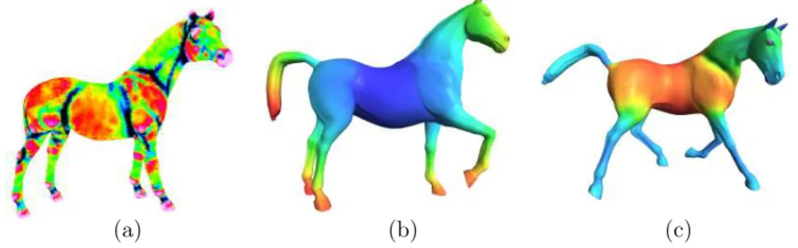


![Figure 4.5: Visual comparison between Lavoué et al. [Benhabiles 2012] algorithm (b), Tierny et al](https://thumb-eu.123doks.com/thumbv2/123doknet/7708741.246939/73.892.213.640.411.1010/figure-visual-comparison-lavoué-et-benhabiles-algorithm-tierny.webp)