HAL Id: hal-01847811
https://hal.archives-ouvertes.fr/hal-01847811
Submitted on 7 Dec 2018HAL is a multi-disciplinary open access archive for the deposit and dissemination of sci-entific research documents, whether they are pub-lished or not. The documents may come from teaching and research institutions in France or abroad, or from public or private research centers.
L’archive ouverte pluridisciplinaire HAL, est destinée au dépôt et à la diffusion de documents scientifiques de niveau recherche, publiés ou non, émanant des établissements d’enseignement et de recherche français ou étrangers, des laboratoires publics ou privés.
Near infrared thermography with silicon FPA
-Comparison to MWIR and LWIR thermography
Yann Rotrou, Thierry Sentenac, Yannick Le Maoult, Pierre Magnan, Jean
Farre
To cite this version:
Yann Rotrou, Thierry Sentenac, Yannick Le Maoult, Pierre Magnan, Jean Farre. Near infrared ther-mography with silicon FPA -Comparison to MWIR and LWIR therther-mography. Quantitative InfraRed Thermography Journal, Taylor and Francis, 2006, 3 (1), pp.93-115. �10.3166/qirt.3.93-115�. �hal-01847811�
Near infrared thermography with silicon
FPA - Comparison to MWIR and LWIR
thermography
*Yann Rotrou* — Thierry Sentenac* — Yannick Le Maoult* —
Pierre Magnan** — Jean Farré**
*Centre de Recherche sur les Outillages, les Matériaux et les Procédés (CROMeP) Ecole des Mines d’Albi, route de Teillet, 81000 Albi, France
{rotrou, sentenac, lemaoult}@enstimac.fr
**Laboratoire de Conception d’Imageurs Matriciels Intégrés (CIMI) SUPAERO, 10, avenue Edouard Belin, 31055 Toulouse, France {magnan, jfarre}@supaero.fr
ABSTRACT: An ideal thermographic camera could be defined as an uncooled system with high
spatial and thermal resolutions featuring a video frame rate, and a short calibration process. In this paper a measurement system based on Silicon FPA operating in the Near Infrared spectral band (0.7 − 1.1 µm) is proposed. This system offers an excellent spatial resolution, a low cost and compactness. With a specific radiometric model, this system can accurately measure temperatures, in a broad temperature range, from 400 up to 1000°C. A comparison with two commercial infrared cameras is performed between 400 and 700°C.
1. Introduction
For various technological reasons, the first infrared thermographic systems to be developed were scanning cameras. They came equipped with a cooled high cutoff wavelength materials (InSb or HgCdTe) mono detector, typically operated at liquid nitrogen temperature. Such systems present good thermal sensitivity characteristics, and are often still considered as the reference of thermography in military and laboratory applications. Latter infrared measurement systems were developed with InSb, PtSi and HgCdTe detectors arrays. Such infrared systems do offer better spatial resolution, but suffer from spatial response non uniformities. Due to cooling requirement, these systems remain relatively costly. Applications call for development of larger arrays and of detectors operating at ambient temperatures or so. Recently, new uncooled microbolometer cameras, designed especially for industrial process control (surveillance, predictive maintenance, automotive…), presenting good uniformity characteristics at lower costs, have emerged. In this context, video FPA with silicon detectors seem to offer interesting prospects, and can be used to obtain good temperature measurement. They operate at ambient temperature, are relatively cheap, light weight, compact, and do offer high spatial resolution. In some industrial applications, temperature measurements have already been demonstrated with such cameras, above 800°C. (Meriaudeau et al., 2003).
The purpose of this paper is to show that accurate temperature measurements from 400 to 700°C (end even 1000°C) can be achieved with silicon FPA cameras, thanks to a specific radiometric model, and a very short calibration process. Then a comparison with traditional thermographic cameras is provided.
The first part deals with the radiometric modeling using only one set of parameters for all integration times. Starting from the classical model used for IR scanning cameras, the influence of operating in the NIR spectral range is presented. Some necessary corrections to be efficient at low temperatures are included, and finally a specific radiometric model is established.
In the second part, a very short radiometric calibration procedures is proposed and compared to the ones used classically. Accurate results over broad temperature range have been obtained. Few points of calibration are needed and the parameters are identified without initialization.
In the third part, a comparison of the performances between silicon FPA1
operating in the NIR and two well-known commercial infrared scanning cameras2,
operating in the MWIR and LWIR, is realized. Intrinsic parameters (accuracy, fidelity, NETD, sensitivity) are presented. Finally true temperature measurement is introduced and sensitivity to the emissivity of the observed material is also discussed.
1 The CCD silicon FPA is the Prosilica EC1380. The CMOS silicon FPA studied in section
2.4 is the Prosilica CV1280.
2. Radiometric modeling
The radiometric model of a detector describes the relation between the incident flux Ф and the output signal Id. The apparent temperature T - the temperature of a
blackbody emitting the same incident flux Ф - is used.
First, one of the “traditional” radiometric models designed for infrared cameras is reminded. It is valid for a single detector with a linear photo response. Then we explain why this model is not totally suited to silicon FPA in the 300 - 1000°C temperature range, and we propose a specific radiometric model. Last, we detail the corrections, required necessary to obtain performances comparable with IR cameras.
2.1. Traditional infrared radiometric model
Let us consider an IR camera observing a black body at temperature T. The system is composed of a filter and a classical objective - their spectral transmittances are noted
τ
f(λ
)and respectivelyτ
o(λ
) -, and a detector with spectral quantumefficiency
η
e(λ
). We denoteτ
a(λ
) the spectral transmittance of the atmosphere.Then the output signal of a single detector with a linear photo-response is:
∫
=Kti
τ
λ
τ
λ
τ
λ
η
λ
Lλ
T dλ
T
Id0( ) . . a( ). f( ). o( ). e( ). 0( , ). [1]
with ti the integration time, and where:
1 ) . exp( . ) , ( 2 4 3 0 − = − T C C T L
λ
λ
λ
[2]is the Planck’s law expressed in photons/(s.m2.sr.µm), where C2 and C3 are the second and the third radiation constants (C2 = h.c/k and C3 = 2.c). h is the Planck’s constant (h = 6.62 10-34 J.s), c is the speed of light (c = 2.99 108 m/s) and k is the Boltzmann’s constant (k = 1.38 10−23 J/K). The spectral support of η(λ)
e ,
characteristic of the detector (0.4 -1.1 µm, 3 - 5µm or 8 – 12 µm) is finite, and as a result the range of integration is also finite and. Lastly, to simplify, we note:
) ( ). ( ). ( ). ( ) (
λ
τ
aλ
τ
fλ
τ
oλ
η
eλ
W ≡ [3]Next, the introduction of an effective wavelength
λ
e allows to establish a modelwithout preliminary knowledge of the function W(λ), and avoids the difficulty of extracting T from equation [1], by writing I0(T)
) , ( ). ( . . ) ( 0 2 0T K tiW L T Id =
λ
eλ
e [4] 1 ) ) ( exp( ). ( ) ( 0 − = T B ti A T I e e dλ
λ
[5] with 4 3 2. ( ). . ) ( e =K W e C −e Aλ
λ
λ
and e e C Bλ
λ
) 2 ( = .It is known (Kostkowsky et al., 1962) that strictly speaking, the effective wavelength depends on the black body temperature. A constant C is introduced to take into account this variation:
1 ) exp( . . ) ( 0 − = TB C ti A T Id [6]
This equation describes the ”classical” model with three parameters (A, B, C).
2.2. Our approach
For MWIR and LWIR scanning cameras, this radiometric model [6] is applied with a single integration time ti , and a constant effective wavelength λe. The set of
parameters (A, B, C) deals with one configuration of the camera. Typically, the temperature range from 300 to 700°C can be covered with two or three different aperture values, and so the camera is calibrated with 2 or 3 sets of parameters (A, B,
C). The same approach can be used with silicon FPA, where measurement over very
small temperature ranges above 300°C (Sentenac et al., 2002) or over small temperature range above 800°C (Meriaudeau et al., 2003) are realized with few integration times, associated with the same number of parameters sets.
Here we want to use a great number of integration times to optimize the sensitivity of the detector, as will appear in section 4.2.1. See (Rotrou et al., 2005) for the on-line control of the integration time. In the spectral range3 (λ < 1.1 µm) of
the silicon FPA, the luminance reaches quicker with the temperature in the near infrared wavelength range than in infrared ones. The ratio of the spectral luminances at 300 and 1000°C is about one million in the NIR (see figure 1). To measure such different fluxes, it is impossible to use only three diaphragms or integration times. Many more integration times must be calibrated, typically between 100 µs and 10 s. But this leads two main questions:
3 To avoid the influence of solar radiations, we can work in complete darkness or use a filter.
- How can we assure that each configuration gives the same temperature? This is a well-known question in infrared thermography (see for example Pron et al., 2004).
- How can we easily and quickly establish a relation between three variables
(Id, T , and now ti ) ? In other words, how can we calibrate the system for each
integration time without one calibration procedure per integration time ?
Figure 1. Planck’s law (semi logarithmical scale).
To solve the first issue, we include the integration time in our radiometric model considering the photo response of the system, and we use a single set of
parameters (A, B, …) for the whole temperature range. This method allows to
establish the radiometric model of the section §2.3, with an effective wavelength properly dependent on the temperature, and not on the configuration (integration time).
Finally, all FPA exhibit array non uniformities that affect the temperature performances. Moreover, the non-linearity of the photo response and/or the smear effect also degrade performances. So in the section 2.4, we quantify the influence of each of these phenomena, and propose some corrections. Note that the temperature of the detector is not controlled. This involves a variation of W(λ) (see Sentenac et al., 2003). However we consider that the temperature of the detector (typically in the 20 - 30°C range) does not vary significantly, and so that it does not affect W(λ).
2.3. NIR radiometric model description 2.3.1. NIR spectral range and the Planck’s law
Firstly we can see on figure 1 that less energy is emitted in the near infrared spectral range than in others. As a result, the minimum temperature of detection (the lower temperature that we can measure) of our system is higher than these of other systems. It is typically around 300°C (Sentenac et al., 2003).
We can also note that in our spectral and temperature ranges, we have:
K m T 3000 .
. µ
λ << . So the Planck’s law can be replaced by the Wien’s one, without introducing any significant difference (< 2-15). In this context, the “1” can be neglected in the equation [6], and the coefficient C can be combined with A in a single constant; C can not describe the variation of λe with the temperature. That
fact has been confirmed by practical identifications of (A, B, C) parameters of equation [6]. It shows an important problem of conditioning, and does not provide a model fitted to the whole temperature range. So to take into account that, in the NIR, the density of energy moves to lower wavelengths when the temperature increases (i.e. the effective wavelength decreases with the temperature), we need to introduce another method; this is done in the next part.
2.3.2. Extended effective wavelength
As shown in figure 2, we can not use a constant effective wavelength in our temperature and spectral ranges. We propose to use the extended effective wavelength
λ
x, first introduced by (Saunders, 1997) in the field of pyrometry. Thenthe relation [1] becomes:
)
).
(
exp(
.
.
)
(
2 0T
T
C
ti
k
T
I
x w d=
λ
−
[7]Note that
λ
x(T
)
depends on temperature, and thatk
wis by definition a constant.By comparison with the relation [1], we obtain the following definitions:
∫
∞=
0 4 3.
(
)
λ
λ
λ
d
W
C
k
w [8]⎪⎭
⎪
⎬
⎫
⎪⎩
⎪
⎨
⎧
=
∫
∫
−λ
λ
λ
λ
λ
λ
λ
W
L
T
d
d
C
W
C
T
T
x(
).
(
,
).
.
.
).
(
ln
.
)
(
1
0 4 3 2 [9]This model offers an important advantage: only one parameter
λ
xdepends onthe temperature. In this context we can numerically determine kw and
λ
x(T
)
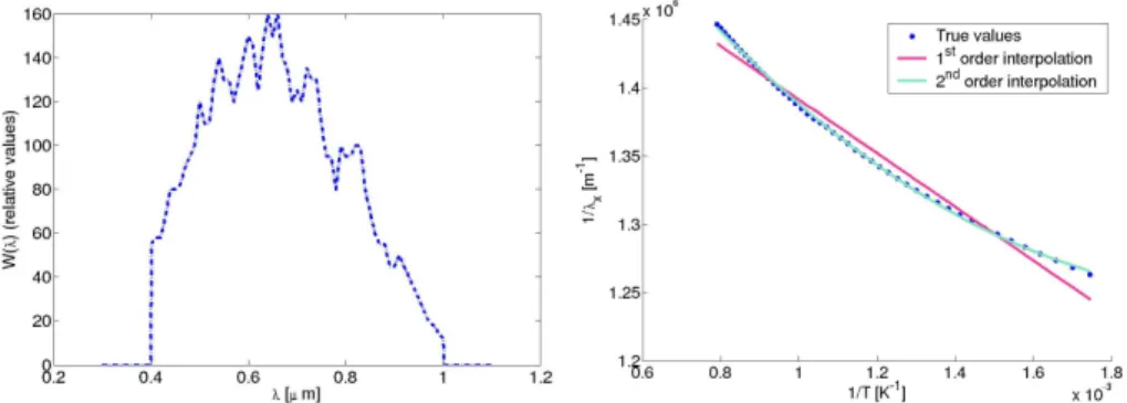
(figureFigure 2. Left: Measurement of W(λ). Right:
λ
x(T
)
and different interpolations.The relation between
λ
x(T) and T can be “tabulated” for different temperatures(from [9] and W(
λ
)) or described by a semi-empirical analytical equation as:... ) ( 1 2 2 1 0+ + + = Ta T a a T x
λ
[10]The number of terms that we should use depends on the amplitude of the temperature range, for a given W(
λ
) function. To evaluate the precision that we can obtain for a given number of terms, we measure the relative W(λ
) function for the dedicated camera used, and we do the following process:- From measured W(
λ
), kw is first evaluated (relation [8]) andλ
x(T) isdetermined for a set of temperatures (relation [9]).
- Using [7], kw and
λ
x(T), Id(T) is calculated; thus providing the referenceoutput signals.
- Next the error between the reference values and those obtained using [7] and [10] with a given number of terms is evaluated.
We note that for a temperature range of 300 - 1000°C, the use of a linear (first order) expression for 1(1)
T x
λ leads to a maximal error of 1.6% on λx, or 21°C of
error at 1000°C. With a second order expression, the error is less than 0.2%, or 2.5°C at 1000°C, which seems to be less important than other sources of imprecision. So we consider that when the system is equipped with a filter and used on a very large temperature range, the second order expression is sufficient. For a 400 - 700°C range, the first order is sufficient as we will see further.
To conclude :
- To realize accurate measurements between 300 and 700°C, we use the relation [7], with
λ
x(T
)
given by the first ordered relation [10].- This relation is correct for a single detector with a linear photo response. These two assumptions will be discussed in the two next sections, regarding respectively CCD and CMOS silicon FPA.
Additionally, we have realized an efficient identification procedure of (kw,a0,a1), from data Id(T) and without knowing of W(
λ
), which is presented in the section 3. Keep in mind that least-square method suffer from problem of conditioning and need a lot of calibration points.2.4. CCD silicon FPA corrections
In this part we examine phenomena that should be corrected to obtain accurate measurements.
2.4.1. Correction of the non linearity of the photo-response
It has been assumed that the output signal is given by [11], i.e. that it is proportional to the energy received during the integration time. In other words, the output signal is proportional to the integration time and to the incident flux.
∫
=Kti W
λ
Lλλ
T dλ
Id0 . . ( ). 0( , ). [11]
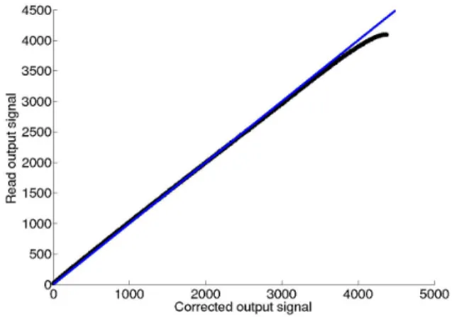
CCD cameras that we studied do not feature a strictly linear photo-response, as we can see on the figure 3. This is due to the fact that commercially “video” cameras are tools for visualization, and not radiometric measurement. To obtain better visualization and particularly to minimize effects of saturation and blooming, detectors are equipped of an anti-blooming system. When the detector is highly illuminated, these drains positioned near the photosensitive area drives the excess signal charges into the substrate. This reduces the effects of blooming, but introduces some non-linearity. (see (Stevens, 1991) for a typical modeling of the linearities). Other causes of linearity are the “Floating diffusion non-linearity”, because the value of the floating diffusion capacitance depends on its amount of charge, or “MOSFET linearity”, related to the on-chip amplifier non-linearity. Both have similar effects.
The proposed approach to take the non linearity into account consists in determining the photo-response of the detector, and generating a function of correction: ) ( 1 0 f Id Id= − [12]
where f is the photo-response of the system, Id is the read output signal and 0
d I is the corrected output signal, proportional to the integration time and the incident irradiance. The photo-response f is determined by preliminary measuring the
digital output signal camera I versus the integration time d ti. Note that during this
measurement, the intensity of the hot source in front of the detector is constant. It is chosen to allow to record output signal on the whole range, from about three times the noise standard deviation (low integration time) to detector saturation (high integration time). We observe a field of linearity FoL (typically from three times the noise standard deviation to the half saturation output signal) where Id is
proportional to ti.By extension we define for all ti:
ti ti Id I FoL d=∂∂ × ) 0 [13]
This relation allows to define, using the preliminary Id(ti), a rate of read charges (see figure 3):
ti
ti
Id
Id
I
Id
Id
C
FoL d×
∂
∂
=
=
) 0)
(
[14]Figure 3. Error of non linearity, here denoted
transfer rate vs. output signal (EC1380).
Physical considerations and experimental measurements show that this rate depends only on the number of generated charges or the signal 0
d
I
, what allows to define, for all irradiance and integration time:)
(
)
(
1 0Id
C
Id
Id
f
I
d=
−=
[15]This correction is coherent with (Stevens, 1991). We observe that the function
) ( 0
d I
f does not depend on the incident spectral distribution.
We see on the figure 3 that the non-linearity reaches 7%, what causes an
error of 10 K at 1273 K. We should correct such a deviation.
Figure 4. Photo response of the CCD EC1380 camera: read
output signalId vs. corrected output signal 0
d
I , in Gray Levels.
2.4.2. Correction of the inter dependence of the detectors and smearing
Four phenomena make the output signal of two or more pixels of the detector array being cross-correlated: the blooming, the smearing, the optical reflections and the diffusion of the generated charges in the substrate of the detector.
The blooming results from of the overexposure of one or many pixels, leading to vertical or horizontal streaks. We adapt during the measurements the integration time to avoid the overexposure of any detector, and so blooming does not affect our images.
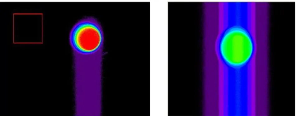
The smearing (see figure 5) is due to the reception of photons during the transfer and/or the read out of the generated charges. It is characterized by the appearance of streaks which depends on the incident irradiance and the number of detectors highly illuminated in the column or the row, but does not depend on the integration time. Its physical causes depend of the architecture of the detector; they are described in (Theuwissen, 1995). The better way to avoid smearing is to use a mechanical shutter, which protect the detector against incident radiation during the transfer and the reading of the charges. But the use of very short integration times (down to 100 µs) prevent from using mechanical shutters. Then we should post-process the images, and two main corrections are possible. The first one consists to block the light for some rows (if the smear creates vertical streaks). Then the variation of offset of these “black” detectors is totally due to smear, and this variation is
subtracted to all detectors of the column. But this system is not implemented in commercial cameras and so we use another algorithm, based on a technique proposed by (Powell et all, 1999). These algorithms have been studied for frame-transfer detector, and we work to adapt them for the used interline architecture.
It is sometimes possible to suppress the smearing by reducing the aperture of the objective, but this increases the minimal temperature of detection. Finally, the smear decreases the amplitude of the temperature range that we can observe, even if we can propose some algorithm of correction when the offset due to smear is not the preponderant signal.
The reflections in the objective, also called “ghost images” (see (Tarel, 1995) and figure 6) cause a lower error that we can neglect. With traditional objectives, the coefficienet of reflection reaches typically 2%, for all wavelengths.
Figure 5. Observation of a circular black body and smearing. On the left:
first illuminated image in which a half spread is observed; on the right: a entire spread, observed without mechanical shutter.
Figure 6. Observation of a black body and of its
Lastly, the charges which are generated by NIR long wavelength photons are created deep in the substrate and diffused in neighbors detectors until they are captured. This leads to a loss of spatial resolution which is presented in (Sentenac et al., 2003).
2.4.3. Non uniformity correction
As we use multi-detectors arrays, we have to take into account that all the detectors are not strictly identical. We characterize the matrix with Fixed Pattern Noise, and Photo-Response Non Uniformity. The point is to eventually correct particular detectors, in order to apply a single radiometric model all over the matrix. We use Calibration based Non Uniformity Correction and proceed like (Healey et al., 1994).
For CCD cameras, we generally do not observe significant variations of properties. For example the figures 7 represents the FPN and the dark current matrix of the EC1380 sensor. Even if we observe a strange vertical streak on the left part of the image, the difference of intensity is less than 3 Gray Levels and may eventually be neglected. The PRNU is measured for different wavelengths and does not present particular pattern.
Figure 7. FPN [Gray Level] and dark current [GL/s] map of the EC1380.
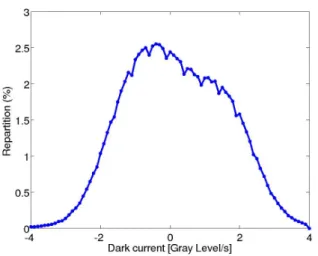
In fact there are only a little bit of detectors which show a particular behavior. For example, 99.8% of the detectors of the matrix admit a dark current less than 4 Gray Levels/s. (see the repartition in figure 8). Then the 0.2% of others detectors can be defined as “wrong” detectors or often “hot” detectors. Their values are not used, and can eventually be replaced by an average value based on their neighbors.
Figure 8. Spatial repartition of the dark current (EC1380).
2.4.5. Radiometric model, for a silicon CCD FPA: summary
The different steps for setting up the radiometric model, for a silicon CCD FPA, can be summed up as follows:
- Photo-response non linearity correction.
- Correction of the smear effects. The value of the ‘wrong’ detectors are suppressed and eventually replaced by an average of the values of their neighbors.
- Application of the radiometric model [7] and [10].
2.5. CMOS Silicon FPA corrections
Smearing effect can also be avoided by using CMOS based silicon FPA, intrinsically resistant to this phenomenon. We evaluate this architecture as an alternative to CCD silicon FPA.
Using CMOS FPA in measuring high temperatures presents an important advantage dealt with the smearing. As there is no transfer of charge with this technology, the offset due to smear affects only the detector highly illuminated, and not all the detectors of its column. So obviously no streak does appear. The correction is individual, and the importance of smearing does not cumulate the
effects of all the highly illuminated detectors of a column. We can observe a
typical smear effect (the offset increases with high flux) for higher temperatures than for CCD.
Figure 9. Evolution of the spatial repartition of the dark current for a
CMOS camera, with the temperature of the detector (20 and 29°C).
Figure 10. PRNU of the CMOS CV1280 camera, at λ=880 and 930 nm.
The main disadvantages of the CMOS FPA concerns their non uniformities. This need a precise characterization. Key point are that the dark currents are higher than these of CCD FPA (that is a well-known fact presented for example in Magnan, 2003), that their distribution is larger and varies quicker with the temperature detector (see figure 9). So the dark currents should be modeled and taken into account, and notably during the measurements of of low temperature (longer integration times). And last the photo response non uniformity (PRNU) must be taken into account (see figure 10), because the differences of sensibility can reach up to 20%, which causes 25°C of error at 1000°C. Unhappily we have noted that the PRNU is highly dependant of the wavelength, and even if the received energy increases quickly with the wavelength, it is not sure that the behavior of the system is accurately described by the PRNU at a given wavelength.
CMOS silicon FPA are promising for measuring high temperature, but the temperature of the detector need to be controlled, and the characterization of the FPA is more specific.
3. Calibration procedure
In this part, the calibration procedures are detailed. The silicon FPA one is a very short process, with accurate performances and an identification of parameters without initialization.
3.1. Calibration set up
The experiment takes place in a dark room at a stable temperature. It is composed of a reference source viewed directly by the camera. The used reference source is a P-1200 blackbody manufactured by Land Infrared. Its emissivity is 0.998 and its aperture is 54 mm. The studied temperature range is 400 - 700°C.
The infrared cameras are manufactured by Agema. 0ne is the 780 camera, equipped with an InSb mono-detector (3 − 5 µm) cooled at 77 K and the other is the 880 LWB camera with an HgCdTe mono-detector (8 − 12 µm), cooled at 77 K with a Stirling cycle. Their usual frame rate is 6 images per second. The CCD silicon FPA is the Prosilica EC1380.
The alignment blackbody-camera is provided by an optical bench. The distance between blackbody-camera is fixed at 1.2 meter.
3.2. Traditional calibration process
The calibration of IR cameras, or silicon FPA in other works (for example Meriaudeau et al., 2003) are characterized by many measurements at different temperatures. A non linear identification needing a precise initialization of the set of parameters is applied.
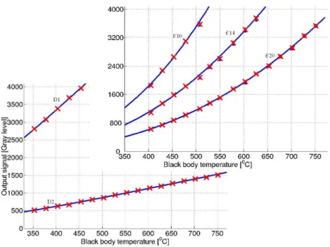
Here, for the infrared cameras, we do acquisitions from 400 to 750°C, with an increment of 25°C, for each f-number. Each of these acquisitions (Id, T) is an average on one hundred images, to remove temporal noises. The results are shown in figure 11 and section 4.1.
Here is a set of parameters for the MWIR camera: N = 10; A = 3.00 GL;
Figure 11. Experimental results for the infrared cameras.
3.3. Specific calibration process
For silicon FPA, the first step is the determination of the photo response of the detector, as described in §2.3.1.
Then, only three measurements at high temperatures (600, 650 and 700°C) are
needed to find
k
w and the parameters which defineλ
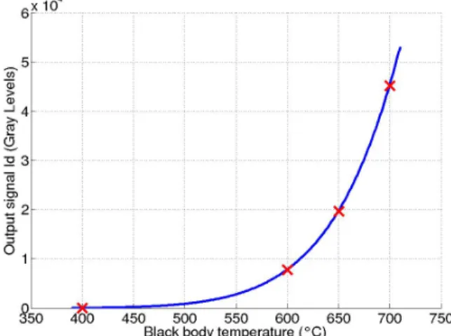
x(T). So the calibrationprocedure is very short. For each temperature, we acquire a temporal average of the intensity on two regions of interest, one corresponding to a uniform region of the black body, and a second which is on the same columns, in a non illuminated region; that allows to estimate the offset due to smear. More precisely, we acquired for each temperature different values of Id for different integration times; this is a very short process, which allows to estimate more precisely the output signal and provides a response in Gray Levels per second (see figure 12).
To determine the value of the set of parameters, we have shown the efficiency of the following process: over a small temperature range, we know that
T a a x1= 0+ 1 −
λ
.For a given amplitude of the temperature range, this approximation is more true when the temperature is higher. So we consider the three higher points (Id, T), here at 600, 650 and 700°C. These three points provide three relations [17] and so values of the three parameters
k
w,a
0anda
1:) .( ) ln( ) ( . ) ln( ) ) ( ln( 0 12 2 2 0 i i w i x i w i d Ta T a C k T T C k tiT I = − = − +
λ
[17]For the 400-700°C temperature range, this step is sufficient. The 400°C measurement only provides the confirmation of the fitness of the model (see next section).
Its parameters are: kw = 2.12 e11 GL/s; a0 = 1.10 e6 m-1 and a1 = - 3.02 e7 m-1K-1.
Figure 12. Normalized calibration curve of the
EC1380 camera, for an integration time of 1 second.
4. Comparison of performances
This section describes the results of the comparison between two IR cameras and the CCD silicon FPA. These three cameras provide a 12 bit signal per pixel. First, we introduce some criteria to characterize the parameterized radiometric models. Next, intrinsic performances such as sensitivity and Noise Equivalent Temperature Difference (NETD) are compared. Finally, we introduce some information dealing with the true temperature measurements.
4.1. Evaluation of the radiometric models
We define three criteria intended to evaluate the performances of the radiometric models : the trueness, the precision, and the maximal error. We evaluate and compare these criteria for each camera. Note that such criteria are not only used to compare different systems, but also serve in study and identification of potential
“problems”. It is indeed possible to estimate this criteria on only a part of the set of calibration points and that may show some interesting phenomena; for example the non linearity of the photo response was pointed out by noting that the trueness was smaller for higher output signals.
4.1.1. Definitions
We consider the set of calibration data (Id, T) and we note E[x] the mean value of x. Otherwise we note Tˆ the estimation of T provided by the radiometric model,
knowing Id.
Then the trueness J of the parameterized model is defined (Perruchet et al., 2000):
] ˆ [ 1 T T E J − = [19]
The precision F and the maximal error Emax are defined as:
] ) ˆ [( 1 2 T T E F −
= and Emax=max(Tˆ−T)
[20]
4.1.2. Results
The next table summarizes results for different configuration of the three cameras. For the three cameras, the considered set of data is the mean output signal on the region of interest.
Model N 1/J (°C) 1/F (°C) Emax(°C) 10 1.0 2.7 4.6 MWIR 14 1.4 3.4 6.4 20 0.4 1.7 3.8 LWIR (D1) 0.1 1.2 2.0 LWIR (D2) 0.1 3.8 7.3 NIR - 0.1 0.2 0.5
4.2. Intrinsic performances 4.2.1. Sensitivity
The on-line adaptation of the integration time (see Rotrou et al., 2005) for a description of the algorithm) allows to optimize the sensibility of the system, but leads to use a great number of integration times.
The sensitivity of the system is traditionally defined as ( 0
d
I
Id
=
for IR cameras): T T Id T S ∂ ∂ = ) ( [21]For infrared systems using the radiometric model [6], it can be analytically computed: 2 2.( .exp( / ) 1) ) / exp( . . . ) (T =ABCT C BBTT − S [22]
Figure 13. Sensitivity [Gray Levels / °C].
For the silicon FPA, we consider firstly the corrected signal 0
d
I , and the extended effective wavelength defined at the first order (see [17]).Then we obtain a maximal sensitivity S0(T) in the next relation, where 0
d
I is maximal by adapting the integration time:
) . 2 .( . ) ( 31 2 0 2 0 0 Ta Ta C I T S = d + [23]
This is a maximal sensitivity which is not really obtained. Indeed if we consider that 0
d
I is not the read output signal but a corrected signal due to the non linearity of the photo response, we should take into account this photo response f. The relation :
) ( . . ) ( ) ( 0 0 0 0 0 0 0 T S I f T I I f T I f T Id T S d d d I d I d T d T ∂ ∂ = ∂ ∂ ∂∂ = ∂ ∂ = ∂ ∂ = [24]
shows that the loss of sensitivity is easily linked to the loss of sensitivity of the photo-response. Here the higher loss is 7%.
If there are smear effects, the sensitivity indirectly decreases; indeed, as the smear creates an artificial offset, we should decrease the integration time to not saturate, thus 0
d
I then S0(T)and S(T) would decrease too.
Anyway, it appears that silicon FPA are promising and can present a better sensitivity than infrared systems. We should lastly note that the sensitivity varies quickly with the temperature; that means that it is not constant in an image with thermal gradients, and that we can not assure that very good sensitivity for all the image if it is very contrasted.
4.2.2. Generalized NETD
The Noise Equivalent Temperature Differences NETD is defined as the ratio of the standard deviation noise to the sensitivity. It is computed for Signal Noise Ratio equal to 1 and a temperature of 30°C. As 30°C is not a detectable temperature with silicon detectors, we can not compare the systems.
We propose to generalize the notion of NETD by introducing the temperature of the black body that we observe. So the GNETD – G for generalized -, at the black body temperature T, is the ratio of the standard deviation noise to the sensitivity, both considered for the temperature T. In figure 14, we present result considering that the standard deviation is constant and unitary. Found values for IR detectors are comparable with values given by the manufacturer.
Regarding the emissivity of a real material, we know that the measurement is less sensitive to the uncertainty of the emissivity – or its spatial variation -, at lower wavelengths. Indeed considering a monochromatic measurement, we see that the uncertainty dT on the measured temperature due to the uncertainty dε on emissivity is proportional to the wavelength:
ε
ε
λ
d
C
T
T
dT
.
.
2−
=
[25]Figure 14. GNETD supposing the noise is constant and unitary.
For a given state of surface (
d
ε
), the uncertainty dT is about 10 times less important in the NIR than in the LWIR (see figure 15). A study published in (Rotrou et al., 2005) shows that the error on the NIR image of a mould is less than 3°C (between 300 and 520°C). During the cooling of the mould, gradients of temperatures appear due to its shape. These gradients (few dozen of degrees) areFigure 15. On the left, observation of a real surface with LWIR camera and, on
the right, NIR camera. On the left, we see more spatial variations of emissivity than temperature gradients. On the right, isotherm curves are really observed.
shown on the NIR image. On the LWIR image, the differences of apparent temperature are higher (more than one hundred degrees) and so they are not due to the cooling of the mould. The observed gradients come from gradients of emissivity.
4.3. True temperature measurement
In this last part we introduce some notes about the measurement of true temperature. Indeed the radiometric model allow to obtain black body temperature, or the incident flux. Some external factors must be taken into account to access to the true temperature of the observed object: the emissivity of the material, the temperature of the air, the shape of the object which determines the relation between radiance and emitted fluxes.
5. Conclusion
In this paper, we present a general radiometric model of a silicon FPA. We compare its performances with those of two commercial MWIR and LWIR cameras.
One of the originalities of the work is that only one set of parameters is determined for all integration time. The study leads to an easy-to-use and effective calibration procedure, without tedious measurement of W(λ).
The comparison with two commercial infrared cameras shows that silicon FPA properties are promising. Thanks to the real time control of the integration time, the sensitivity of our system reaches more than 60 Gray Levels by degree and offers values higher than the sensitivities of infrared cameras. The Generalized NETD of these three systems, introduced as a new metric, are comparable, around 0.1°C. Additionally, as it works at shorter wavelengths, our system offers the advantage of being less sensible to the emissivity of the material. So its use is particularly recommended, for example, in the study of non uniform materials (e.g. forming moulds, metallic steels with degraded state of surface…), and other applications requiring good spatial resolution.
Finally, we demonstrate with this work that silicon FPA complement the large range of thermographic systems commercially proposed. Further investigations are pursued, with CMOS silicon FPA.
6. References
Healey G.E. and Kondepudy R., “Radiometric CCD camera calibration and noise estimation”,
IEEE Transactions on Pattern Analysis and Machine Intelligence, Vol. 16, no. 3, pp.
Kostkowsky H.J. and Lee R.D., Theory and Method of Optical Pyrometry, Reinhold Publishing Corporation, 1962.
Magnan P., “Detection of visible photons in CCD and CMOS: A comparative view”, Nuclear
Instruments and Methods in Physics Research, Vol. 504, pp 199-212. May 2003.
Mériaudeau F., Legrand A.C. and Gorria P., “Real Time Multispectral High Temperature Measurement: Application to control in the industry”, Machine Vision Applications in
Industrial Inspection XI, SPIE Vol.5011, 2003.
Perruchet C. and Priel M., Estimer l’incertitude, AFNOR 2000.
Powell K., Deeph C., Fish D. and Thompson C., “Restoration and frequency analysis of smeared images”, Applied Optics, Vol. 38, no.8, pp.1343-1347, 1999.
Pron H. and Bissieux C., “Focal plane array infrared cameras as research tools”, QIRT
Journal, Vol.1, no.2, pp. 229-240, 2004.
Rotrou Y., Sentenac T., Le Maoult Y., Magnan P. and Farré J., “Demonstration of near-infrared thermography with silicon image sensor camera”, Thermosense XXVII, SPIE
Proc. Vol. 5782, pp. 9-18, 2005.
Saunders P., “General interpolation equations for the calibration of radiation thermometers”,
Metrologia, Vol.34, pp. 201-210, 1997.
Sentenac T., Le Maoult Y., Orteu J-J. and Boucourt G., “Evaluation of a charge-coupled-device-based video sensor for aircraft cargo surveillance”, Optical Engineering 41(4), 2002
Sentenac T., Le Maoult Y., Rolland G. and Devy M., “Temperature correction of radiometric and geometric models for an uncooled CCD camera in the near infrared”, IEEE
Transactions on Instrumentation and Measurement Journal, Vol. 1, 2003.
Stevens E.G., “Photoresponse Nonlinearity of Solid-State image Sensors with Antiblooming Protection”, IEEE Transactions on Electron Devices, Vol. 39, no. 11, 1991
Tarel J-P., “Calibration radiométrique de cameras”, Rapport technique 2509, INRIA, 1995 Theuwissen A., Solid-state imaging with charge-coupled devices, Kluwer Academic


![Figure 7. FPN [Gray Level] and dark current [GL/s] map of the EC1380.](https://thumb-eu.123doks.com/thumbv2/123doknet/11585703.298355/13.892.203.701.585.776/figure-fpn-gray-level-dark-current-gl-map.webp)