Publisher’s version / Version de l'éditeur:
Vous avez des questions? Nous pouvons vous aider. Pour communiquer directement avec un auteur, consultez la première page de la revue dans laquelle son article a été publié afin de trouver ses coordonnées. Si vous n’arrivez pas à les repérer, communiquez avec nous à [email protected].
Questions? Contact the NRC Publications Archive team at
[email protected]. If you wish to email the authors directly, please see the first page of the publication for their contact information.
https://publications-cnrc.canada.ca/fra/droits
L’accès à ce site Web et l’utilisation de son contenu sont assujettis aux conditions présentées dans le site LISEZ CES CONDITIONS ATTENTIVEMENT AVANT D’UTILISER CE SITE WEB.
Indoor Air 2008, The 11th International Conference on Indoor Air Quality and Climate [Proceedings], pp. 1-7, 2008-08-16
READ THESE TERMS AND CONDITIONS CAREFULLY BEFORE USING THIS WEBSITE.
https://nrc-publications.canada.ca/eng/copyright
NRC Publications Archive Record / Notice des Archives des publications du CNRC :
https://nrc-publications.canada.ca/eng/view/object/?id=dee89feb-1906-4718-8982-e93b31144351 https://publications-cnrc.canada.ca/fra/voir/objet/?id=dee89feb-1906-4718-8982-e93b31144351
NRC Publications Archive
Archives des publications du CNRC
This publication could be one of several versions: author’s original, accepted manuscript or the publisher’s version. / La version de cette publication peut être l’une des suivantes : la version prépublication de l’auteur, la version acceptée du manuscrit ou la version de l’éditeur.
Access and use of this website and the material on it are subject to the Terms and Conditions set forth at
Can long-term emissions be predicted with models based on short-term emissions?
http://irc.nrc-cnrc.gc.ca
C a n l o n g - t e r m e m i s s i o n s b e p r e d i c t e d w i t h
m o d e l s b a s e d o n s h o r t - t e r m e m i s s i o n s ?
N R C C - 5 0 8 0 3
W o n , D . ; Y a n g , W . ; M a g e e , R . J . ; S c h l e i b i n g e r ,
H .
A version of this document is published in / Une version de ce document se trouve dans: Indoor Air 2008, 11th International Conference on Indoor Air Quality and Climate, Copenhagen, Denmark, Aug. 16-22, 2008, pp.1-7
The material in this document is covered by the provisions of the Copyright Act, by Canadian laws, policies, regulations and international agreements. Such provisions serve to identify the information source and, in specific instances, to prohibit reproduction of materials without written permission. For more information visit http://laws.justice.gc.ca/en/showtdm/cs/C-42
Les renseignements dans ce document sont protégés par la Loi sur le droit d'auteur, par les lois, les politiques et les règlements du Canada et des accords internationaux. Ces dispositions permettent d'identifier la source de l'information et, dans certains cas, d'interdire la copie de documents sans permission écrite. Pour obtenir de plus amples renseignements : http://lois.justice.gc.ca/fr/showtdm/cs/C-42
Can long-term emissions be predicted with models based on short-term
emissions?
Doyun Won*, Wenping Yang, Robert Magee, and Hans Schleibinger
Institute for Research in Construction, National Research Council Canada, 1200 Montreal Road, Ottawa, Ontario K1A 0R6, Canada
*
Corresponding email: [email protected]
SUMMARY
Standard tests for volatile organic compound emissions from construction materials and furniture typically last less than a week. The short-term data are often used to predict long-term emissions. The validity of the extrapolation from the short-long-term experimental data to long-term predictions was investigated. A dynamic chamber test was conducted continuously for over a year to obtain concentration versus time data for chemical emissions from an oriented strand board specimen at controlled conditions. The coefficients of a power-law type emission model were estimated using the short-term data (up to 1 week). The model was used to predict long-term emissions (up to 1 year). The performance of short-term models deteriorated as they were extrapolated to predict longer-term emissions. Extrapolating emission data beyond the testing period can introduce a high level of uncertainties and should be done with caution. Information on potential errors should be provided when simulation results are presented.
KEYWORDS
Material emissions, Volatile organic compounds, Long-term emissions, Oriented strand board, Chamber testing
INTRODUCTION
To predict indoor air concentrations of volatile organic compounds (VOCs), it is necessary to know the emission characteristics of building materials, which are major sources of these chemicals indoors. Small-scale chamber testing, the most frequently used method for source characterization of indoor materials, has been standardized through development of international guides such as ASTM Standard D5116 (ASTM, 2006). While there is no limit to the duration of chamber testing, one test typically lasts from 3 days to 28 days (BIFMA, 2006; California Department of Health Services, 2004; European Commission, 2005). The concentration versus time data from a short-term chamber test is used to obtain emission factors and consequently emission models (BIFMA, 2006).
Although it is well recognized that such models, in particular, empirical models, are applicable only within the range of measurements, the models based on short-term measurements are frequently extrapolated to predict long-term emissions. Since this extrapolation of empirical models based on short-term measured data is common, it is important to determine the accuracy of the long-term predictions.
With a few exceptions (Hodgson et al., 2004; Magee et al., 2002; Zhu et al., 2001) there has been very little research on these extrapolation issues associated with material emissions and indoor air quality (IAQ). The goal of this work is to investigate whether empirical emission
models based on short-term chamber testing can predict long-term emissions with acceptable accuracy.
METHODS Chamber testing
A chamber test was conducted on a specimen of oriented strand board (OSB6a). Specimen preparation and chamber test procedures followed the recommendations in ASTM Standard D5116. Oriented strand board was chosen because it is widely used in the construction. Air samples were taken on 2,4-dinitrophenylhydrazine (DNPH) cartridges for carbonyl compounds including formaldehyde, acetaldehyde, propanal, butanal, pentanal, and hexanal. The DNPH cartridges were extracted with acetonitrile and analyzed by a High Performance Liquid Chromatography (Varian 9012 Solvent Delivery System / 9050 Variable Wavelength UV-VIS Detector at 360nm).
Empirical modeling
Chamber air concentrations were predicted based on the mass balance equation applied to the chamber system (Eq. 1).
EF A C Q t d C d V =− + (1)
where V is chamber volume (m3), Q is chamber flow rate (m3/h), A is surface area of the specimen (m2), and EF is emission factor (ug/m2/h).
According to Zhu et al. (2001), a power-law equation predicted long-term emission factors (up to 900 hours) better than an exponential decay model for wood-based panels. Therefore, Eq. 2 was used to describe the change of emission factors over time.
(2) 2 1 a t a EF = −
where a1 and a2 are empirical constants, and t is time (h).
Assuming that a steady state can be achieved at longer times, Eq. 1 and Eq. 2 can be simplified to Eq. 3. The equation was used to fit to the short-term data (between 24 hours and 1 week) to obtain best-fit coefficients of a1 and a2 using Excel.
2 1 a t a N L C= − (3)
RESULTS
Chamber conditions
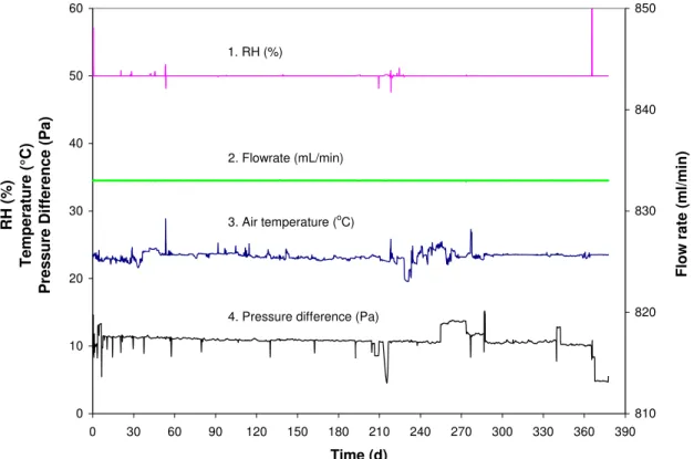
Figure 1 summarizes the environmental conditions of the test chamber for the OSB specimen. The data were recorded every minute and were averaged every four hours for plotting. The chamber flow rates (Q) and relative humidity (RH) were precisely controlled through mass-flow controllers continuously monitored by a dedicated data acquisition and control system, which was connected to an uninterruptible power supply (UPS). Temperature (T) control (at a target value of 23 ± 0.5 oC) was provided with a separate HVAC system for the test laboratory (this system was, however, despite redundant back-up chillers, dependent on the building’s chilled water system and on the main building power). Both the chilled water and electrical power systems experienced brief failures during the course of the year-long test and are reflected in the transient temperature spikes observed.
The chamber was designed to operate at a very slight positive pressure (10 Pa or ~ 0.04 inches of water) to prevent contamination of the test environment. Figure 1 shows that this positive pressurization was maintained and was generally within a few pascals of the target pressure (the brief drops in pressure occurred due to sampling from the chamber exhaust, but indicate that chamber pressurization remained slightly positive during these times). The relative humidity profile shows two brief spikes to 57 – 60 % at the beginning and end of the test. The cause of these spikes has not been determined. The coefficient of variance (CV) of the four-hour average data is 5.16E-6 (flow rate), 0.03 (temperature), 0.088 (RH), and 0.12 (pressure difference). The low values of CV confirm that the environmental conditions in the chamber were very well-controlled.
0 10 20 30 40 50 60 0 30 60 90 120 150 180 210 240 270 300 330 360 390 Time (d) RH (%) Temperature (°C)
Pressure Difference (Pa)
810 820 830 840 850
Flow rate (ml/min)
1. RH (%)
2. Flowrate (mL/min)
3. Air temperature (oC)
4. Pressure difference (Pa)
Empirical modeling
Table 1 shows the curve-fitting results for the short-term data. The R2 values indicate that the power-law model fit the short-term emission data very well except for formaldehyde.
Table 1. Coefficients of empirical models for the short-term data
Chemicals a1 a2 R2 Formaldehyde 17.96 0.1175 0.4956 Acetaldehyde 719.67 0.3395 0.9549 Propanal 171.16 0.2411 0.9485 Butanal 69.47 0.1555 0.8890 Pentanal 2059.10 0.6234 0.9901 Hexanal 4890.10 0.4631 0.9410
Figure 2 and Figure 3 compare the measured long-term data (between 1 week and 1 year) with the predicted data based on short-term models (between 24 hours and 1 week). Between 1 week and 1 month, there is no general trend: good agreement for hexanal, under-prediction for pentanal and propanal, and over-prediction for formaldehyde, aldehyde, and butanal. On the hand, the long-term emissions after 2 months tend to be over-predicted by the short-term model. The over-predicted concentrations are more pronounced with hexanal, acetaldehyde, and propanal. There is about a factor of 10 over-prediction for acetaldehyde and propanal and a factor of 5 over-prediction for hexanal around 1 year. While the concentrations of formaldehyde and butanal are over-predicted, the maximum difference is about a factor of two. One exception to over-prediction is pentanal, which shows good agreement after 5 months. 0.1 1 10 100 1000 0 30 60 90 120 150 180 210 240 270 300 330 360 390 Time (d) Air c onc e n tra tion ( ug/m 3 ) Formaldehyde (measured) Formaldehyde (predicted) Pentanal (measured) Pentanal (predicted) Hexanal (measured) Hexanal (predicted)
Figure 2. Comparison of measured and predicted chamber concentrations (formaldehyde, pentanal, and hexanal).
0.1 1 10 100 0 30 60 90 120 150 180 210 240 270 300 330 360 390 Time (d) Air c onc e n tra tion ( ug/m 3 ) Acetaldehyde (measured) Acetaldehyde (predicted) Propanal (measured) Propanal (predicted) Butanal (measured) Butanal (predicted)
Figure 3. Comparison of measured and predicted chamber concentrations (acetaldehyde, propanal, and butanal).
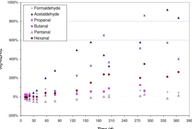
-200% 0% 200% 400% 600% 800% 1000% 0 30 60 90 120 150 180 210 240 270 300 330 360 390 Time (d) (C p -C m )/C m Formaldehyde Acetaldehyde Propanal Butanal Pentanal Hexanal
Figure 4. Relative differences between measured and predicted chamber concentrations for aldehydes.
Figure 4 shows the relative differences between measured (Cm) and predicted (Cp) concentrations. The relative differences tend to increase over time. For example, the relative difference for acetaldehyde increased from 5 % at 14 d to 42 % at 30 d, to 200 % at 60 d, and to 837 % at 365 d. For all six compounds, the relative difference between Cm and Cp ranges from –30 % to 30 % for the two-week extrapolation, from –52 % to 42 % for the one-month extrapolation, from –52 % to 200 % for the two-month extrapolation, and from –27% to 500 % for the 4 month extrapolation.
DISCUSSION
This study shows that it is not easy to generalize the prediction capabilities of a short-term model for long-term emissions even for chemicals within one class such as aldehydes. One example is that predictions are relatively poor at the early extrapolation, but they improve as the extrapolation is extended to a longer period (e.g., pentanal). Another example shows that the prediction errors caused by extrapolation are in a relatively constant level over one year (e.g., formaldehyde). However, the most common observation is that the prediction errors increase over time as extrapolation is extended to a longer period. This study shows that it is more likely that extrapolation of short-term data can introduce a large amount of uncertainties and the uncertainties can get bigger for longer-term predictions.
Although the method to determine emission models is often discussed in material emission testing protocols (e.g., ASTM D5116), there is not much information on the potential errors that can be caused by extrapolation of short-term emission data. One example is the standard test method by the Business and International Furniture Manufacture’s Association (BIFMA, 2006), which suggests that power-law models based on 7-day testing can be used to predict concentrations for early occupancy time points (e.g., 14 days). While there is a brief mention on measurement errors, no indication is given for the consequence of the extrapolation. While it is conceivable that estimations based on models are associated with errors, it is important to understand the magnitude of the errors. This is particularly important when simulation tools present estimated results. It is highly encouraged to show potential error bounds associated with simulated values or to use a probabilistic concept in simulations.
This study, which shows one example of extrapolation based on 1-week data, can be expanded in many ways. First, it can be interesting to see how the error changes if other time periods are used as short terms. One example is 28-day, which is the second testing period in addition to 3-day testing in many European labelling schemes (European Commission, 2005). This type of analysis may be able to shed light on the required testing period for a material emissions test if one is interested in extrapolation with a particular level of uncertainties. Secondly, the study is done for several aldehydes based on DNPH-cartridge sampling and HPLC analysis. Similar analyses can be extended to other VOCs that are better analyzed with sorbent tube-sampling and gas chromatography/mass spectrometer (GC/MS) analysis. This may provide us an idea on whether extrapolation errors can change depending on chemical classes and, therefore, whether different chemicals act differently in term of long-term emissions. Thirdly, the study can be expanded to other building materials. As different building materials have different degrees of homogeneity and availability of chemicals for emissions, this may be able to explain the deviation of long-term emission trend from the short-term in terms of material properties. The authors are planning to expand the analysis to other time periods and chemicals from OSB specimen tests in future publications.
CONCLUSIONS
While this study is limited to six different aldehyde emissions from one OSB specimen, it demonstrates that extrapolating experimental results to longer time periods beyond the testing period can introduce a high level of uncertainties to the emission data from building materials and should be done with caution. For example, it is not uncommon that prediction errors can increase to ~1000 % if the extrapolation is extended to one year from one week. Although simulation tools are not expected to provide precise estimations on VOC levels from building materials, it is important to understand the potential errors associated with simulation results. Further research is recommended to improve the reliability of simulated results based on extrapolation. This can be accomplished through further investigating errors associated with emissions from a broader range of materials, chemicals and testing/simulation periods, and through introducing a probabilistic concept to IAQ simulations.
REFERENCES
ASTM. 2006. ASTM Standard D 5116, Standard Guide for Small-Scale Environmental Chamber Determinations of Organic Emissions From Indoor Materials/Products. West Conshohocken, PA: American Society for Testing and Materials.
BIFMA. 2006. BIFMA M7.1-2006, Standard Test Method for Determining VOC Emissions From Office Furniture Systems, Components and Seating. BIFMA International.
California Department of Health Services. 2004. Standard Practice for the Testing of Volatile Organic Emissions From Various Sources Using Small-Scale Environmental Chambers. European Commission. 2005. Report No 24, Harmonisation of Indoor Material Emissions
Labelling Systems in the EU, Inventory of Existing Schemes.
Hodgson A.T., Shendell D.G., Fisk W.J., and Apte M.G. 2004. Comparison of predicted and derived measures of volatile organic compounds inside four new relocatable classrooms.
Indoor Air, 14(s8), 135-144.
Magee R.J., Bodalal T.A., Biesenthal T.A., Lusztyk E., Brouzes M., and Shaw C.Y. 2002. Prediction of VOC concentration profiles in a newly constructed house using small chamber data and an IAQ simulation program. In: Proceedings of The 9th International
Conference on Indoor Air Quality and Climate, Monterey, USA, Vol. 3, pp. 208-303.
Zhu J.P., Zhang J.S., and Shaw C.Y. 2001. Comparison of models for describing measured VOC emissions from wood-based panels under dynamic chamber test condition.