HAL Id: hal-00634305
https://hal.archives-ouvertes.fr/hal-00634305
Submitted on 20 Oct 2011HAL is a multi-disciplinary open access
archive for the deposit and dissemination of sci-entific research documents, whether they are pub-lished or not. The documents may come from teaching and research institutions in France or abroad, or from public or private research centers.
L’archive ouverte pluridisciplinaire HAL, est destinée au dépôt et à la diffusion de documents scientifiques de niveau recherche, publiés ou non, émanant des établissements d’enseignement et de recherche français ou étrangers, des laboratoires publics ou privés.
Computation
Vincent Labatut, Josette Pastor
To cite this version:
Vincent Labatut, Josette Pastor. Dynamic Bayesian Networks for Integrated Neural Computation. 1st International IEEE-EMBS Conference on Neural Engineering, 2003, Capri, Italy. pp.537-540, �10.1109/CNE.2003.1196882�. �hal-00634305�
Abstract-Understanding the clinical outcomes of brain lesions necessitates knowing how networks of cerebral structures implement cognitive or sensorimotor functions. Functional neuroimaging techniques provide useful insights on what the networks are, and when and how much they activate. However, an interpretative method, explaining how the activation of large-scale networks derives from the cerebral information processing mechanisms involved in the function, is still missing. Our goal is to provide such a tool. We suggest that integrated neural computation can be best represented with dynamic Bayesian networks. Our modeling approach is based on the anatomical connectivity of cerebral regions, the information processing within cerebral areas and the causal influences that connected regions exert on each other. We use experimental results [1] concerning the modulation of the striate cortex’s activation by the presentation rate of visual stimuli, to show that our explicit modeling approach allows the interpretation of neuroimaging data, through the formulation and the simulation of functional and physiological assumptions.
Keywords - Computational neuroscience, functional neuroimaging, dynamic Bayesian networks, large-scale cerebral networks
I.INTRODUCTION
The understanding and the prediction of the clinical outcomes of cerebral lesions, as well as the assessment of rehabilitation procedures, necessitate knowing the nature and the functioning of the cerebral substratum of cognitive or sensorimotor functions. In humans, the substratum identification can only be addressed indirectly, through activation studies, where subjects are asked to perform a specific task involving the functions, while data of their brain functioning are collected thanks to functional neuroimaging techniques. It has been shown [2][3] that the functions are the offspring of the activity of large-scale networks of anatomically connected cerebral areas.
Traditional neuroimaging methods allow knowing where [1], i.e. in which areas, and/or when [4] during the task performance, the brain’s activity reaches local maxima. They also give a sketch of what the network of cerebral areas activated is [5], and why the activation of an area can affect another connected cerebral structure [6]. Clearly, they do not answer how the activation derives from the integrated neural computation in large-scale cerebral networks.
Modeling neural computation is at the core of computational neuroscience. Most existing works in the domain are based on formal neural networks, with varying levels of biological plausibility, from physiology-based models [7], hardly interpretable in terms of information processing, to purely functional models [8], not concerned with cerebral plausibility. More recently, Bayesian networks have been used to model visuomotor mechanisms [9], which
demonstrates the utility of graphical probabilistic
formalisms for cerebral functional modeling.
Above methods can hardly both answer the how and provide models explicit enough to be directly used for clinical purpose. In fact, few researches answer the question or meet the necessity [10]. Hereafter, we demonstrate how the interpretation of functional images for a clinical purpose can be tackled. Section II presents our viewpoint on large-scale cerebral networks. After a short introduction to dynamic Bayesian networks, section III describes the characteristics of our formalism. Section IV illustrates the formalism’s capabilities by an example. We conclude with some perspectives.
II. LARGE-SCALE CEREBRAL NETWORKS
A. Structural and Functional Nodes
The function implemented by a large-scale network depends on three properties: the network’s structure [3], the more elementary functions implemented by its nodes (the functional role of each region), and the properties of its links (length, role: inhibitory or excitatory, …).
In each network, regions are information processors and connecting oriented fibers are information transmitters [11]. Each region (structural node) is itself a network of smaller information processors (functional nodes) that are neuronal populations, connected through neuronal fibers, and implement functional primitives (e.g. GABAergic neurons that have an inhibitory role on pyramidal cells). All functional primitives may be different.
A large-scale network has therefore neurophysiologically constrained, oriented edges and possibly differentiated nodes. The explicit representation of the nodes’ function allows the direct expression of hypotheses on cerebral processing, and their easy modification in order to follow the evolution of knowledge in neurosciences. This is not the case of formal neural networks’ implicit modeling approach that requires modifying the whole network architecture to implement functional changes.
Hereafter, a structural or a functional structure will be indifferently named a cerebral zone.
B. Information Representation and Processing
The cerebral information that is processed by a neuronal population can be seen as the abstraction of the number and the pattern of the neurons firing for this information. It can be represented both by an energy level and by a category. Energy is indirectly represented by the imprecise activation data provided by neuroimaging techniques. The category representation is in agreement with the “topical”
Dynamic Bayesian Networks for Integrated Neural Computation
V. Labatut, J. Pastor
organization of the brain, which reflects category maps of the input stimuli, and can persist from primary cortices to nonprimary cortices and subcortical structures [2], through transmission fibers [11]. The energy and the category of a
stimulus can also be easily extracted from its
psychophysical properties.
Modeling cerebral processes necessitates an explicit and discrete representation of time, both for taking into account the dynamics of cerebral mechanisms (transmission delays, response times…), and for complying with sampled functional neuroimaging data.
Since oriented anatomical links provide spatial and temporal contiguity between cerebral nodes, cerebral events are temporally consistent (a firing zone provokes the activation of downstream zones), and there is a statistical regularity in the response of a specific neuronal population to a given stimulus, information processing in a large-scale network can be considered as mediated through causal mechanisms. Those mechanisms, which are the abstraction, at the level of a neuronal population, of the chemical and electrical mechanisms at the cell levels, are often nonlinear.
III. OVERVIEW OF THE FORMALISM
Causal dynamic Bayesian networks are the paradigm that meets best the constraints derived from large-scale networks’ properties.
A. Introduction to Dynamic Bayesian Networks
A causal Bayesian network consists of a directed acyclic graph where nodes represent random variables and edges represent causal relationships between the variables [12]. A conditional probability is associated with each relationship between a node and its parents. If the node is a root, the probability distribution is a prior. When some nodes’ values are observed, posterior probabilities for the hidden nodes can be computed thanks to inference algorithms such as the junction tree algorithm [13].
In a dynamic Bayesian network (DBN), the evolution of random variables through time is considered. Time is seen as a series of intervals called time slices [14]. For each slice, a submodel represents the state of the modeled system. DBNs are used to model Markovian processes, i.e. processes where a temporally limited knowledge of the past is sufficient to predict the future. The choice of the inference algorithm, generally an extension of the junction tree algorithm [15], depends on the DBN’s structure, the nature of its variables (discrete or continuous), and its relationships (linear or nonlinear).
A realistic cerebral modeling necessitates representing continuous values and nonlinear relationships. Furthermore,
although they represent non-neuronal functions,
neuroimaging data, which are the only observable values, must be integrated in our models. Thus, we have a set of hidden variables (the cerebral network) constituting a Markov chain, and a set of observable variables (neuroimaging data) depending only on the hidden variables. Specific algorithms exist for this type of
structures, called a fully nonlinear state space model (SSM). The extended Kalman filter (EKF) is based on Taylor approximations, it needs a linearization, which can lead to unreliable results [16, 17]. The unscented Kalman filter (UKF) is based on the unscented transformation [16], which allows to represent a probability distribution by a set of chosen points, and then to bypass the linearization required by the EKF, and thus to have better performances (more accurate results). The DD1 and DD2 filters [17] use polynomial approximations, offering qualities comparable to the UKF (but more accurate; according to their author [17]). In order to be able to represent nonlinear relationships, the UKF and the DD1/DD2 filters are the most adapted algorithms.
B. Static and Dynamic Networks
A static network is the graphical representation of a large-scale network, whose nodes are cerebral zones and edges are the oriented axon bundles connecting zones. Due to anatomical loops, it is often cyclic. The DBN is the acyclic temporal expansion of the static network. Each node of the DBN is the processing entity related to a cerebral zone, i.e. the mathematical expression, at a given time slice, of information processing in the zone. Each edge is the propagation entity, whose orientation is its corresponding axon bundle’s orientation. When deriving the DBN from the static network, values are given to the temporal parameters, according to known physiology results (e.g. the transmission speed in some neural fibers). That is, the length of the time slices is fixed, and a delay representing the average propagation time in the bundle’s fibers is associated to the propagation entity.
B. Information Representation
Cerebral information is the flowing entity that is computed at each spatial (cerebral zone) and temporal (time slice) step, by a processing entity. It is a two-dimensioned data. The first part, the magnitude, stands for the cerebral energy and is represented by a real random variable in the DBN. The second part is the type, representing the cerebral category, which is based on the symbol and categorical field concepts. A symbol represents a “pure” (i.e. not blurred with noise or another symbol) category of information. When the information is external, a symbol may refer to a stimulus or a response. For cerebral information, the symbol represents, in each zone, the neuronal subpopulation being sensitive to (i.e. that fires for) the corresponding category. For example, in the primary auditory cortex, it may be the subpopulation sensitive to a specific frequency interval. A categorical field is a set of symbols describing stimuli of the same semantic class. For example, the “color” categorical field contains all the color symbols, but it cannot contain sounds. Let S be the set of each existing symbol s. Let ST be a subset of S,
corresponding to a given categorical field. A type T is an application from ST to [0,1], with the sum of all s equal to 1.
Thus it describes a symbol repartition for a specific categorical field. In a stimulus, this repartition corresponds
to the relative importance of the symbols compounding the information carried by the stimulus. Inside the brain, T(s) stands for the proportion of s-sensitive neurons in the population that emitted the stimulus whose type is T. Since we cannot compare types to neuroimaging data, which reflect only magnitude, we choose to represent them as deterministic variables.
At time t and zone X, information is represented by its value at the output of X, X(t) = ( tY
X M , tY X T ), where tY X T
represents its type and tY
X
M its magnitude.
C. Propagation and Processing
For a zone X, both the cerebral propagation mechanisms (i.e. the relationships towards the zone) and the processing (spatial and temporal integration of the inputs, and processing as such) are described by a pair of functions, the type function
X
T
f and the magnitude function fMX. Let us consider the general case where n zones Y1,…,Yn are
connected to X (in the static network, X has n parents). Let
n
1,, be the corresponding delays of these relationships.
Consider that the activation of X at t-1 time is taken into account. In the DBN, the general form of the magnitude functions is:
X
t X t Yn t Y M t X f M M M u M Y Yn X , , , , 1 1 1 (1)where fM can be a nonlinear function. The random variable
0, 2~N
uX models uncertainty in the cerebral processing.
The type function is a linear combination of the incoming types and of the previous type:
s c T
s c T
s c T
s T t X X t Yn Yn t Y Y t X n Y Y1 1 1 1 , t X T S s (2) where t X TS is the categorical field of TXt, and with
c1.The functions’ definition, as well as the setting of the parameters’ values (e.g. the value of a firing threshold),
utilize mostly results in neuropsychology or in
neurophysiology. The existence of generic models, that is, non instantiated, reusable, models of functional networks, is assumed. For example, primary cortices may implement the same mechanisms, although they are parameterized so that they can process different types of stimuli [10].
IV.EXAMPLE A. The Experiment
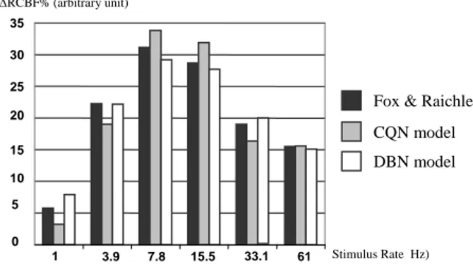
A model, adapted, in terms of a DBN, from a previous work [10], illustrates our formalism. The original model used causal qualitative networks (CQN), based on interval calculus, to explain results from two PET experiments by Fox & Raichle [1]. Their studies focused on the modulation of the activation of the striate cortex by the presentation rate of visual stimuli. The stimuli are orange square-waves pulses of constant intensity and duration (5ms) that are presented during 40s scans (PET) at rates of 1, 3.9, 7.8, 15.5, 33.1 and 61 Hz. The hypothesis is that the observed
activation is modulated by the connections between the thalamus and the cortex.
The modeled “large-scale” network is a simple anatomical loop, the cortex and the thalamus being connected by opposite oriented axon bundles. The global functional network is the connection of the two functional networks representing the striate cortex and the thalamus, plus an additional node Stim standing for the stimulus (Fig. 1). The delay for each relationship is 1 ms, excepted for the bold arrows, where it is 2 ms.
Only two magnitude functions of interest are presented here, since the task does not involve categorization processes (it uses only one type). Each input gating node (IGN) expresses the structural node’s neuronal reactivity to the stimulus. It may be considered as the abstraction, in terms of pattern and average firing rate, of the activation of the area’s pyramidal cells’ somas. For the cortex’s IGN, we have (the aX(i) being the parameters):
t IGN t IN IGN t IGN IGN t Stim t OGN IGN IGN t IGNc a c c M c M c a cM c a cM c u c M 1 1 2 2 1 3 1 -1 (3)where σIGNc is a sigmoid function used to model the zone’s
refractory period. Each Output Gating Node (OGN) sends information to the downstream areas. It represents, more or less, the integrated activity at the junction between the cells’ somas and axons. For the cortex:
t OGN t OGN OGN t IGN t FTN t IGN OGN OGN t OGNc a c c M c M c M c a cM c u c M 1 1 1 1 2 1 (4)where the sigmoid σOGNc allows using FTNc as a threshold
on IGNc. The inhibitory node INc is supposed to represent
the integrated behavior of the GABA-neurons. The firing threshold node FTNc is modulated by the thalamus, which
can lower it. Finally, the activation node ANc reflects the
level of the whole region’s blood flow variations, linked to the neuronal energy demand. It consists in the sum of the
successive IGNc’s activations during one experimental
block.
Fig. 1. The static network used to model the experiment [1].
B. Results and Comments
The time unit is 1 ms, and we used the DD1 algorithm [17] to perform the simulation. We used a sole stimulus, with a magnitude of 1 and a type made of one symbol (“orange”), repeated in order to obtain the desired stimulus rate during 40 s. The results are measures, for each 40s-scan, of the regional cerebral blood flow variations (ΔrCBF%) in the visual cortex.
Our simulation shows slightly better results than the CQN model (Fig. 2). But the real advantages are elsewhere. First, DBNs allow a better control of the dispersion of the calculated values than interval-based simulation, which
Visual Cortex Thalamic Structure Stimulus Stim IGNc INc FTNc ANc OGNt OGNc IGNt
leads, by construction [18], to a constant increase of the imprecision. Moreover, DBN can directly express nonlinear functions, which is not the case of the CQN-based simulator. Finally, a lot of algorithms for parameter estimation and inference exist and are developed for probabilistic networks. Nevertheless, the absence of precise activation data, temporally speaking, prevented us from estimating parameters using automatic methods, and forced us to define these values only by using neurological knowledge and empirical estimation.
Fig. 2. Compared results between simulated data and experimental measures.
V.CONCLUSION
Instead of building a specialized model, designed for a specific function or cerebral network, we have presented a
general framework, allowing the interpretation of
neuroimaging data concerning various tasks. This framework has been designed to be open to evolutions of the knowledge in neuropsychology and neurophysiology. The use of DBNs allowed us to model the brain as a dynamic causal probabilistic network with nonlinear relationships. We have illustrated this with an example concerning a visual perceptive process. Our future work will focus on the integration of more biological plausibility in the framework, through the representation of complex relationships between and inside the zones, and the combination of types from different categorical domains. Another essential topic is to make our models independent of the used data acquisition technique, thanks to interface models, able to translate cerebral information processing variables into neuroimaging results. Our long-term goal is to progressively include in our framework various validated generic models and to build a consistent and general brain theory based on large-scale networks.
REFERENCES
[1] P. T. Fox and M. E. Raichle, "Stimulus rate determines regional brain blood flow in striate cortex," Ann Neurol, vol. 17, pp. 303-5, 1985.
[2] G. E. Alexander, M. R. Delong, and M. D. Crutcher, "Do cortical and basal ganglionic motor area use "motor programs" to control movement?," BBS, vol. 15, pp. 656-65, 1992.
[3] P. S. Goldman-Rakic, "Topography of cognition: parallel distributed networks in primate association cortex," Annu Rev Neurosci, vol. 11, pp. 137-56, 1988.
[4] M. H. Giard, J. Lavikainen, K. Reinikainen, F. Perrin, O. Bertrand, J. Pernier, and R. Näätänen, "Separate representation of stimulus frequency, intensity and duration in auditory sensory memory: an event-related potential and dipole-model analysis," J Cogn Neurosci, vol. 7, pp. 133-143, 1995.
[5] A. N. Herbster, T. Nichols, M. B. Wiseman, M. A. Mintun, S. T. DeKosky, and J. T. Becker, "Functional connectivity in auditory-verbal short-term memory in Alzheimer's disease," Neuroimage, vol. 4, pp. 67-77, 1996. [6] C. Büchel and K. J. Friston, "Modulation of connectivity in visual pathways by attention: cortical interactions evaluated with structural equation modelling and fMRI," Cereb Cortex, vol. 7, pp. 768-78, 1997.
[7] X. J. Wang and G. Buzsaki, "Gamma oscillation by synaptic inhibition in a hippocampal interneuronal network model," J Neurosci, vol. 16, pp. 6402-13, 1996.
[8] J. D. Cohen, K. Dunbar, and J. L. McClelland, "On the control of automatic processes: a parallel distributed processing account of the Stroop effect," Psychol Rev, vol. 97, pp. 332-61, 1990.
[9] Z. Ghahramani and D. M. Wolpert, "Modular decomposition in visuomotor learning," Nature, vol. 386, pp. 392-395, 1997.
[10] J. Pastor, M. Lafon, L. Travé-Massuyès, J. F. Démonet, B. Doyon, and P. Celsis, "Information processing in large-scale cerebral networks: the causal connectivity approach," Biol Cybern, vol. 82, pp. 49-59, 2000.
[11] H. C. Leiner and A. L. Leiner, "How fibers subserve computing capabilities: similarities between brains and machines," Int Rev Neurobiol, vol. 41, pp. 535-53, 1997. [12] J. Pearl, Probabilistic reasoning in intelligent systems: networks of plausible inference: Morgan Kaufmann, 1988. [13] F. V. Jensen, An introduction to Bayesian networks. New York: Springer, 1996.
[14] T. Dean and K. Kanazawa, "Probabilistic temporal reasoning," presented at AAAI, 1988.
[15] K. Murphy, "Filtering, smoothing and the junction tree algorithm," U.C. Berkeley, Dept. Comp. Sci, Technical Report 1999.
[16] S. J. Julier and J. K. Uhlmann, "A new extension of the Kalman filter to nonlinear systems," presented at Int. Symp. Aerospace/Defense Sensing, Simul. and Controls, Orlando (FL), 1997.
[17] M. Norgaard, N. K. Poulsen, and O. Ravn, "Advances in derivative-free state estimation for nonlinear systems," Technical University of Danemark, Lyngby, Technical Repport IMM-REP-1998-15, 2000 2000.
[18] P. Struss, "Problems of Interval-Based Qualitative Reasoning," in Qualitative Reasoning: Modelling and The Generation of Behavior, H. Werther, Ed. Wien: Springer-Verlag,, 1994. Stimulus Rate Hz) 1 3.9 7.8 15.5 33.1 61 5 10 15 20 25 30 35 0
Fox & Raichle CQN model DBN model RCBF% (arbitrary unit)
![Fig. 1. The static network used to model the experiment [1].](https://thumb-eu.123doks.com/thumbv2/123doknet/2355134.37401/4.918.472.836.691.818/fig-static-network-used-model-experiment.webp)