3D Visualization of Microvascular Networks Using Magnetic Particles: Application to Magnetic Resonance Navigation

(1)

UNIVERSITÉ DE MONTRÉAL

3D VISUALIZATION OF MICROVASCULAR NETWORKS USING

MAGNETIC PARTICLES: APPLICATION TO MAGNETIC RESONANCE

NAVIGATION

NINA OLAMAEI

INSTITUT DE GÉNIE BIOMÉDICAL ÉCOLE POLYTECHNIQUE DE MONTRÉAL

THÈSE PRÉSENTÉE EN VUE DE L’OBTENTION DU DIPLÔME DE PHILOSOPHIAE DOCTOR

(GÉNIE BIOMÉDICAL) FÉVRIER 2015

(2)

UNIVERSITÉ DE MONTRÉAL

ÉCOLE POLYTECHNIQUE DE MONTRÉAL

Cette thèse intitulée :

3D VISUALIZATION OF MICROVASCULAR NETWORKS USING

MAGNETIC PARTICLES: APPLICATION TO MAGNETIC RESONANCE

NAVIGATION

présentée par : OLAMAEI Nina

en vue de l’obtention du diplôme de : Philosophiae Doctor a été dûment acceptée par le jury d’examen constitué de :

Mme PÉRIÉ-CURNIER Delphine, Doctorat, présidente

Mme CHERIET Farida, Ph. D., membre et directrice de recherche M. MARTEL Sylvain, Ph. D., membre et codirecteur de recherche M. BEAUDOIN Gilles, Ph. D., membre

(3)

DEDICATION

(4)

ACKNOWLEDGMENT

Though fascinating and unique as an experience, my route towards the end of this PhD program involved cumbersome challenges, the accomplishment of which would not be possible without the precious support of several people, to only some of whom it is possible to give particular mention here.

I would like to express my deep gratitude to my research supervisors, Professor Farida Cheriet, director of the "Imaging and 4D visualization" laboratory, and Professor Sylvain Martel, director of the "Nanorobotics laboratory". Farida has supported me throughout these years not only by providing an excellent guidance but also by furnishing my path with vision, motivation and encouragement. I am so grateful to Sylvain for his support and trust. His passion in research has undoubtedly been inspiring. His approach in dealing with compelling research problems and his high scientific standards set an example.

I would like to thank Dr. Sylvain Deschênes for his collaboration that made it possible for me to use the MRI facility at Saint-Justine hospital complemented by his insightful comments. I am also very grateful to Dr. Oleg Zabeida for his great help with the surface treatment of my microfluidic channels. He has been generous with his time and his vision. I would also like to thank Dr. Mahmood Mohammadi for his precious helps and comments on the generation of magnetic particles. I would like to thank Dr. Frederick Gosselin for his insightful discussions during the short time we worked together at Nanorobotics laboratory.

I am also indebted to the students I had the pleasure to work with. I am thankful to Azadeh Sharafi, Samira Taherkhani and Nasr Tabatabaei for being part of helpful discussions, their encouragement and empathy. I would like to thank Alexandre Bigot who was always willing to help and share his findings and experiences. Special thanks to Viviane Lalande, my French mentor and jogging partner, for her friendship and her time dedicated to correct my French writings. I am also grateful to other members of the Nanorobotics laboratory who each in one way or another helped me to complete this journey.

I would like to give a heartfelt, special thanks to my parents, Sousan and Parviz, and my dear sister, Raya, for their unconditional love and support from overseas. Without them, I would not have made it this far.

(5)

biggest supporter in this journey. He has taken care of whatever needed so that I could focus on my work. He has patiently read my thesis several times helping me to improve my writing skills. It was his constant help, encouragement and love that finally made it possible for me to see this project through to the end.

(6)

Les différentes modalités d'imagerie médicales fournissent des images cliniques de structures internes du corps humain à des fins diagnostiques et curatives. Leur première application en clinique remonte à trois décennies et depuis, grâce aux découvertes technologiques continues, de nouvelles fonctionnalités ont été intégrées aux systèmes d'imagerie. Aujourd'hui, des informations anatomiques et fonctionnelles précises peuvent être prélevées à partir de ces images dont la dimensionnalité a évolué du bidimensionnel au tridimensionnel incluant la dynamique. Une des modalités d'imagerie qui a largement profité de ces découvertes technologiques est l'imagerie par résonance magnétique (IRM). Par rapport aux autres techniques d'imagerie, l’IRM présente beaucoup d’avantages tels que la haute résolution spatiale et temporelle, le manque d'exposition aux rayonnements X et une pénétration tissulaire illimitée. Ceux-ci ont rendu l'IRM l'une des modalités les plus utilisées en clinique.

Malgré des améliorations récentes dans le fonctionnement des bobines de réception d'IRM et aussi des algorithmes de reconstruction, des progrès supplémentaires sont requis afin d’améliorer la visualisation des microstructures en clinique. La visualisation des microvaisseaux avec un diamètre de 200 µm, reste au-delà des capacités des modalités d’imageries cliniques actuelles.

Dans le traitement du cancer, une telle capacité pourrait fournir les informations nécessaires pour les nouvelles méthodes de délivrance ciblée de médicaments comme la navigation par résonance magnétique (NRM). Dans cette technique, afin d'améliorer l'indice thérapeutique, les microporteurs, chargés avec des agents thérapeutiques et des particules magnétiques, sont guidés le long d'une trajectoire qui mènerait vers une zone cancéreuse. Notre objectif est de telle trajectoire qui débuterait du bout du cathéter d'injection jusqu'à la destination finale, soit à proximité d’une zone tumorale.

Le contraste de susceptibilité magnétique dans l'IRM fournit un moyen pour prononcer l'effet d'une particule magnétique même si sa taille est beaucoup plus petite que la résolution spatiale de l'IRM. En raison de leur susceptibilité magnétique élevée, les matériaux magnétiques provoquent une inhomogénéité dans le champ magnétique local de l'IRM dans une mesure beaucoup plus importante que leur taille réelle. L’inhomogénéité apparaît dans les images de gradient écho pondéré en T2* sous forme d'une perte de signal. Cette approche présente un moyen de

(7)

simulation sur les fantômes. L’étendue de l'artefact de susceptibilité s’est avérée corrélée avec la durée d'écho, le champ magnétique statique, la taille des particules et leur magnétisation à la saturation. Selon le temps d'écho, l’étendue de l'artefact est 75 à 146 fois et de 72 à 135 fois plus grande que la taille réelle de la particule à 3,0 T et à 1,5 T, respectivement.

Des particules magnétiques d’une taille micrométrique à forte aimantation sont classées comme matériaux ferromagnétiques. En raison de la magnétisation rémanente, l'utilisation de telles particules est limitée en clinique. Comme étape suivante, l'utilisation des agglomérations micrométriques, composées de nanoparticules superparamagnétiques, en tant qu'agents de contraste en IRM a été étudiée. Les agglomérations peuvent reproduire le comportement de microparticules magnétiques en termes d’artefact de susceptibilité dans une image. Les agglomérations ont été générées en utilisant une puce microfluidique en jonction-T. Un ferrofluide à base d'huile a été utilisé pour générer les gouttelettes d’huile dans l'eau. L'avantage d'utiliser un dispositif microfluidique est le contrôle précis de la taille des gouttelettes ainsi que leur espacement. Les microagglomérations de nanoparticules d'oxyde de fer ont été injectées dans des microcanaux de 200 µm et 50 µm de diamètre interne, respectivement. Les diamètres choisis sont dans l'échelle d'une grande et une petite artériole. Les résultats ont montré que les agglomérations de 50 µm de diamètre sont juste visibles dans les images d’une séquence d’écho de gradient rapide (TrueFISP).

Par la suite, on a étudié la précision de positionnement des particules à partir de leur effet de susceptibilité sur les images. Les images reconstruites contiennent deux types d'artefacts en présence de matériaux magnétiques: la distorsion géométrique et le déplacement d'écho. La première distorsion mène à un défaut d'alignement de la position des protons tandis que la seconde distorsion provoque une perte de signal sous forme d'une "trèfle à quatre feuilles" sur les plans frontal et sagittal et un cercle sur le plan transversal. Le déplacement d'écho génère une perte de signal d’une forme symétrique dont l’origine peut représenter la position de la particule. La distorsion géométrique déplace le centre de l'artefact et peut mener à une erreur de calcul de la position de la particule. Il a été montré que le déplacement d'écho est l'effet dominant sur la distorsion géométrique dans les séquences de gradient d’écho. Alors, la position des particules a été déterminée en se basant sur leur centre de gravité. L'erreur moyenne a été calculée et elle est

(8)

des résultats.

A l'étape suivante, un réseau vasculaire 2D comprenant un canal d'entrée se diversifiant en huit canaux plus petits, en trois étapes, avec un diamètre interne de 150 µm au dernier niveau a été reconstruit. Les microagglomerations de nanoparticules d'oxyde de fer (150 ± 20 µM) ont été injectées dans un réseau vasculaire fabriqué en plexiglas en utilisant une machine de micro-usinage. Une séquence rapide multi-shot et sensible à la susceptibilité magnétique (TrueFISP) a été utilisée pour suivre les particules pendant leur injection dans le réseau. L'expérience a été répétée deux fois. La première et la deuxième expérience ont donné 70 et 114 images, respectivement. Les pertes de signal ont été identifiées visuellement et positionnées à travers leur centre de gravité. Toutes les positions ont été assemblées pour constituer la trajectoire des particules. Les résultats suggèrent que la technique peut être utilisée pour un suivi en temps réel des particules magnétiques pour regrouper les images d'un vaisseau sanguin qui est au-delà de la résolution d’un système IRM clinique.

Afin d’étendre l'approche d'une représentation 2D à 3D, nous avons proposé un nouvel algorithme basé sur la séquence TrueFISP de multi-shot et multi-tranche. La technique a été validée à l’aide d’un réseau 3D en verre. Les microagglomerations ont été injectées dans le réseau et ont été suivies dans différentes coupes. Le temps d'acquisition par coupe était de 0.6 s. L'erreur de reconstruction était plus élevée dans certains segments du réseau vasculaire. Ceci a été imposé par la limitation dans la diminution de l'épaisseur de coupe à cause de la dégradation du rapport signal sur bruit. L'erreur de mesure moyenne a été évaluée à ~ 0.4 mm.

Dans NRM, la représentation 3D des trajectoires de particules est une étape importante dans l'identification du réseau vasculaire menant au site de la tumeur. En raison de la résolution spatiale limitée des scanners d'IRM cliniques actuels, un positionnement précis des particules n’est pas possible. Cependant, le contraste de susceptibilité qui se présente dans les séquences à la base de gradient d’écho peut donner un aperçu sur la façon dont les particules sont réparties dans le champ de vision.

En conclusion, ce projet propose une nouvelle technique fiable dans la visualisation des microvaisseaux chez l’humain en utilisant un IRM clinique et les bobines réceptrices commerciales. Ceci est une étape importante dans le ciblage des tumeurs en utilisant NRM. Le

(9)

mouvement et les trajectoires mènent à une représentation 3D de la microvasculatures dans le corps humain qui n’est pas visibles à l'aide des modalités d’imageries cliniques actuelles. Les expériences in vivo restent pour valider l'application clinique de la technique proposée dans le cadre des futurs travaux. La carte 3D de la microvasculature alimentant un site tumoral mène à une amélioration significative de l'efficacité du ciblage de la tumeur en NRM tout en réduisant les effets secondaires de la chimiothérapie, le risque de reformage à la tumeur et des métastases aux autres organes.

(10)

ABSTRACT

Medical imaging modalities strive to provide clinical images of the human body’s internal structures for diagnosis and treatment purposes. Their first application in clinical trial services goes back to three decades and owing to continuous technological inventions, new capabilities have ever since been incorporated into the imaging systems. Today, anatomical and functional data with finer details and larger image sizes can be achieved and dimensionality of the images has been increased from 2D to dynamic 3D fields. One of the imaging modalities that have probably profited the most from technological findings is the magnetic resonance imaging (MRI). Compared to the other imaging techniques, MRI has various advantages such as high spatial and temporal resolution, lack of radiation exposure and unlimited tissue penetration. These have turned the MRI to one of the most available modalities clinically.

Despite recent improvements in the MRI’s receiver coils and reconstruction algorithms, further progress is yet sought to improve the visualization of the microstructures using the clinical MR scanners. Visualization of microvessels with an inner overall cross-sectional area of approximately less than 200 µm, remains beyond capabilities of the current clinical imaging modalities. In cancer therapy, such capability would provide the information required for the new delivery methods such as magnetic resonance navigation (MRN). In the MRN, to enhance the therapeutic index, microcarriers loaded with therapeutic agents and magnetic particles are navigated along a planned trajectory in the vicinity of the treatment region. Our objective is to provide such a trajectory map within an area covering the location of the catheter tip for the injection site up to the extremity of the particles’ path i.e. vicinity of the treatment region such as a tumor site.

Susceptibility-based negative contrast in the MRI provides a way to enlarge the effect of a magnetic particle whereas its actual size is much smaller than the MRI’s visualization capability. Due to their high magnetic susceptibility, magnetic materials cause an inhomogeneity in the local magnetic field of the MRI to an extent which is much larger than their actual size. The inhomogeneity appears in the T2*-weighed gradient echo images in the form of a signal void.

This approach presents a method for visualization of microstructures through the susceptibility artifact.

(11)

phantom experiments. The extent of the susceptibility artifact was found to be related to the echo time, static magnetic field, particle’s size and saturation magnetization. Depending on the echo time, the extent of the artifact is 75 to 146 times and 72 to 135 times larger than the particle’s actual size at a 3.0 T and a 1.5 T magnetic field, respectively.

Micron-sized magnetic particles with high magnetizations within the susceptibility spectrum are categorized as ferromagnetic materials. Due to the remanent magnetization, application of such particles is limited to clinical trials. As the next step, application of micron-sized agglomerations of superparamagnetic nanoparticles as contrast agents in the MRI was studied. Agglomerations can resemble the signal loss behavior of the microparticles in an image. The agglomerations were generated using a T-junction microfluidic chip. An oil-based ferrofluid was applied to generate oil in water droplets. The advantage of using a microfluidic device is the precise control over the size of the droplets as well as their spacing. Microagglomerations of iron-oxide nanoparticles were injected in microchannels of 200 µm and 50 µm in internal diameter respectively. The selected diameters are well in the scale of a large, and a small arteriole. The results showed that agglomerations of 50 µm in diameter are just visible in the images of a fast gradient echo sequence (TrueFISP).

Subsequently, the accuracy of particle positioning using their effect on the images was investigated. The reconstructed images are subject to two types of artifacts in the presence of magnetic materials: geometrical distortion and echo shifting. The former leads to a misregistration of the spins’ position while the latter causes a signal loss in the form of a four-leaf-clover on the coronal and sagittal planes and a circle on the transversal plane. The echo shifting generates symmetric signal loss shapes the centers of which can represent the origin of the artifact and thus the position of the particle. On the other hand, the geometrical distortion displaces the center of the artifact and can lead to a miscalculation of the particle’s position. It was shown that the echo shifting is the dominant effect over the geometrical distortion. Position of the particles was determined based on their center of gravity. The average error was calculated to be approximately half of a pixel’s size. The variation analysis of the results confirmed the reproducibility of the results.

(12)

channels in a three-stage division with an inner diameter of 150 µm at the last level was reconstructed. Microagglomerations of iron oxide nanoparticles (150 ± 20 µm) were injected in a vascular network made of Plexiglas using a micro-milling machine and the high-pressure thermal sealing technique. A fast multi-shot susceptibility sensitive sequence (True-FISP) was used to track the particles as they were injected in the network. The experiment was repeated twice. The first and the second trials yielded 70 and 114 images, respectively. The signal voids were identified visually and positioned through their center of gravity. All the positions were assembled to build up the trajectory of the particles. The results suggested that the technique can be used through a real-time tracking of the magnetic particles to gather images of a blood vessel which is beyond the resolution of the scanner.

In order to expand the approach from a 2D to a 3D representation of the vascular network, we proposed a new algorithm based on a fast multi-shot, multi-slice susceptibility sensitive MR sequence. The technique was validated through phantom studies in a 3D network made of glass. Microagglomerations of iron-oxide nanoparticles were injected in the network and tracked in different imaging slices. The acquisition time per slice was 0.6 s. The reconstruction error was found to be higher in some segments of the vascular network. This was realized to be due to a limitation in decreasing the slice thickness and the loss of signal to noise ratio. The mean measurement error was calculated at ~ 0.4 mm.

In MRN, 3D representation of the particles' trajectories is an important step in identification of the vascular network leading to the tumor site. Due to the limited spatial resolution of the current clinical MR scanners, a precise positioning of the particles is not possible. However, the signal loss artifact in the GRE-based sequences can shed light on how the particles are distributed within the field of view.

In conclusion, this project proposes a new and reliable technique for visualization of human microvessels using a clinical MR scanner and commercial receiver coils. This will be an important step in tumor targeting using the MRN. Real-time tracking of microagglomerations of iron oxide nanoparticles can obtain their movement trajectory. Combination of such trajectories provides a 3D representation of the microvasculatures within the human body, not visible using the current clinical imaging modalities. In-vivo experiments remain as a future work to validate

(13)

tumor site in MRN-assisted chemoembolization intervention, leads to a significant improvement on the efficiency of tumor targeting while reducing side effects of chemotherapy, risk of tumor reformation and metastases to the other organs.

(14)

LIST OF TABLES

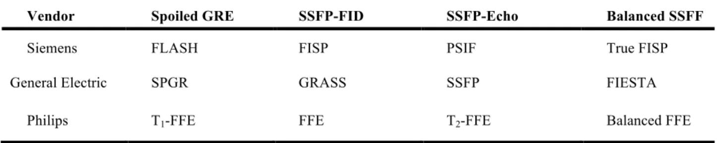
Table 2-1: Commercial names of steady state pulse sequences used by MR scanner vendors ... 28 Table 2-2: Summary of differences between imaging modalities ... 31 Table 4-1: Mean positioning errors expressed in the number of pixels (pixel size=0.5 mm) in reconstructed channels using sagittal and coronal scans. ... 52 Table 4-2: Absolute errors expressed in the number of pixels for reconstructed points from the MR scans acquired at seven different time instants. ... 58 Table 5-1: Mean measurement errors of the first and second trials ... 77

(19)

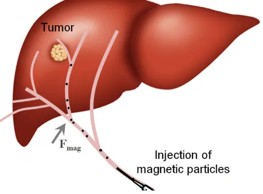
Figure 2-1: Sketch of MRI targeting of a tumor site by applying a magnetic force on volumes

loaded with therapeutic agents and magnetic particles. ... 4

Figure 2-2: A vascular network and relative vessel diameters. ... 6

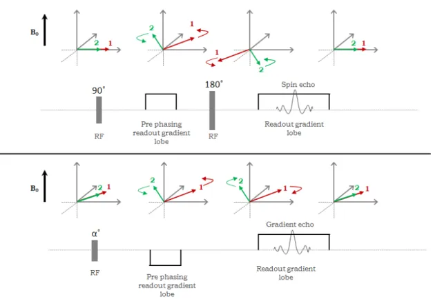
Figure 2-3: Rephasing mechanism in spin echo sequence (top) and gradient echo sequence (bottom) using RF pulses and magnetic gradients. ... 8

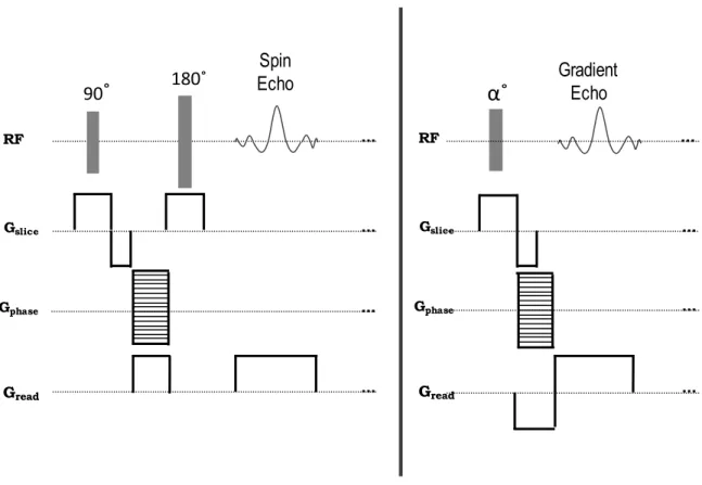
Figure 2-4: Spin echo sequence (left) versus gradient echo sequence (right). ... 9

Figure 2-5: Dispersed distribution of magnetic particles compared to clusters of magnetic particles. ... 13

Figure 2-6: Sketch of the transverse relaxivity as a function of nanoparticle’s diameter in different dephasing regimes. This curve is a representative sketch of the curve shown in Ref. [27, 43, 45]. ... 14

Figure 2-7: Effects of negative and positive background gradients during data acquisition on echo shifting in GRE-based sequences. ... 18

Figure 2-8: Presentation of magnetic field at position r!outside of a magnetic sphere with radius a. ... 19

Figure 2-9: Simulated magnetic field lines (in Tesla) (left) and the dephased volume caused by a magnetic particle (see Equations. 2-18 and 2-19) (right). ... 20

Figure 2-10: Reproduced from [60]. Comparison of voxel signals with and without geometrical distortion correction. Solid curves are numerical simulations including geometrical and intensity distortions. Dashed curves include only intensity distortion. Curve labels show image resolution in micrometers. ... 21

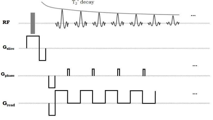
Figure 2-11: Gradient echo EPI acquisition. ... 22

Figure 2-12: Steady-state gradient echo (SSFP-FID) sequence ... 26

Figure 2-13: Balanced SSFP sequence. ... 27

Figure 2-14: Reproduced from [90]. Angiography images acquire from a 7 T MR scanner (a), which was superior to 1.5 T images (b) and comparable to DSA (c). ... 32

(20)

development acquired from a mouse embryo using a 7 T preclinical scanner. ... 33 Figure 2-16: Reproduced from [98]. In vivo high-‐resolution MRI: (a) a vasculature MIP image enhanced by 1-‐mM blood pool concentration of ferumoxtran-‐10, (b) a vasculature MIP image enhanced by 0.2-‐mM blood pool concentration of FeCo/GC, (c) picture of 2.3 cm diameter custom designed surface coil and (d) Cross-‐sectional signal intensity plot across a small vasculature. ... 34 Figure 2-17: Reproduced from [109]. Detection of single cells using a 9.4 T MR scanner at an

in-plane resolution of 23.5 µm. Slices of agarose gel containing 105 (a) and 103 (b) labeled cells. ... 36 Figure 4-1: Simulated transversal (left) and coronal (right) gradient echo images for a magnetic particle (A). Two different slices are shown in (B) Circled areas show complete signal loss which indicates the presence of a particle in each of the slices. Several slices were scanned within the volume of interest and scans were repeated for a number of times to ensure all of the particles are captured in the collected images. The third image from the top shows a complete signal loss indicating the presence of a particle in the image (C). ... 49 Figure 4-2: Images obtained from the scans at different slices. At each slice a complete signal loss indicates the presence of a particle. ... 51 Figure 4-3: Simulated 3D channel (solid line) and reconstructed points (×) using sagittal (A) and transversal (B) scans. ... 52 Figure 4-4: 2D microfluidic chip made of PMMA included a T-junction for micro-drop generation and a Y-shaped channel of 200 µm in diameter for imaging purposes (A). The T-junction was used to generate microagglomerations of nanoparticles based on the cross flowing rupture technique (B). ... 54 Figure 4-5: Emulsions of ferrofluid droplets were suspended in water in the presence of 0.1 wt% SDS to generate stabilized droplets. The average size of obtained emulsion spherical droplets was measured at 50 µm ± 20 (C) (A) Oil-based ferrofluid microagglomerations injected in a capillary tube measured 50 µm in diameter (B). ... 55

(21)

sequence (A) with the following imaging parameters: TR=500ms, TE=10 ms, slice thickness=4 mm, resolution = 256×256, pixel spacing =0.6×0.6 mm2 (A) and a TrueFISP sequence (B) with the following imaging parameters: TR=4.7ms, TE=2.6 ms, slice thickness=4 mm, resolution = 256×256, pixel spacing =0.6×0.6 mm2. ... 57 Figure 4-7: The measured points shown as * determined from the center of the artifacts (A) are compared to the real values shown as solid lines (B) to calculate the absolute measurement errors (Table 4-2). ... 59 Figure 4-8: Images of the 50 µm capillary imaged at different slices (A-D) by a 1.5 T MR scanner using a GE sequence (A) with the following imaging parameters: TR=500ms, TE=50 ms, slice thickness=4 mm, resolution = 256×256, pixel spacing =0.6×0.6 mm2_(A)

and a TrueFISP sequence (E) with the following imaging parameters: TR=5.2ms, TE=2.6 ms, slice thickness=4 mm, resolution = 256×256, pixel spacing =0.6×0.6 mm2. ... 60 Figure 4-9: The reconstructed capillary is shown by positioning signal voids in different slices shown in FIG. 4-6. At each slice the coordinates of the artifacts’ centers were calculated and collected to build a 3D distribution of the capillary. ... 60 Figure 5-1: simulated dephased volume caused by a magnetic particle (see equation 2). ... 71 Figure 5-2: (a) Schematic illustration of the T-junction, built-in reservoir and the delivery artery pattern. The dimension of the vascular network and the diameter of the branching segments are shown. (b) The effect of the surface treatment using SiO2 on the wetting property of

PMMA. ... 72 Figure 5-3: Simulated GRE signal intensity as a function of the distance between the particles on the coronal plane. The distance is labeled by multiples of the particles’ diameter (D). The curve labels represent the diameter of the particles in micrometers. The simulated coronal images of two identical iron-oxide microagglomerations with a saturation magnetization of 68 emu/gr and a diameter of 150 µm are shown. ... 74 Figure 5-4: The suspended microfluidic solution comprised of gelatin and sodium chloride with the injected microagglomerations. ... 75

(22)

network is superposed on the images by applying rigid registration to facilitate the comparison. ... 77 Figure 5-6: The measured points from the first (×) and second (o) trials superposed on the vascular network’s pattern. (b) The acquired data at each segment were fit based on a first-degree polynomial equation and the estimated vascular network was obtained. ... 78 Figure 6-1: Clinical MRI (left) and microscopic (right) images of a capillary with an inner diameter of 50 µm injected by agglomerations of Magnetite particles. ... 95 Figure 6-2: Random distribution of the magnetic particles (circles) on the vascular network (dotted lines) and their intersection with a coronal slice (A), form of the artifacts on the corresponding slice as they appear in MR images of a GRE sequence (B). Reconstructed points (×) and the simulated vascular network using coronal slices (C). ... 96 Figure 6-3: Diagram of the steps performed in the simulation of a multi-slice, multi-acquisition MR imaging of a vascular network. ... 97 Figure 6-4: Experiments setup; suspended vascular network in a container filled with water and Sodium Chloride. The continuous phase (water, Glycerol and SDS) and ferrofluid are injected through the T-junction prior to the network’s inlet. ... 98 Figure 6-5: Susceptibility artifacts within multiple coronal slices at different time instants with the following imaging parameters: imaging matrix= 256×256, pixel spacing= 0.7813×0.7813 mm2, TR = 4.32 ms, TE = 2.16 ms, slice thickness = 3.6 mm, and flip angle = 70˚ (A). Complete signal losses (circled artifacts) were considered to resemble the presence of a particle within the imaging slice (B). ... 99 Figure 6-6: 3D reconstructed points (●) through the localization of the micro-agglomerations of Magnetite particles at 16 different acquisitions and 17 different slices. The points at each segment were fitted (solid line) based on a polynomial regression model in three dimensions (A). The measured points (●) superposed over the 3D reference image obtained from a 3D scan with the following parameters: Imaging volume = 256×512×128, pixel spacing = 0.39×0.39×0.80 mm3, TR = 22 ms, TE = 9.2 ms and flip angle = 30˚ (B). ... 100

(23)

relation to the imaging coronal planes (A). Mean measurement error and the standard deviation for each segment based on coronal planes data (B). ... 101 Figure 6-8: Combined imaging planes and 3D coordinates extracted from coronal and transversal imaging planes. ... 102 Figure 6-9: The coronal data (black) and the combined coronal-transversal data (gray) were fitted at each segment based on a polynomial regression model in three dimensions (A). Mean measurement error and the standard deviation for each segment based on the combined coronal-transversal data (B). ... 103 Figure 7-1: The design of the vascular in the CircuitCAM software. ... 104 Figure 7-2: The final milled PMMA sealed in the press machine. ... 105 Figure 7-3: Formation of undefined oil droplets in water in a T-junction geometry with hydrophilic channels. ... 106 Figure 7-4: Impact of silica coated PMMA on the wetting property of the surface. ... 107 Figure 7-5: A milled PMMA and its mask to exclusively expose channels to the Silica treatment.

... 108 Figure 7-6: A milled PMMA with exposed channels’ surface prior to Silica coating. ... 109

(24)

LIST OF SYMBOLS AND ABBREVIATIONS

2D Two dimensional

3D Three dimensional

BOLD Blood oxygenation level independent

b-SSFP Balanced steady state free precession

COG Center of gravity

CT Computerized tomography

CTA Computerized tomography angiography

DCE Dynamic contrast enhanced

DSA Digital subtraction angiography

EPI Echo planar imaging

FISP Fast imaging with steady state precession

fMRI Functional magnetic resonance imaging

FOV Field of view

FT Fourier transform

GRE Gradient Recalled echo

MAR Motional averaging regime

MION Monocrystaline iron oxide nanoparticles

MNP Magnetic nanoparticle

MPIO Micron-sized iron oxide

MR Magnetic resonance

MRA Magnetic resonance angiography

(25)

MRN Magnetic resonance navigation

MVD Microvessel density

NMR Nuclear magnetic resonance

OCA Optical coherence angiography

OFDI Optical frequency domain imaging

PCB Printed circuit board

PMMA Polymethylmethacrylate

RES Reticuloendothelial system

RF Radio frequency

ROI Region of interest

RTM Residual transverse magnetization

SDR Static dephasing regime

SDS Sodium Dodecyl Sulfate

SE Spin echo

SENSE Sensitivity encoding

SMASH Simultaneous acquisition of spatial harmonics

SNR Signal to noise ratio

SPIO Superparamagnetic iron oxide

TE Echo time

TMMC Therapeutic magnetic micro carriers

TR Repetition time

USPIO Ultra small Superparamagnetic iron oxide

(26)

LIST OF APPENDICES

appendix A – Visibility of magnetic microparicles in clinical MR images ... 132 appendix B –Positioning of magnetic microparticles using susceptibility artifacts ... 137

(27)

CHAPTER 1 INTRODUCTION

Cancer is a major chronic disease and a leading cause of mortality in Canada and around the world. Depending on type, number, location and stage of the cancerous tumors, one treatment option or a combination of different type of treatments may be considered. Palliative treatments prevent or slow the development of the cancer cells. In contrast, curative treatments seek to achieve a complete removal of cancer cells.

Surgery is a conventional therapeutic choice for localized and small cancer tumors. It is a curative approach to achieve a complete tumor resection or replacement [1]. It can be used alone or along with a complementary method such as chemotherapy or radiation therapy [2]. It can also be complemented by radiation therapy during the operation.

Radiation therapy uses high-energy radiations such as X-ray, gamma ray or protons to kill cancer cells through damaging their DNA. It can be performed locally or systematically and can be used before or after surgery to enhance or complete the main treatment. Due to the limitation on the radiation dose, this palliative technique is usually performed as a complementary treatment [3, 4].

Chemotherapy is a systemic palliative treatment that uses medicines to kill cancer cells. Medication can be received orally, intravenously or intra-arterially. During chemotherapy, drugs travel throughout the whole body to reach cancer cells. However, healthy cells are inevitably damaged as well. Chemotherapy is often prescribed as a complementary treatment after the surgery or radiation therapy to kill the remaining cancer cells or before the main treatment to shrink the tumors [5, 6].

Chemoembolization is a combination of chemotherapy and embolization procedure mostly used in the liver treatment. In this method drugs are intra arterially injected into the blood vessel supplying the tumor. Subsequently, embolic agents are released to embolize the vessel’s entry and trap the drugs in the tumor by ceasing the blood supply [7, 8]. Accordingly, a highly concentrated dose of therapeutic agents are delivered to the tumor site and the feeding blood vessels are partially occluded to starve the tumor of nutrients.

Targeted therapy is a fairly new type of treatment developed to attack cancer cells with reduced harm to the healthy tissue. In this technique drugs or other substances are applied that interfere

(28)

therapies are based on interactions with mediators capable of ceasing the development of cancerous tissue. Depending on the type of cancer, targeted therapy can be achieved through interference with the development of angiogenesis, prevention of cell growth signaling, stimulation of the immune system to destroy cancer cells or specific delivery of therapeutic agents to the cancer cells [9-11].

Magnetic resonance navigation (MRN) assisted chemoembolization has been proposed to overcome the drawbacks of older interventions. It has shown a great potential in targeted delivery of magnetic carriers loaded with therapeutic agents [12, 13]. The technique is based on therapeutic magnetic micro carriers (TMMC) which can be steered and tracked using an upgraded magnetic resonance imaging (MRI) system.

TMMC consists of biodegradable microparticles encapsulating magnetic nanoparticles and the antitumor drug. They measure 50 µm in diameter. The external magnetic field of the MRI (B0)

magnetizes the microparticles to saturation. The catheter tip can only be advanced to the level of the arteries. However, the tumor is located at the capillary level. Upon the release of the TMMCs, custom gradient coils are applied to induce a directional propulsion force on nanoparticles, embedded in the micro carriers. This technique leads to the controlled delivery of the therapeutic agents to the region of interest. In vivo targeting of the right or left liver lobes has been successfully achieved by MRN through the hepatic artery in a rabbit model [12]. The steering has been performed through a single bifurcation. However, steering through multiple bifurcations necessitates a precise map of the vasculature leading to the tumor. The gradient coils are applied according to a 3D pre-planned map of the local vasculature feeding the cancer tumor. Consequently, preparation of such a map is an essential step in this intervention. Current clinical imaging modalities are limited in resolving the vasculatures smaller than approximately 200 µm in diameter. As such, the visualization of arterioles and capillaries remain beyond the capability of current clinical imaging modalities.

This research study seeks to develop a clinical imaging technique to identify the vascular path leading to a tumor site with the purpose of improving the MRN technique. The development of such a map leads to steer the TMMCs through multiple bifurcations in the vascular network, enhancing the steering efficiency and reducing the side effects of the anti-cancer medications.

(29)

chapters. Chapter 2 presents a background on MR imaging and a relevant literature review on microvascular imaging. Chapter 3 discusses the assumptions and objectives of the thesis and the overall approach adopted to accomplish each objective. Chapters 4, 5 and 6 are devoted to original contributions of this thesis, corresponding to three articles published or submitted to peer-review journals. Chapter 4 includes the article accepted in March 2013 to be published in the «Journal of Applied Physics». It represents the visualization of microchannels measuring 50 µm in diameter, corresponding to small arterioles, using superparamagnetic iron oxide nanoparticles and a clinical MR scanner. Chapter 5 includes the article accepted in May 2014 for publication in the journal of «Applied Physics Letters» and it represents dynamic tracking of magnetic nanoparticles clusters for mapping microvascular networks. Chapter 6 includes an article on proposing and validating a method for 3D mapping of vascular network through a fast multi-slice multi-acquisition MR sequence. The article was submitted in October 2014 to the Journal of «IEEE Transactions on Biomedical Engineering». Chapter 7 presents a new technique developed for fabrication of an integrated microfluidic device to generate and inject iron oxide microagglomerations in a vascular network. Chapter 8 provides a discussion on all the work carried out during this research study. Finally, the conclusion discusses the contributions of this thesis and new avenues of research and recommendations for future works are also proposed.

(30)

CHAPTER 2 LITERATURE REVIEW

2.1 Magnetic resonance navigation (MRN)

Navigation of an untethered device in a living subject is of great interest for both therapeutic and diagnostic purposes. MRN is a newly developed approach to navigate an untethered micro device to a targeted location within the body accessible through the vascular network [14, 15]. The extremity of the catheter injecting therapeutic agents can only be advanced to the arterial level whereas tumors are often located at the capillary level (figure 2-1).

Figure 2-1: Sketch of MRI targeting of a tumor site by applying a magnetic force on volumes loaded with therapeutic agents and magnetic particles.

Therefore, a significant portion of the injected drug reaches the systemic circulation. In MRN, micro carriers loaded with therapeutic agents and magnetic particles are released and subsequently steering gradients are applied to navigate the carriers towards a selected capillary entry where the tumor is located (figure 2-2).

(31)

In [16], propulsion of a magnetic core in the carotid artery of a living swine showed feasibility of the technique in-vivo. Three orthogonal gradient coils inside a magnetic resonance imaging (MRI) scanner can induce a three dimensional directional magnetic force on a magnetic object. The magnetic force (Fmag) is proportional to the amplitude of the gradient vector and the magnetic moment of the object according to:

(

M

)

B

RV

F

!

_mag

=

⋅

∇

(Eq. 2-1)

where R is the duty cycle of the gradient, V and

M

!

are the volume and the magnetization of the magnetic object, respectively,

B

!

is the magnetic field and ∇the vector differential operator.

In order to propel a magnetic object in the vascular network, the magnetic force should surmount the drag force applied by the flow. The weight of the magnetic object and its buoyancy can be neglected in small blood vessels since such parameters are smaller than the drag force by several orders of magnitude. Therefore, to achieve a strong magnetic force, magnetization of the magnetic object and the magnetic field gradient generated by the gradient coils should be maximized. In [17], a proportional-integral-derivative controller was used to navigate a ferromagnetic core along a predefined trajectory in real time. Operating inside an MRI system prevents simultaneous application of propulsion and tracking using MR images. Real-time tracking necessitated an alternation between these two processes. An advanced MR sequence based on magnetic signature selective excitation was developed and employed for fast tracking of a single magnetic object [18, 19].

Clinical MRI systems are typically capable of providing tens of mT/m of gradient in any direction. Such gradients are potentially capable of providing enough force to propel a ferromagnetic core, saturated in the magnetic field of an MRI, with a diameter of ~0.6 mm [14]. However, gradient amplitudes of several T/m would be required to propel a smaller ferromagnetic core or in smaller vascular networks. Compared to their ferromagnetic counterparts, superparamagnetic particles that are vastly used as contrast agents in MRI hold a significantly smaller magnetization. However, an agglomeration of such nanoparticles can be used as a steerable magnetic volume for therapeutic purposes. Their relative low magnetization should be compensated by application of higher gradient amplitudes.

(32)

In [13], therapeutic magnetic micro carriers (TMMC) were guided in real time in a phantom including a single bifurcation using magnetic gradients of 400 mT/m. TMMC were biodegradable microparticles loaded with iron cobalt nanoparticles. These particles possess a high saturation magnetization (72 emu/g) and therefore are an excellent candidate for both imaging and navigation purposes. Subsequently, TMMC particles loaded with doxorubicin were steered in-vivo to the left liver lobes through one bifurcation in a rabbit model using a clinical MR scanner equipped with upgraded gradient coils of 400 mT/m [12, 20]. Results suggested the potential of MRN for improving drug targeting in deep tissues.

In-vivo and in-vitro experiments have been performed to confirm the effectiveness of MRN in targeted drug delivery. Thus far, navigation of micro carriers has been carried out in-vivo through a single bifurcation and in-vitro inside a three bifurcation PMMA phantom [21]. However, the ultimate goal in MRN is to navigate microcarriers in-vivo through a vascular network of multiple bifurcation levels to the entry of a selected capillary. The direction and the time at which the magnetic gradients are applied depend on the local vasculature’s map feeding the tumor. As such, preparation of a 3D map of the microvasculature prior to the intervention is a crucial step in MRN.

(33)

Current clinical angiography modalities can help to provide such a map. In section 2.3, the visualization of the vascular network using current clinical imaging modalities will be discussed.

2.2 Magnetic resonance imaging

MRI uses strong magnetic field and radio frequency waves to generate cross sectional images of internal structures of the body. This technique has profited from technological innovations to improve quality of the images as well as the acquisition speed. Subjected to a large magnetic field (B0), Hydrogen atoms (protons) become aligned with the direction of the field. By applying

a properly tuned radio frequency, protons will be tipped out of alignment with B0. Upon removal

of the radio wave, the protons tend to return to their equilibrium state in a process called relaxation. The relaxation causes variations in transverse magnetization vector that causes a small alteration in the induced electrical current in the receiver coil. The signal is quite sensitive to differences in proton content which is a distinctive characteristic of different types of tissue.

Each MR sequence is a combination of magnetic gradients and radio frequency waves. Frequency encoding gradient encodes nuclear magnetic resonance (NMR) signal spatially by assigning a unique frequency to the spins at different locations along its direction. Therefore, the time-varying NMR signal consists of a range of frequencies, each corresponding to a particular spatial location. The range of frequency precession (Δω) along the x-direction (Δx) where Gx is applied can be calculated according to:

x G_xΔ = Δ

π

γ

ω

2 (Eq. 2-2)

where γ is the gyromagnetic ratio of the protons (42.56 MHz/T). A Fourier transform of the NMR signal reveals the density of spins at each frequency. A frequency-encoding gradient can be applied along any physical direction. It consists of two lobes; prephasing (or dephasing) lobe and readout (or rephasing) lobe. The prephasing lobe prepares the transverse magnetization so that an echo can be formed later in time. In spin echo (SE) sequences, the two lobes are separated by a 180˚ refocusing pulse. Since the refocusing pulse inverses the accumulated phase during the prephasing lobe, the readout lobe has the same polarity as the prephasing lobe (in order that the spins continue to accumulate phase in the same direction).

(34)

Due to the absence of a 180˚ refocusing pulse, in gradient echo (GRE) sequences the readout lobe is reversed to change the direction of the spin’s phase accumulation. The gradient reversal refocuses only the spins dephased by the action of the pre-phasing gradient lobe. Therefore, as opposed to a SE, phase dispersions resulting from magnetic field inhomogeneities, chemical shifts or susceptibility gradients are not cancelled at the center of the GRE (figure 2-3). The time between the application of the radio frequency (RF) excitation pulse and the peak of the echo signal is known as echo time (TE). The time between the successive excitation pulses is known as repetition time (TR).

Figure 2-3: Rephasing mechanism in spin echo sequence (top) and gradient echo sequence (bottom) using RF pulses and magnetic gradients.

Peak of the gradient echo occurs when the area under the two opposing lobes is equal. Consequently, GRE images are weighted by a factor of exp −TE T2

*

(

)

versus exp −TE T

(

2

)

in SE

(35)

1 T

*₂

=

1 T

₂

+

1 !

T

₂ (Eq. 2-3)

where T´2 is inversely proportional to the magnetic field inhomogeneity in each image voxel.

In-plane spatial localization necessitates the employment of both frequency and phase encoding gradients. Phase encoding gradient is typically applied orthogonal to the frequency encoding direction. It is applied when the magnetization is in the transverse plane and prior to the application of the readout gradient. The area under the phase encoding gradient varies at each TR to introduce different amount of phase variations to the spins along its direction.

In order to achieve a desired spatial location in a 3D volume, slice selection gradients are applied concurrently with the RF pulses. The slice selection gradient determines the direction perpendicular to the imaging plane (figure 2-4).

Figure 2-4: Spin echo sequence (left) versus gradient echo sequence (right).

GRE sequences can be fast as no refocusing pulse is present and subsequently no long-lasting T1 recovery time is required.

RF Gslice Gphase Gread 90

˚

180˚

α˚

Spin

Echo Gradient _Echo

RF

Gslice

Gphase

(36)

2.2.1 Magnetic particles in MRI

Magnetic nanoparticles have been widely investigated in biomedical applications such as hyperthermia, targeted drug delivery and contrast agents in MRI and dual-modality imaging [22-27]. MRI provides an excellent soft tissue contrast whereas its inherent low sensitivity does not convene the visualization of the microstructures. To enhance its sensitivity, contrast agents are applied. Contrast agents are categorized into a) gadolinium-based paramagnetic agents and b) superparamagnetic nanoparticles. Due to a lower magnetization saturation, gadolinium-based contrast agents have a lower sensitivity compared to that of their superparamagnetic counterparts [28]. Free gadolinium ions have a toxic effect that can be nephritic [29, 30]. Iron oxide nanoparticles have shown a superior biocompatibility and biodegradability [31]. Injected iron oxide nanoparticles are cleared through the macrophage process in the reticuloendothelial system and subsequently degraded in the lysosomes.

2.2.1.1 Paramagnetism versus superparamagnetism

Paramagnetism is the characteristic of the atoms or ions with an unpaired number of electrons in their outer shell. As such, these individual atoms or ions possess intrinsic magnetic dipole moments. However, due to the random orientation of the individual magnetic dipole moments, an agglomeration of them does not reveal any magnetization property. Once subjected to an external magnetic field, individual atoms orient along the direction of the magnetic field. Upon removal of the applied magnetic field, all the individual atoms return to their original orientation. Due to thermal agitation, not all the individual paramagnetic atoms can be aligned with the magnetic field unless they are subjected to temperatures of near absolute zero (-273˚C). Gadolinium (Gd3+) is one of the strongest paramagnetic substances widely used as MR contrast agents.

Unlike paramagnetism which is the property of the individual atoms and ions, ferromagnetism is the property of a group of atoms, ions or molecules in a solid crystal. Ferromagnetic materials possess multiple domains with random orientations due to which they do not show any magnetization property. Once subjected to an external magnetic field, all the individual domains orient parallel to the direction of the magnetic field. As opposed to paramagnetic materials, ferromagnetic materials can become fully magnetized at practically obtainable field strengths and room temperatures. Upon removal of the magnetic field, the individual domains maintain their

(37)

orientation parallel to the magnetic field. This effect is due to the fact that parallel alignment is a preferred low-energy state and thus some energy is required to demagnetize the ferromagnetic materials. It is possible to obtain a single magnetic domain particle by decreasing size of the multi-domain particles to approximately that of the nanometer sized agents. These single-domain nanoparticles are called superparamagnetics having unique magnetic properties. Similar to the ferromagnetic particles, they can become magnetized to saturation even at a low magnetic field and like the paramagnetic particles they will not retain any net magnetization property in the absence of an external magnetic field. The size of the individual magnetic domains depends on the magnetic anisotropy and is in the order of tens of nanometers. A transition from multi domain structure to single domain structure occurs with the reduction of the particles size to ~ 40 nm. This transition is accompanied by a significant reduction in the saturation magnetization [32].

2.2.1.2 Superparamagnetic iron oxide nanoparticles

Superparamagnetic iron oxide (SPIO) contrast agents are based on water insoluble iron oxide crystals of Fe3O4 (magnetite) or γ-Fe2O3 (maghemite) with a core diameter in the range of 4 - 12

nm. However, the overall diameter of these particles is considerably larger than their core size (5 nm - 1µm). The iron oxide particles are coated with an organic polymer to prevent their aggregation [33, 34]. The principal effect of the SPIOs is on the T2* relaxation time. MR imaging

of such nanoparticles is usually performed using the T2*/T2-weighted imaging sequences. The T1

relaxation time is also affected by the SPIOs enabling the T1-weighted imaging with a less

pronounced positive T1- contrast [35]. Depending on the distribution of the particles’ size and

their overall diameter, iron oxide contrast agents are divided into three groups; a) standard SPIO agents, ultra small SPIOs (USPIO) and monocrystalline iron oxide nanoparticles (MION). Several parameters, such as size and coating and concentration of the particles within an imaging voxel, affect the relaxometric behavior of the SPIOs.

Standard SPIOs have a high T2/T1 relativity ratio and their overall size varies in the range of 60

-150 nm. They are composed of agglomerated iron oxide cores and in the presence of a magnetic field can get separated from the solution. Intravenously injected SPIOs are easily sequestered by the reticuloendothelial system (RES) cells in the liver, spleen and bone marrow (half-life, 3 days) [36].

(38)

The USPIOs have a smaller hydrodynamic diameter (10 – 50 nm) and a longer half-life. Owing to their small size, Brownian motion keeps them suspended in water in spite of their higher density. These agents can cross the capillary wall and spread to the tissue. Due to their long blood half-life, they can be used as blood pool contrast agents in the MR angiography [37, 38].

The MIONs are very small in size (2 – 9 nm) and are usually used for receptor-directed and magnetically labeled cell probe MR imaging [39, 40]. Their core contains one central Iron oxide particle only and due to their small size they easily pass through the capillary endothelium.

Contrast agents are used to enhance the sensitivity of the MRI through shortening the T1 and

T2 relaxation times. The efficiency of a contrast agent is evaluated by the relaxivity (r1, r2 and r2*,

inverse T1, T2 and T2* respectively). R2* relaxivity indicates an increase in the T2 relaxation time

in the GRE sequences due to a magnetic inhomogeneity called the susceptibility effect:

R2 *

= R2+γBs (Eq. 2-4)

where γBs represents the relaxation induced by the magnetic inhomogeneity. The term susceptibility effect describes an increase in the T2/T2* relaxation rates due to a difference in

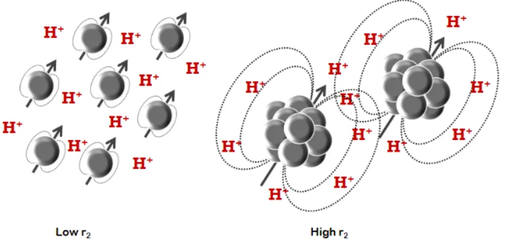
magnetization within a voxel. Non-homogeneous distribution of magnetic particles induces a local field gradient which causes the spins to lose coherence at an accelerating rate. The susceptibility-induced relaxation can affect the protons located much farther from the magnetic cores. On the other hand, a homogeneous or dispersed distribution of the magnetic particles results in another contrast mechanism where because of a free water access to the contrast agent sites, the proton relaxation is due to an interaction between each of the individual magnetic particles and water molecules (figure 2-5).

Two SPIO-based contrast agents are clinically approved: ferumoxides (Feridex in the USA, Endorem in Europe, diameter of 120 to 180 nm) and ferucarbotran (Resovist, diameter of 60 nm).

2.2.1.3 Clusters of magnetic nanoparticles

An assembly of magnetic nanoparticles can be used to further enhance the contrast. Agglomerations of magnetic nanoparticles significantly affect the transverse magnetization [27]. It was shown that the sensitivity of MRI is comparable to the one of PET in detecting single cells using an assembly of SPIO nanoparticles [41].

(39)

Figure 2-5: Dispersed distribution of magnetic particles compared to clusters of magnetic particles.

The R2 relaxivity rate increases with the agglomeration’s size, reaches a maximum and

decreases subsequently. On the other hand, the r1 relaxivity is only slightly affected by the size of

the agglomerations [42-45]. Compared to the large agglomerations of the magnetic nanoparticles, free magnetic particles show a different contrast mechanism. Since diffusion of the magnetic particles is dependent on their size, different mechanisms can be defined based on the translation diffusion time around the nanoparticles agglomerations. The diffusion time is defined as:

τD =

r2

D (Eq. 2-5)

where r is the radius of the nanoparticles or the agglomerations, and D is the diffusion coefficient of the water molecules. The diffusion time is the time for a water molecule to pass a hemisphere of a nanoparticle or an agglomeration.

There are two spin dephasing regimes: the motional averaging regime (MAR) where the water diffusion is the main factor in spin dephasing and the static dephasing regime (SDR) where the relaxation rate is independent of diffusion. For short diffusion times (τ_D <<1Δw_r where Δwr is

the difference in the angular frequency experienced by a proton between the local fields) the particles are homogeneously dispersed in the solution. In MAR, the diffusion time is much smaller than the echo time and no difference is observed between the r2 and r2* relaxation rates

(40)

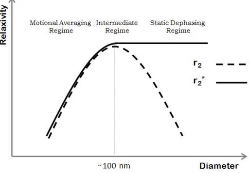
In SDR, whereτD> 1 Δwr , randomly distributed large agglomerations create an inhomogeneous magnetic field. If the particles or the size of the agglomerations are large enough, compared to the inter-particle distance, the diffusion of water is small and as such, it can be ignored. In this regime, r2 decreases with particles’ size and r2* reaches a constant value (figure

2-6) [43, 47]. The r2 relaxivity tends to decrease in SDR regime due to the fact that the RF

refocusing pulse becomes effective in rephasing the spins. Trend of the r2/ r2* relaxivity changes

according to the regime where the particles are in.

Figure 2-6: Sketch of the transverse relaxivity as a function of nanoparticle’s diameter in different dephasing regimes. This curve is a representative sketch of the curve shown in Ref. [27,

43, 45].

Beyond the SDR, the induced magnetic field created by the magnetic particles is so strong that the adjacent protons are completely dephased. Accordingly, the surrounding water protons do not contribute to the MR signal [27]. Nanoparticle clusters and spherical-shaped particles demonstrate the same relaxivity behavior as their size varies. It was shown that nanoparticle cluster size was linearly related to the r2 of clusters in the MAR [44], and inversely related to the

(41)

2.2.2 Susceptibility contrast in MR images

In this section, the susceptibility effect in MR images with a focus on the presence of magnetic particles in the region of interest is explained. According to the imaging sequence two types of artifacts (geometrical and intensity distortion) can occur in the images that are explained in details.

2.2.2.1 Susceptibility

A one to one relationship between a spin’s position and the frequency at which it precesses is the basis of the spatial encoding in the MRI. An inhomogeneity in B0 causes a variation in the

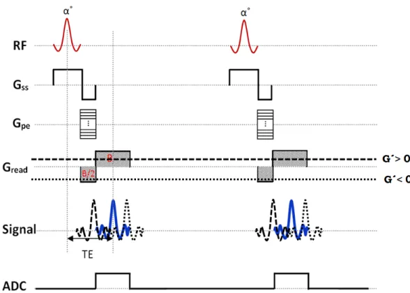
precession frequency creating susceptibility artifacts in the MR images. Magnetic susceptibility is a dimensionless quantitative measure of the level of a material’s ability to induce a local magnetic field inhomogeneity within an applied homogeneous magnetic field. Macroscopic field inhomogeneities give rise to two types of artifacts: geometrical distortion and intensity distortion (echo shifting). The first artifact causes a misregistration of the spin’s location in the form of a shift in spins’ position or a "shearing" effect on the image, depending on whether the background gradient is parallel or perpendicular to the read-out direction. The second artifact only affects the gradient echo imaging.

2.2.2.1.1 Geometrical distortion

If a background gradient (G´x), parallel to the read-out gradient’s (Gx) direction, is present during the echo acquisition, the phase evolution of the spins alters [49]:

( )

t

'

₌

₋

2 _πγ

(

G

_x

x

₊

G

'

_x

x

)

t

'

φ

(Eq. 2-6)

( )

'

2 '

1 '

t

'

G

x

t

G

t

x x x

_⎟⎟

⎠

⎞

⎜⎜

⎝

⎛

+

−

=

πγ

φ

(Eq. 2-7)

It is assumed that the read-out gradient is applied along the x-direction. As such, the spins residing at position x will be mapped to an apparent position x´ and the reconstructed spin density spatially differs from the physical spin density:

⎟⎟ ⎠ ⎞ ⎜⎜ ⎝ ⎛ + = x x G G x x' 1 ' (Eq. 2-8)

(42)

The presence of the G´x causes the spins to be shifted parallel to the read-out direction. Increasing the applied read-out gradient is the only way to minimize the distortion. If G´x is known throughout the FOV, the distortion can be corrected through shimming.

Any background gradient during data recording will change the frequency at which the spins precess and lead to a misregistration of the spins’ location. If G´ is perpendicular to the read-out direction (G´y orG´z), the spins will be shifted along the x-direction as a function of their position in the z or y-direction. If the background gradient is in the y-direction, the phase behavior during the read-out varies as following:

( )

t

'

=

−

2 πγ

(

G

_x

x

+

G

'

_y

y

)

t

'

φ

(Eq. 2-9)

( )

' 2 ' y t' G G x G t x y x _⎟⎟ ⎠ ⎞ ⎜⎜ ⎝ ⎛ + − =

πγ

φ

(Eq. 2-10) y G G x x x y ' '= + (Eq. 2-11)

This effect distorts the square shape of the voxel and as a result the reconstructed voxels contain information from the adjacent spatial locations.

2.2.2.1.2 Intensity distortion

Due to the absence of the 180˚ refocusing pulse, intensity distortion pertains to the gradient echo sequences. In 2D Fourier transform (FT) the MR signal is given by [50, 51]:

(

)

(

)

( )

∫ ∫ ∫

∞ ∞ − ∞ ∞ − ∞ ∞ −

=

M

x

y

z

e

dxdydz

m

n

s

_,

iφ x,y,z,n.m (Eq. 2-12)

where n and m represent number of the time sample and that of the phase encoding step, respectively, and M represents the distribution of the magnetization right after the application of the RF excitation pulse.

In the absence of a background gradient with slice selection along z, phase encoding along y and frequency encoding along the x direction, phase evolution during the sampling period is given by [50, 51]:

3D Visualization of Microvascular Networks Using Magnetic Particles: Application to Magnetic Resonance Navigation