Flow forcing techniques for numerical simulation of combustion instabilities

(1)

HAL Id: hal-00910199

https://hal.archives-ouvertes.fr/hal-00910199

Submitted on 29 Nov 2013

HAL is a multi-disciplinary open access archive for the deposit and dissemination of sci-entific research documents, whether they are pub-lished or not. The documents may come from teaching and research institutions in France or

L’archive ouverte pluridisciplinaire HAL, est destinée au dépôt et à la diffusion de documents scientifiques de niveau recherche, publiés ou non, émanant des établissements d’enseignement et de recherche français ou étrangers, des laboratoires

Flow forcing techniques for numerical simulation of

combustion instabilities

André Kaufmann, Franck Nicoud, Thierry Poinsot

To cite this version:

André Kaufmann, Franck Nicoud, Thierry Poinsot. Flow forcing techniques for numerical simulation of combustion instabilities. Combustion and Flame, Elsevier, 2002, 131 (4), pp.371-385. �10.1016/S0010-2180(02)00419-4�. �hal-00910199�

(2)

Flow forcing techniques for numerical simulation of

combustion instabilities

A. Kaufmann, F. Nicoud

∗

CERFACS, Toulouse, France

T. Poinsot, IMF Toulouse, UMR5502, Toulouse France

June 20, 2002

Corresponding author: A. Kaufmann (kaufmann@cerfacs.fr) CERFACS

42 Av. Coriolis

31057 Toulouse, France

(3)

Abstract

Investigation of combustion instabilities in gas turbine combustors require the knowledge of flame transfer functions. Those can be obtained by experimental mea-surement or by Large Eddy Simulations (LES). Since calculations are usually limited to a portion of the whole combustor, boundary conditions are of crucial importance. It is common practice to inject acoustic perturbations for the flame transfer function measurement in form of velocity perturbations (u′_{(t)). We present an alternative}

method based on a characteristic treatment of the Euler Equations [1], [2]. It con-sists of injecting sound waves travelling into the computational inlet while letting outgoing waves leave the domain without reflection. This method has several advan-tages concerning the study of flame transfer functions compared to injecting velocity perturbations. Both techniques are compared for cases where analytical solutions may be derived ( a duct without flame and a planar laminar flame ) and for one case where a CFD code is necessary ( a laminar Bunsen-type flame [3]).

(4)

1 Introduction

Pollutant formation in gas turbines has become an important issue for gas turbine con-structors. Several methodologies are being designed and tested by constructors in order to match the emission levels set by international agreements. Lean premixed prevapor-ized (LPP) combustors have better pollutant properties concerning N Ox formation but

are more sensitive to combustion instabilities [4], [5]. Acoustic waves in the combustor perturb heat release by generating fluctuations in mixture fraction and/or flame surface [6], [7], [8]. If this unsteady heat release couples with acoustics, some eigenfrequencies of the combustor may be encouraged depending on the time lag between acoustic waves and unsteady combustion. Understanding and preventing the resulting resonances are key issues in the present development of many LPP combustion chambers.

Linear acoustics (see for instance [9], [2], [10], [11] ) may be used to analyse, model acoustic-combustion interactions and predict self sustained frequencies in gas turbine com-bustors. In these studies the flame is viewed as an acoustic device which generates an unsteady heat release depending on the local acoustics. Simple interaction models usually consist of a frequency dependent transfer function, relating heat release fluctuations with pressure and/or velocity fluctuations. Transfer functions depend not only on frequency,

(5)

but also on the geometry, the operation mode of a given combustor, and more generally on the interaction of vortices induced by acoustic waves with the flame front. Thus, even though transfer functions may in simplified configurations be derived from an analytical analysis, attempts to use such analytical models in complex combustion chambers have had mitigate success (see [12]). As a result, costly non trivial experiments are often required in order to gain some insight about the flame response to acoustic fluctuations. An alterna-tive method to obtain transfer function has turned up with Large Eddy Simulations (LES) ([2], [13], [14], [15], [16]). These calculations have the potential to provide quantitative data about the flame response. The following requirements must be matched by the LES tool in order to obtain reliable information for flame transfer functions in gas turbines :

1. the full three dimensional compressible Navier Stokes equations must be solved on unstructured meshes for complex geometries [17],

2. numerical methods with small dissipation/dispersion [18], compatible with LES method-ology have to be used,

3. LES model for flow dynamics in complex wall bounded flows [19] are required,

4. the LES chemistry/turbulence interaction model must be valid for premixed/partially premixed flames [20], [21],

(6)

5. unsteady boundary conditions must be modified to inject controlled acoustic pertur-bations and force the flow without creating spurious modes [22], [23], [1], [24].

Points 1, 3 and 4 are important for realistic configurations and point 2 is necessary for LES calculations where extra numerical dissipation would modify the dynamics of the large structures and dispersion may change the values of characteristic frequencies. The last point (5) is very important for unsteady computations including acoustics since eigen-frequencies strongly depend on the choice of acoustic boundary conditions. Obviously, the resonant modes of a combustor depend on the acoustic boundary conditions applied to in-lets and outin-lets: the method used for inlet forcing should not affect these modes. A simple example of such a difficulty is illustrated in Fig. 1. Consider a real burner (Fig. 1a) which is simplified to perform an LES computation (Fig. 1b) and suppose that inlet forcing is applied at the artificial computational inlet. If this inlet forcing is obtained by imposing an unsteady velocity at the computational inlet, this artificial inlet acts as a velocity node for waves reflected from the combustion chamber to the inlet. The existence of this velocity node in the simulations (which is not present in the real burner of Fig. 1a) will perturb all results of the simulation. Note that if the computational domain is extended to the plenum (Section 1 in Fig.1), velocity forcing can still not be used because this section is

(7)

actually a pressure node and not a velocity node.

One objective of the present study is to characterise the effects of such inlet forcing techniques on the accuracy of unsteady simulations. For the sake of clarity, all examples presented here correspond to laminar flames and do not involve full LES computations: this is justified because the issues of interest for this study are similar in laminar and turbulent flames. First, in simplified cases (Table 1), an entirely analytical analysis can be performed to demonstrate the difficulties related to velocity modulation at the computational inlet. This is done here in Section 3 for an isothermal duct without flame and in Section 4 for a planar flame in a tube. The next step (section 5) is to apply forcing in a real numerical code. This is done here for a premixed laminar Bunsen type flame, but the conclusions would also apply to turbulent flames.

In each section (3, 4, 5.3), two forcing techniques are compared:

1. IVM: inlet velocity modulation. This is the most intuitive method in which the inlet velocity is pulsated. This paper shows that this is usually not the best method especially for frequencies close to eigenfrequencies of the chamber.

2. IWM: inlet wave modulation. The proper forcing technique is to modulate the wave entering the chamber while letting the wave leaving the domain propagate without

(8)

reflection.

Both techniques are first described in Section 2. They are then evaluated and compared in the analytical examples of section 3 and 4 and in the numerical example of section 5.3.

2 Inlet velocity modulation versus inlet wave

modu-lation

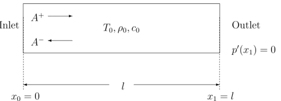
This section presents the basis of the two forcing methods tested in this paper. Consider the inlet of a given domain, located here for convenience at x0 = 0 (Fig. 2). Two techniques

can be utilised to inject velocity perturbations:

• _{The first method (Inlet Velocity Modulation) simply imposes a fluctuating velocity}

at the inlet section. The inlet velocity (in one dimension) has the form :

u(x0, t) = ¯u + u′(x0, t) (1)

where ¯u is the mean velocity and u′_(x

0, t) is the imposed fluctuation (of amplitude

u0) :

u′_(x

(9)

In the linear regime, this boundary condition is representative of a loudspeaker whose membrane moves with the amplitude u0/ω.

• _{The second method (Inlet Wave Modulation) requires the analysis of the unsteady}

flow field at x0 = 0 in terms of acoustic waves. In the limit of linear acoustics, the

unsteady pressure and velocity signals at x0 = 0 are ([2]):

u′_(x

0, t) = _ρ01c0

³

A+_eikx0−iωt₋A−e−ikx0−iωt´ = 1

ρ0c0

³

A+−_A−´_e−iωt ₍₃₎

p′_(x

0, t) = A+eikx0−iωt+ A−e−ikx0−iωt =

³

A++ A−´_e−iωt ₍₄₎

where A+ _{is the amplitude of the wave entering the domain (Fig. 2) and A}− _{is the}

amplitude of the wave leaving the domain ([2]). The basic idea of the IWM method is to impose A+ _{rather than to modulate the velocity fluctuation u}′_(x

0, t). For example,

to impose a modulation at x0 = 0 which would lead to a fluctuating velocity equal to

u0 in the absence of a reflected wave (A− = 0), A+ would be set to ρ0c0u0. In such

cases IVM and IWM give exactly the same result:

A+= ρ0c0u0 and u′(x0, t) = u0e−iωt (5)

In all other cases, however, A− _{is not zero and reflected waves will interact with the}

(10)

to u0eiωt but this will be achieved through the introduction of uncontrolled pressure

waves at the inlet and possible resonances. The next sections show that this can have detrimental effects. For the IWM method, the velocity modulation at the inlet will be (from Eq. (3)): u′_(x 0, t) = u0e−iωt− A− ρ0c0 e−iωt ₍₆₎

It will differ from u0e−iωt because of the velocity contribution due to the reflected

wave A− _{by there will be no coupling between these waves and the inlet forcing:}

in other words, with IWM the ingoing wave train A+ _{will cross the reflected wave}

train A− _{at x}

0 without interaction, an important criterion to avoid resonances. The

IWM method ensures that the incoming wave is pulsated without interacting with the outgoing waves, so that no coupling between the inlet and the rest of the domain is possible. The system might be seen as an infinite tube at the inlet. Outgoing waves (leaving the burner through the inlet) never meet reflecting conditions.

In terms of implementation in a CFD code, IVM is usually straightforward since all codes have the capability of imposing inlet velocities. To use IWM, however, codes must use boundary conditions based on characteristic methods ([2],[22],[25], [1] ) which will not be discussed here.

(11)

3 Isothermal duct

3.1 Analytical solution

Consider a simple duct of constant duct cross section (Fig. 3) in which longitudinal waves travel upstream (amplitude A−_{) and downstream (amplitude A}+_{). Using the assumptions}

of linearised acoustics in the low Mach number approximation, the velocity and pressure fluctuations read : u′_{(x, t) =} 1 ρ0c0 ³ A+eikx−iωt−_A−_e−ikx−iωt´ ₍₇₎ p′_{(x, t) = A}+_eikx−iωt_{+ A}−_e−ikx−iωt ₍₈₎

If the tube ends in a large domain or into the atmosphere, constant pressure (p′ _{= 0) at}

the outlet (x=l) can be assumed. Eq. (7) and (8) can then be solved analytically for an inlet controlled by IVM or IWM:

1. IVM: u′_{(x = 0, t) = u}

0e−iωt. The complex amplitudes A+ and A− are fixed from the

boundary conditions at x = 0 and x = l to obtain:

p′_{(x, t) =} u0ρ0c0

cos(kl)sin(ωt)sin(k(x − l)) (9)

u′_{(x, t) =} u0

(12)

2. IWM: The right going wave amplitude in the duct of Fig. 3 is imposed at the inlet so that A+ ₌ 1

2ρ0c0u0 everywhere. After determining A− with the outlet condition

(p′_{(x = l) = 0), the solution corresponding to this IWM technique is:}

p′_{(x, t) = ρ}

0c0u0sin(kl − ωt) sin(k(x − l)) (11)

u′_{(x, t) = u}

0cos(kl − ωt) cos(k(x − l)) (12)

Note that these conditions can be interpreted in terms of an acoustic wave propagating towards the inlet: For IVM, this wave will meet a fixed velocity (even thought it changes with time), and therefore will be totally reflected. On the other hand, with IWM, this wave will be totally transmitted through the inlet.

3.2 IVM versus IWM solution

Using an IVM or an IWM method to pulsate a combustor in a LES simulation may seem very similar but it is not, especially when pulsing frequencies are close to eigenmodes. In the IVM case, Eq. (9) and (10) show that the amplitudes of the fluctuations depend on the inverse of cos(kl). Since the resonance frequency for the duct of Fig. 3 (with imposed velocity at x = 0 and imposed pressure at x = l) is determined by cos(kl) = 0, amplitudes are very large in the frequency range close to the resonance frequency. Large acoustic

(13)

am-plitudes introduce nonlinear effects between the forcing mode and the eigenmodes which make transfer functions impossible to measure. Furthermore from the numerical point of view it is difficult to introduce a forcing frequency without simultaneously exciting the eigenmodes of a system. Numerical dispersion and effects due to the geometry always transfer energy from the forcing frequency to eigenfrequencies. In any case, if eigenfre-quencies are present, the measured heat release fluctuations (if a flame would have been present) need to be decomposed into contributions due to the forcing frequency and effects due to eigenfrequencies. Such a decomposition is difficult if the flame has a nonlinear response to excitations.

On the other hand, pulsation with a wave, as done in the IWM case (Eq. (11),(12)) fixes only the ingoing wave amplitude A+ _{and permits the wave travelling upstream A}−

to exit the domain of calculation: Eq. (11) and (12) show no amplitude dependence of the solution on the eigenfrequencies of the system. Controlling the amplitudes avoids the excitation of eigenmodes for frequencies close to the eigenfrequencies. From the numerical point of view, an important and useful side effect is the evacuation of artificial non physical high frequencies due to numerical errors at the inlet. One does not need to suppress those errors by artificial viscosity and non dissipative accurate numerical schemes can be used.

(14)

4 Planar flame

The second example is a planar one-dimensional flame (Fig. 4). This configuration has been studied by various authors ([10], [2], [11]). The flame is “compact”: its thickness is supposed to be negligible compared to the acoustic wavelength. The details of the com-bustion process and its interaction with acoustics are modelled via the n − τ formulation. An analytical solution may be obtained in the limit of zero heat release in a constant cross section duct and is extended here for a variable cross section and a non zero heat release in the special case T2 = 4T1.

4.1 Analytical solution

This analytical solution will serve as a basis to demonstrate the difference between IVM and IWM when a flame is present. The configuration is presented in Fig. 4 with a supply tube (left) of length l1, cross section S1, temperature T1, density ρ1 and sound speed c1

connected to a combustion chamber of length l2, cross section S2, temperature T2 = 4T1,

density ρ2 = ρ1/4 and sound speed c2 = 2c1. The classical isentropic equations of linear

(15)

jump conditions [2] require equal pressure on the left and right limit of the intersection:

p′

1(x = l1) = p′2(x = l1) (13)

as well as conserved unsteady volume flow rate with an extra volume source term due to unsteady combustion at the intersection:

S2u′2(x = l1) = S1u′1(x = l1) +

γ − 1 γp0

˙Ω′

T (14)

where p0 is the mean pressure and γ is the isentropic coefficient. The unsteady heat release

˙Ω′

T is usually expressed in terms of the velocity using a n − τ model [10]:

γ − 1 γp0

˙Ω′

T = S1neiωτu′1(l1, t) (15)

where the index of interaction n and the delay τ are input data provided to the model. Solving for the system of Eq. (13),(14),(15), incorporating the reflection coefficients at the inlet (x1 = 0), R1 = A+1/A−1 and the outlet (x2 = l1 + l2), R2 = A+2/A−2e2ik2l2 leads to the

following relation (see appendix A):

Λ = Γ (1 + n e iωτ_{) − 1} Γ (1 + n eiωτ_{) + 1} = e 2ik1l1R1−R2e −2i(k1l1+k2l2) 1 − R1R2e2i(k1l1−k2l2) (16)

which is an equation for the eigenfrequency, where Γ is a dimensionless coefficient depending on cross section, density and sound speed changes.

Γ = S1ρ2c2 S2ρ1c1

(16)

Eq. (16) can be solved by two methods:

1. numerically in the general case: A numerical tool called Soundtube was used to determine frequencies satisfying Eq. (16).

2. in the particular case where the two ducts are of equal length (l2 = l1) and have a

temperature ratio such that T2 = 4T1, an analytical solution can be derived. 1

The second case is used from now on. Let us first determine the eigenmodes of the duct without forcing. The velocity is fixed at the inlet: u′_(x

0 = 0, t) = 0, R1 = 1 and pressure

is fixed at the outlet p′_(x

2 = l1+ l2, t) = 0, R2 = −1. Then the eigenmodes are solutions

of Eq. (16) after simplification:

cos µ1 2k1l1 ¶ · cos2 µ1 2k1l1 ¶ − 3 4− 1 4Λ ¸ = 0 (18)

Eq. (18) shows that the eigenmodes of the duct are composed of two families.

1. One family is due to the left term of the product in Eq. (18). These modes correspond to the half wave mode etc . . . of the first duct and to the quarter wave mode of the second duct: ω1,m = πc1 l1 (2 m + 1) (m = 0, 1, 2, ...) (19) 1

(17)

This mode family always has a velocity node at the flame location. Therefore such modes can not couple to unsteady heat release by the n-τ model. As a result, ω1,m

has no imaginary part (ℑ(ω1,m) = 0). This implies that no amplification or damping

of those modes can occur by flame interaction.

2. The other family is due to the right term in Eq. (18) and corresponds to the fre-quencies: ω2,m = 2c1 l1  ±arccos  ± s 3 4+ 1 4Λ  + 2 m π   (m = 0, 1, 2, ...) (20)

This mode family has real frequencies when there is no unsteady heat release (n = 0 in Eq. 15): ω2,m,0= 2c1 l1  ±arccos  ± s 3 4+ 1 4 Γ − 1 Γ + 1  + 2 m π   (m = 0, 1, 2, ...) (21)

Using perturbation theory one may develop the frequencies (ω2,m = ω2,m,0+ δω2,m)

for small n (small unsteady heat release). This is done in appendix B and results in the following frequency changes:

ℜ_(δω_2,m_{) ≈ −}n c1 2 l1 Γ (Γ + 1)2 cos (ω2,m,0τ ) sin (ω2,m,0l1/2c1) cos (ω2,m,0l1/2c1) (22) ℑ_(δω_2,m_{) ≈ −}n c1 2 l1 Γ (Γ + 1)2 sin (ω2,m,0τ ) sin (ω2,m,0l1/2c1) cos (ω2,m,0l1/2c1) (23)

(18)

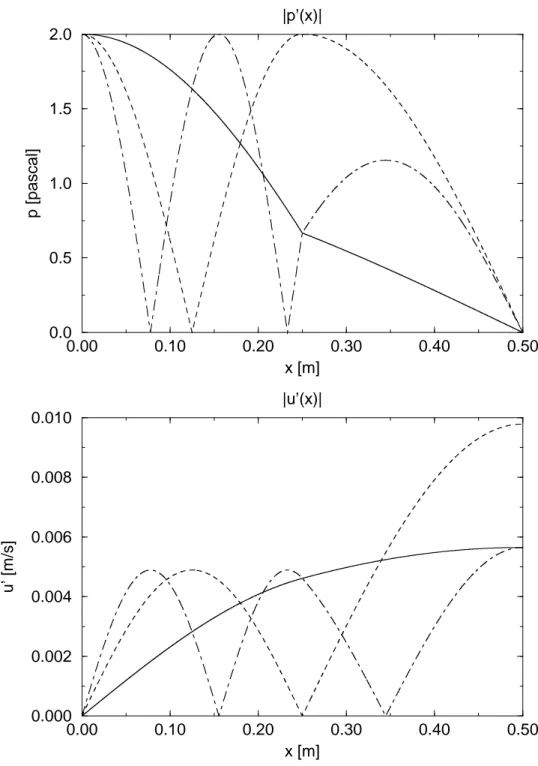
The frequencies of the first six eigenmodes are summarised in table 2. A graphical inter-pretation of the solutions of Eq. 18 is given in figure 5. 2 _{It shows that the frequencies}

of the two mode families overlap. The mode structure of the first three modes is given in figure 6.

4.2 IVM versus IWM solution

The previously derived analytical solution can be used to evaluate the pressure and velocity signal at the duct inlet. Keeping the same boundary condition at the outlet (x = l1+ l2),

that is imposed pressure (p′ _{= 0, R}

2 = −1), the following expressions can be derived for

the pressure fluctuations at the inlet of the first duct (x = 0) and for the two modes of excitation considered in section 2.1:

1. IVM: u′_{(x = 0, t) = u} 1e−iωt p′_{(x = 0, t) = ρ} 1c1u1 i sin³1₂k1l1 ´ h Λ − 3 + 4 sin2³1₂k1l1 ´i cos³1₂k1l1 ´ h 4 cos2³1 2k1l1 ´ −_{3 − Λ}ie −iωt ₍₂₄₎ 2

This analytical solution is very peculiar, because the symmetry induced by the conditions k1l1= 2k2l2,

R1 = 1, R2 = −1 always imposes a velocity node at the flame location for one mode family. This

(19)

2. IWM: A+₁ = ρ1u1c1 p′_{(x = 0, t) = −ρ} 1c1u12i ei( 1 2k1l1−ωt) sin³1 2k1l1 ´ h Λ − 3 + 4 sin2³1 2k1l1 ´i [Λ − e−ik1l1] (25)

The denominator of Eq. (24) goes to zero for eigenfrequencies of the duct (see Eq. (18)). Thus the IVM leads to non finite response in pressure when the forcing frequency is of the order of an eigenfrequency and non-linear effects may pollute the calculation of the duct transfer function. On the other hand the denominator of Eq. (25) is virtually never zero since the modulus of Λ − e−ik1l1 is not zero at resonance frequencies and may never be zero

for n < 1. The modulus of the unsteady pressure p′_(x

0 = 0) at the inlet is plotted for IVM

in Fig. 7 and for IWM in Fig. 8 against the modulation frequency. To verify the quality of the analytical solution (Eq. (24) and (25)) the numerical solver (Soundtube) was also used to solve the linear acoustic equations (7,8) with jump conditions (Eq. (13) and (14)). The result of the numerical solution is added to Fig. 8. An excellent agreement is found between the numerical and analytic solutions. The modulus of the pressure amplitude is finite in the IWM case (Fig. 8). In the IVM case, the amplitude becomes infinite at the frequency associated to the first mode family (cos(k1l1/2), mode 2 in Fig. 7). The modes associated

(20)

because the mode response is plotted for the real frequency axis while the exact singularity is obtained for complex frequencies off the real axis. (e.g. Eq. (23)).

(21)

5 Full CFD application for a laminar burner

The two types of excitation (IVM and IWM) analysed in sections 3 and 4 for two analyt-ically tractable cases (the isothermal duct and the planar flame) are now used in a CFD code in order to study the response of a laminar premixed flame. The numerical tool is briefly discussed in section 5.1, the experimental device used to study the flame is presented in section 5.2 and results are given in section 5.3. 3

5.1 Numerical tool

The numerical tool used in this section is the combustion code AVBP [17] developed at CERFACS. AVBP solves the complete compressible Navier-Stokes equations including chemistry in two and three space dimensions. The capability to handle structured, un-structured and hybrid grids is an important key feature of AVBP. The drawback of higher computational cost compared to structured codes is by far compensated by the capability to calculate complex geometries such as combustors with complex alimentation systems. In the present study, the unstructured approach allows us to compute not only the combustor but also the whole air feeding line as well as the exhaust system (Fig. 10). High order

3

Animated pictures of the numerical simulations can be found on the URL:

(22)

Taylor-Galerkin finite-element schemes allow to keep numerical dissipation and dispersion errors low compared to standard 2nd _{order centred difference schemes [18]. It is important}

to use such schemes in order to minimise errors in the simulations of transfer functions.

5.2 The experimental burner

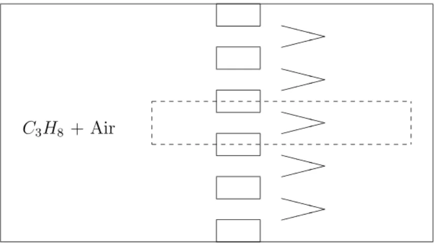
The burner considered for the comparison between IVM and IWM is described by Le Hel-ley in his thesis [3]. The burner BH3P consists of a ducted premixed propane-air flame and operates at different fuel mixture fractions. Flame stabilisation is produced by a per-forated plate with multiple holes (Fig. 9). For certain operation modes this burner features small laminar Bunsen tip flames behind each hole and no turbulence effects are present. We limit our study to this regime. A cut sketch of the half burner is given in Fig. 10. In the experiment, the flame is excited by a loudspeaker located upstream (Point A in Fig. 10). The axisymmetrical computational mesh has been chosen such that chemistry and thermodynamic effects are resolved on the mesh (10515 nodes). To simplify this task, chemistry is modelled using a single-step Arrhenius law ( ˙ω = AYα

FY β

O exp(−T /Ta)) where

the preexponential constant is A = 9.67 1010_{uSI, the mass fraction exponents are α = 0.5,}

(23)

produce the right flame speed in the range of equivalence ratios of Le Helley’s experiment. Pulsation amplitudes imposed at the inlet section are kept to 10% of mean air flow (4m/s) and thus lay well within the linear acoustic domain.

5.3 Comparison of IVM and IWM

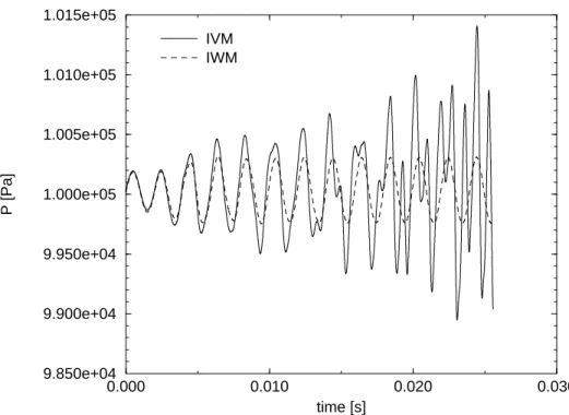
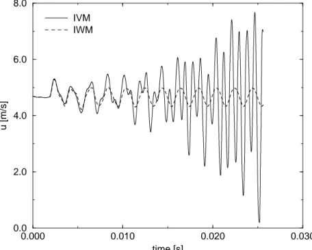
The boundary conditions for the mean flow correspond to standard conditions for CFD: imposed inlet velocities and outlet pressure. At the outlet pressure is imposed as proposed in the NSCBC method ([2],[24],[22]). The inlet is treated with characteristic boundary conditions [22] in order to superimpose either velocity modulation (in the IVM case) or acoustic fluctuations (in the IWM case) to the mean flow. Fig. 11 shows the pressure signal at the inlet (Point A in Fig. 10) obtained with IVM and IWM at the frequency of 500 Hz for an amplitude u0 = 0.4m/s. Fig. 12 shows the velocity signal at the inlet (Point A)

obtained with IVM and IWM at the frequency of 500 Hz.

During the first instants of the simulation (≈ 2ms) the inlet pressure and velocity signals are almost identical for IVM and IWM (Fig. 11) because no wave is reflected from the chamber to the inlet (A− _{= 0 in Fig. 2). When the first reflected waves have reached the}

(24)

inlet after travelling upstream (around t = 5ms ) the differences between IVM and IWM show up. In the IVM case, as expected, the velocity signal at the inlet follows the imposed sinusoidal modulation (solid line in Fig. 12). However the pressure at the inlet increases in amplitude (solid line in Fig. 11) and other frequencies appear.

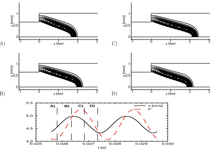
In Fig. 15 snapshots at different instants in the forcing cycle are given for IWM. The isolines show the instantaneous reaction rates and therefore the position of the flame be-hind the flame holder. In the graph below the velocity signal a the flame holder and the integrated heat release are given in time. The vertical lines in the graph correspond to the instantaneous snapshots. One sees the time delay of the heat release to the the velocity signal at the flame holder.

Concerning the measurement of the transfer function the velocity signal (Fig. 14) and pressure signal (Fig. 13) at the flame holder (Point B in Fig. 10) are far more important since they are the reference values to be used together with the integral heat release to determine the transfer function parameters n and τ of the burner. In the IVM case the amplitude of the velocity increases at the flame holder and other frequencies are super-imposed on the forcing frequency (solid line in Fig. 14). At the flame holder, the actual amplitude of the flow oscillation is not u0 = 0.4m/s as imposed at the inlet but, because

(25)

of acoustic reflections in the system, reaches values of the order of 4m/s. A closer ex-amination by Fougere methods [26] of the velocity signal at the flame holder ( Fig. 14) shows the appearance of a 1117 Hz mode for the IVM case. This is consistent with the numerical acoustic analysis of the domain with Soundtube presented in table 3. Using the boundary conditions R1 = 1 (u′(xin) = 0) and R2 = −1 (p′(xout) = 0), the first unstable

mode with positive imaginary part is obtained at f = 1118.6Hz (mode 5). This confirms that the IVM technique excites the combustor at 500Hz (as expected) but also forces the first unstable eigenmode (mode 5) of the combustor at 1118Hz. The reason why the 6th

mode does not appear in the spectral analysis of the velocity signal at point B is not clear. Note however that the 5th_{mode is close to the second harmonic of the excitation frequency}

which may feed the 5th _{mode more efficiently than the 6}th _{mode. This IVM simulation is}

obviously not suited to flame transfer measurements. On the other hand, in the IWM case, the pressure and velocity signals in Fig.(13) and (14) (dotted line) at the flame holder are virtually monochromatic (f = 500Hz) and keep a constant amplitude. As expected from the examples of Sections 3 and 4, no eigenmodes are excited when the IWM technique is used. Thus the response of the flame can be accessed easily through a classical FFT-based spectral analysis in terms of n and τ . This confirms the superiority of the IWM to IVM.

(26)

5.4 Transfer function measurement

The case of fuel excess (φ = 1.2) of Le Helley is now chosen to evaluate the flame transfer function. In this regime the burner admits small Bunsen tip flames over every hole. The calculation is limited to an axisymmetric domain of one single burner hole keeping the burner length for acoustic reasons. To simulate a symmetry between the holes, slip walls are imposed at all sections except at the flame holder which consists of non slip walls with imposed heat resistance. This configuration is acoustically equivalent to the experimental burner of Le Helley but neglects all interactions between individual Bunsen tip flames. In the experiment of Le Helley, a hot wire anemometer was placed 1.5 cm before the flame holder to measure the velocity (u′_{(t)). Integral heat release fluctuations were measured by}

a photo multiplier tube. In the calculation temporal signals of integral heat release and velocity are stored. Calculations at the forcing frequencies of f = 100, 250 and 500 Hz are performed using the IWM method. Comparison of integral heat release fluctuations (R

˙ω′_{dV ) to velocity fluctuations (u}′_{(t)) then give the transfer function parameters n and}

τ defined by : neiωτ = γ − 1 S1γp0 R ˙ω(t)dV u′_(t) (26)

(27)

where ˙ω is the local unsteady heat release. Values for the transfer function parameter are given in Fig. 16. The values for the transfer function obtained by experiment and calcu-lation are comparable. The delay τ predicted numerically seems constant with frequency while it is non constant in experiment. This may be due to a constant phase of small value between velocity signal and integral heat release in the experiment. The values of n obtained from the calculation are of the same order of magnitude as the experiment. The tendency of decreasing n at high frequencies is reproduced by the calculation. 4 _{It is not}

possible to use the IVM method for measuring the transfer function parameters since no

4

Replacing integral heat release by fuel consumption in Eq. 26 and balancing fuel consumption with

fuel supply leads to :

QS1u1ρ0YF =

Z

˙ωdV (27)

Then in the low frequency limit (ω → 0), an estimate can be derived for the limit value of the interaction

index n : n(ω → 0) = γ − 1 γp0 Q ∗ ρ 0Y 0 Fmin (1, 1/φ) (28)

Assuming constant heat capacity ¡Cp(T2_{− T}1) = QY 0

F min (1, 1/φ)¢ the previous equation (28) can be

written:

n(ω → 0) = T2 T1

− 1 (29)

In this case the low frequency limit is n0= 5.99 (Fig 16). This value is of the same order as experimental

(28)

harmonic regime at the forcing frequency is obtained (solid line in Fig. 14).

6 Conclusion

Two techniques to introduce pulsation in a combustion chamber computation were tested: the first one (IVM) directly modulates the inlet velocity, while the second one (IWM) mod-ulates the acoustic wave entering the chamber. Two analytical and one numerical cases were used to test IVM and IWM. Results show that IVM leads to resonance phenomena perturbing measurements of transfer functions. Pulsation with a wave (IWM) is an al-ternative technique that assures finite amplitudes and monochromatic signals for transfer function determination. Analytical expressions and numerical calculations of AVBP are compared to a 1D acoustic code with good agreement. The application of IWM to the laminar burner of Le Helley showed that transfer functions can be predicted accurately using IWM, while IVM leads to the excitation of eigenmodes of the burner which prevent prediction of transfer functions. More generally, theses results suggest that extreme care must be taken in CFD codes to compute unsteady reacting flows since boundary condi-tions largely control the solution. Implementing boundary condicondi-tions able to control waves crossing the boundaries appears to be a necessary step in such numerical tools [2], [1].

(29)

References

[1] F. Nicoud. Defining wave amplitude in characteristic boundary conditions. Journal of Computational Physics, 149(2):418–422, 1999.

[2] T. Poinsot and D. Veynante. Theoretical and Numerical Combustion. Edwards, 2001 edition, 2001.

[3] Ph. Le Helley. Etude théorique et expérimentale des instabilités de combustion et de leur contrôle dans un brûleur laminaire prémélangé. PhD thesis, Laboratoire d’Energétique Moléculaire et Macroscopique, Combustion (E.M2.C), UPR 288, CNRS et Ecole Centrale Paris, 1994.

[4] G.J. Bloxsidge, A.P. Dowling, and P.J. Langhorne. Reheat buzz: an acoustically coupled combustion instability. part 2: Theory. Journal of Fluid Mechanics, 193:445– 473, 1988.

[5] H.J. Merk. An analysis of unstable combustion of premixed gases. Sixth Symposium on Combustion 1956, 6:500–512, 1956.

[6] Y. Matsui. An experimental study on pyro-acoustic amplification of premixed laminar flames. Combustion and Flame, 41, 1981.

[7] A.P. Dowling. Nonlinear self-excited oscillations of a ducted flame. Journal of Fluid Mechanics, 346:271–290, 1997.

[8] S. Ducruix, D. Durox, and S. Candel. Theoretical and experimental determinations of the transfer function of a laminar premixed flame. Proceedings of the Combustion Institute, 28:765–773, 2001.

[9] Sir James Lighthill. Waves in fluids. Cambridge University Press 1978, 1979 edition, 1978.

[10] K. R. McManus, T. Poinsot, and S. M. Candel. A review of active control of combus-tion instabilities. Prog. Energy Combust. Science, 19:1–29, 1993.

[11] A.P. Dowling. The calculation of thermoacoustic oscillations. Journal of Sound and Vibration, 180(4):557–581, 1995.

[12] M. Fleifil, A.M. Annaswamy, Z.A. Ghoneim, and A.F. Ghoniem. Response of a laminar premixed flame to flow oscillations: A kinematic model and thermoacoustic instability results. Combustion and Flame, 106:487–510, 1996.

[13] V.K. Chakravarthy and S. Menon. Subgrid modeling of turbulent premixed flames in the flamelet regime. Flow, Turbulence and Combustion, 65(2):133–161, 2000.

[14] H. Forkel and J. Janicka. Large-eddy simulation of a turbulent hydrogen diffusion flame. Flow, Turbulence and Combustion, 65(2):163–175, 2000.

(30)

[15] K. Mahesh, G. Constantinescu, and P. Moin. Large-eddy simulation of gas turbine combustors. CTR, Annual Research Briefs, pages 219–228, 2000.

[16] C.D. Pierce and P. Moin. Large eddy simulation of a confined coaxial jet with swirl and heat release. AIAA Fluid Dynamics Conference, Albuquerque NM, AIAA 98-2892, 1998.

[17] T. Sch¨onfeld and M. Rudgyard. Steady and unsteady flows simulations using the hybrid flow solver AVBP. AIAA Journal, 37(11):1378–1385, 1999.

[18] O. Colin and M.Rydgyard. Development of high-order taylor-galerkin schemes for LES. Journal of Computational Physics, 162:338–371, 2000.

[19] F. Nicoud and F. Ducros. Subgrid-scale stress modelling based on the square of the velocity gradient tensor. Flow, Turbulence and Combustion, 62:183–200, 1999.

[20] O. Colin, F. Ducros, D. Veynante, and T. Poinsot. A thickened flame model for LES of turbulent premixed combustion. Physics of Fluids, 12(7):1843–1863, 2000.

[21] J.P. Legier, T. Poinsot, and D. Veynante. Dynamically thickened flame LES model for premixed and non-premixed turbulent combustion. Center of Turbulence Research, Proceedings of the summer program 2000, pages 157–168, 2000.

[22] T. Poinsot and S. Lele. Boundary conditions for direct simulations of compressible viscous flows. Journal of Computational Physics, pages 104–129, 1992.

[23] T. Sch¨onfeld and T. Poinsot. Influence of boundary conditions in LES of premixed combustion instabilities. Center of Turbulence Research, Annual Research Briefs 1999, pages 73–84, 1999.

[24] F. Nicoud and T. Poinsot. Boundary conditions for compressible unsteady flows. In L. Halpern, F. Nataf and L. Tourrette Editors, Novascience, Artificial Boundary Conditions at Interfaces, 2001. in press.

[25] K.W. Thompson. Time dependent boundary conditions for hyperbolic systems. J. Comput. Phys., 68:1–24, 1987.

[26] D. Veynante and S. M. Candel. Application of nonlinear spectral analysis and signal reconstruction to laser doppler velocimetry. Experiments in Fluids, 6:534–540, 1988. [27] D. Veynante and T. Poinsot. Large eddy simulation of combustion instabilities in

turbulent premixed burners. Center of Turbulence Research, Annula Research Briefs 1997, pages 253–274, 1997.

[28] M.K.Myers. On the acoustic boundary condition in the presence of flow. Journal of Sound and Vibration, 71(3):429–434, 1980.

(31)

A

Derivation of the implicit two tube frequency

rela-tion for the planar flame

Taking the jump conditions (Eq. (13),(14)) and rewriting them with the linear acoustic notation and the n − τ model (15) one has:

A+₁eik1l1 + A− 1e−ik 1l1 = A+₂ + A− 2 (30) S2 ρ2c2 ³ A+₂ −_A− 2 ´ = S1 ρ1c1 ³ A+₁eik1l1 ₋ A− 1e−ik 1l1´ + S1neiωτu1(x = l1) (31) = S1 ρ1c1 ³ A+ 1eik 1l1 ₋ A− 1e−ik 1l1´ + ne iωτ_S 1 ρ1c1 ³ A+ 1eik 1l1 ₋ A− 1e−ik 1l1´ = S1(1 + ne iωτ₎ ρ1c1 ³ A+₁eik1l1 ₋ A− 1e−ik 1l1´

One may rewrite this system in a matrix like system as noted in [10], [2] using the definition (17): Ã A+2 A− 2 ! = 1 2 Ã

eik1l1(1 + Γ (1 + neiωτ)) e−ik1l1(1 − Γ (1 + neiωτ))

eik1l1 (1 − Γ (1 + neiωτ_{)) e}−ik1l1 (1 + Γ (1 + neiωτ₎₎ ! Ã A+1 A− 1 ! (32) Using the definitions of the reflection coefficients R1 = A+1/A−1, R2 = A+2/A−2e2ik2l2 and

regrouping of the terms containing (1 − Γ(1 + n eiωτ_{)), (1 + Γ(1 + n e}iωτ_{)) one may reduce}

Eq. (32) to ³ 1 + Γ³1 + neiωτ´´µ eik1l1 ₋ R2 R1 e−2ik2l2+ik1l1 ¶ = (33) ³ 1 − Γ³1 + neiωτ´´ µ R2e−2ik2l2+ik1l1 − 1 R1 e−ik1l1 ¶

which leads to Eq. (16). The analytical solutions presented in section 4.1, Eq. (16) can be generalised to the case when k1l1 = 2 k2l2. Then Eq. (16) may be written as:

Γ (1 + n eiωτ_{) − 1} Γ (1 + n eiωτ_{) + 1} = e 2ik1l1R1−R2e −3ik1l1 1 − R1R2eik1l1 (34) = R1e 3 2ik1l1 −R 2e− 3 2ik1l1 1e−12ik1l1 −R 1R2e 1 2ik1l1

Choosing any combination of R1, R2 = ±1 leads to an explicit form for the resonance

frequency when there is no unsteady heat release using the addition theorems for trigono-metric functions. Those are given in table (4).

(32)

B

Derivation of the growth amplitude

The growth amplitude may be developed for all cases given in table (4). In the linear case the growth amplitude is the imaginary part of the frequency (modulo 2π). If the imaginary part is positive this leads to a positive growth amplitude and the mode is unstable. If the imaginary part is negative the mode is stable.

Here we develop the growth rate for the case given in section (4.1). Linear development around an eigenfrequency ω2,m,0 given by Eq. 20 , ω2,m = ω2,m,0+ δω2,m leads to :

cos ((ω2,m,0+ δω2,m)l1/2c1)  cos2((ω_2,m,0+ δω_2,m)l₁/2c₁) − 3 4− 1 4 Γ³1 + n ei(ω2,m,0+δω2,m)τ´₋₁ Γ (1 + n ei(ω2,m,0+δω2,m)τ) + 1  = 0 (35) Linear development of the cos2_((ω

2,m,0+ δω2,m)l1/2c1) term neglecting high order terms

leads to : cos2((ω2,m,0+ δω2,m)l1/2c1) ≈ cos2(ω2,m,0l1/2c1)− δω2,ml1 c1 cos (ω2,m,0l1/2c1) sin (ω2,m,0l1/2c1) (36) Now one has to distinguish between the two families of modes . For the first family one has cos (ω1,0l1/2c1) = 0 and the growth amplitude is always zero. For the second mode

family one has:

cos (ω2,m,0l1/2c1) = ± s 3 4 + 1 4 Γ − 1 Γ + 1 (37)

We assume that n is small compared to the geometric restraints (n ≪ 1−1/Γ) and linearise Λ. Γ (1 + n eiω2,mτ) − 1 Γ (1 + n eiω2,mτ) + 1 ≈ Γ − 1 Γ + 1 + 2Γ n eiω2,m,0τ (Γ + 1)2 (38)

Splitting δω2,m= δω2,m,r + iδω2,m,i one derives the growth rate of Eq. (36) :

ℑ_(δω_2,m_{) ≈ −} c1 2 l1 1 sin (ω2,m,0l1/2c1) 1 cos (ω2,m,0l1/2c1) Γ n sin (ω2,m,0τ ) (Γ + 1)2 (39)

as well as the real frequency shift: ℜ_(δω_2,m_{) ≈ −} c1 2 l1 1 cos (ω2,m,0l1/2c1) 1 sin (ω2,m,0l1/2c1) Γ n cos (ω2,m,0τ ) (Γ + 1)2 (40)

(33)

1 Isothermal duct (section 3): Analytical solution T0, ρ0, c0

1 2 Planar premixed flame (section 4): Analytical solution

T2 = 4T1, ρ1 = 4ρ2, c2 = 2c1

✟✟✟

❍❍❍ V flame (section 5): CFD calculation

laminar, premixed

Table 1: Investigated cases for IVM versus IWM

mode nbr family frequency

1 2 ω = 2c1 l1 arccos ³q 3 4 + 1 4Γ−1Γ+1 ´ 2 1 ω = 2c1 l1 π 2 3 2 ω = 2c1 l1 arccos ³ −q3 4 + 1 4Γ−1Γ+1 ´ 4 2 ω = 2c1 l1 h 2π − arccos³−q3 4 + 1 4Γ−1Γ+1 ´i 5 1 ω = 2c1 l1 3π 2 6 2 ω = 2c1 l1 h 2π − arccos³q3 4 + 1 4Γ−1Γ+1 ´i

Table 2: Eigenmodes of the plane flame example without unsteady heat release.

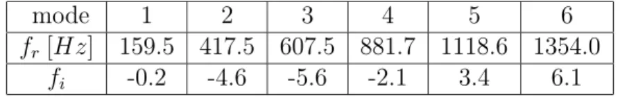
mode 1 2 3 4 5 6

fr[Hz] 159.5 417.5 607.5 881.7 1118.6 1354.0

fi -0.2 -4.6 -5.6 -2.1 3.4 6.1

Table 3: Real and imaginary parts of the eigenfrequencies of the experimental setup deter-mined by the 1D acoustic code (Soundtube) with the reflection coefficients R1 = 1 (u′(x =

0) = 0) and R2 = −1 (p′(x = l) = 0). The values of n = 4.0 and τ = 0.5ms were taken

(34)

R1 R2 ω1 ω2 1 1 2nπc1 l1 2c1 l1 arcsin ± q 3 4 − 1 4Λ -1 1 (2n+1)πc1 l1 2c1 l1 arccos ± q 3 4 − 1 4Λ 1 -1 (2n+1)πc1 l1 2c1 l1 arccos ± q 3 4 + 1 4Λ -1 -1 2nπc1 l1 2c1 l1 arcsin ± q 3 4 + 1 4Λ

Table 4: Explicit dispersion relations for the case l2/c2 = l1/2c1

a) real burner:

Plenum inlet duct

combustion chamber Section 1 ✁ ✁ ✁ ✁☛ ✟✟✟ ❍❍❍

b) simulated combustion chamber

artificial computational inlet

✟✟✟ ❍❍❍

(35)

+

A

−

Outlet Inlet Combustion Chamber Flame Front Burnt Gases Cold Gases l x = 0 x = l x = l + l 0 1 1 1 2 1 2 2 l

Figure 2: typical burner configuration: The flame is usually anchored aerodynamically (swirled inlet) or thanks to a bluff body.

Inlet _T₀_{, ρ}₀_{, c}₀ A− ✛ A+ ✲ Outlet p′_(x 1) = 0 ✛ l ✲ x0 = 0 x1 = l

(36)

Inlet _T₁_{, ρ}₁_{, c}₁ A− 1 ✛ A+1 ✲ T2, ρ2, c2 A− 2 ✛ A+2 ✲ Outlet p′_(x 2) = 0 ✛ l1 ✲✛ l2 ✲ x0 = 0 x1 = l1 x2 = l1+ l2

Figure 4: Configuration for the analytical solution with a planar flame.

0.0 1.0 2.0 3.0 4.0 5.0 6.0 −1.0 −0.5 0.0 0.5 1.0 q 3 4 + 1 4 Γ−1 Γ+1 −q3 4 + 1 4Γ−1Γ+1

Figure 5: Mode distribution: The modes are given in table 2. The first family of modes is given when cos(1/2k1l1) = 0, here represented by squares. These nodes have zero

amplification. The second family of modes is given for cos(1/2k1l1) = ±

q 3 4 + 1 4 Γ−1 Γ+1, here

(37)

0.00 0.10 0.20 0.30 0.40 0.50 x [m] 0.000 0.002 0.004 0.006 0.008 0.010 u’ [m/s] |u’(x)| 0.00 0.10 0.20 0.30 0.40 0.50 x [m] 0.0 0.5 1.0 1.5 2.0 p [pascal] |p’(x)|

Figure 6: Structure of the first three modes. The first mode (family 2) is plotted with a solid line, the second mode (family 1) is plotted by a dashed line, and the third mode (family 2) is plotted by a dot-dashed line. The top figure shows the absolute value of the pressure amplitude, while the bottom figure shows the absolute value of the velocity amplitude. The amplitudes are given by fixing the upstream pressure wave amplitude A+ _{= 1.}

(38)

0.0 500.0 1000.0 1500.0 2000.0 f [Hz] 0.0 5.0 10.0 15.0 20.0

non dimensional pressure amplitude ||p’

|| numeric tool analytic formula mode 1: 270 Hz mode 2:694 Hz mode 3: 1132 Hz mode 4: 1669 Hz

Figure 7: inlet pressure amplitude with the IVM method, symbols: analytic solution of Eq. (24), solid line: numerical solution obtained with Soundtube, (n = 0.5, τ = 0.001s, l1 =

0.25m, T1 = 300K, ρ1 = 1.177kg/m3). 0.0 500.0 1000.0 1500.0 2000.0 f [Hz] 0.0 1.0 2.0 3.0

non dimensional pressure amplitude ||p’

||

numeric tool analytic formula

Figure 8: inlet pressure amplitude with the IWM method, symbols: analytic solution of Eq. (25), solid line: numerical solution obtained with Soundtube, (n = 0.5, τ = 0.001s, l1 =

(39)

C3H8 + Air ✘✘✘ ✘✘✘ ✘✘✘ ✘✘✘ ✘✘✘ ❳❳❳ ❳❳❳ ❳❳❳ ❳❳❳ ❳❳❳

Figure 9: Sketch of the flameholder. The computational domain is given by the dashed box. ✁ ✁ ✂✄✂ ✂✄✂ ✂✄✂ ✂✄✂ ✂✄✂ ✂✄✂ ✂✄✂ ✂✄✂ ✂✄✂ ✂✄✂ ✂✄✂ ✂✄✂ ☎✄☎ ☎✄☎ ☎✄☎ ☎✄☎ ☎✄☎ ☎✄☎ ☎✄☎ ☎✄☎ ☎✄☎ ☎✄☎ ☎✄☎ ☎✄☎ Flame Exitation Flameholder Inlet Outlet l=0.65 m air + propane symmetry axis Point A Point B walls r = 1mm Point C

Figure 10: A sample burner for a laminar propane air flame with a constant pressure outlet (p′ _{= 0). The inlet is excited by wave or velocity pulsation leading to different flame}

(40)

0.000 0.010 0.020 0.030 time [s] 9.850e+04 9.900e+04 9.950e+04 1.000e+05 1.005e+05 1.010e+05 1.015e+05 P [Pa] IVM IWM

Figure 11: Pressure at the duct inlet (Point A) for IVM and IWM for a forcing frequency of 500 Hz and a forcing amplitude of 0.4m/s.

0.000 0.010 0.020 0.030 time [s] 3.5 4.0 4.5 5.0 u [m/s] IVM IWM

Figure 12: Velocity signal at the duct inlet (Point A) for IVM and IWM for a forcing frequency of 500 Hz and a forcing amplitude of 0.4m/s

(41)

0.000 0.010 0.020 0.030 time [s] 9.960e+04 9.980e+04 1.000e+05 1.002e+05 1.004e+05 P [Pa] IVM IWM

Figure 13: Pressure at the flame holder (Point B) for IVM and IWM for a forcing frequency of 500 Hz and a forcing amplitude of 0.4m/s.

0.000 0.010 0.020 0.030 time [s] 0.0 2.0 4.0 6.0 8.0 u [m/s] IVM IWM

Figure 14: Velocity signal at the flame holder (Point B) for IVM and IWM for a forcing frequency of 500 Hz and a forcing amplitude of 0.4m/s.

(42)

A) x [mm] y [m m ] -1 0 1 2 3 0 0.5 1 C) x [mm] y [m m ] -1 0 1 2 3 0 0.5 1 B) x [mm] y [m m ] -1 0 1 2 3 0 0.5 1 D) x [mm] y [m m ] -1 0 1 2 3 0 0.5 1 0.025 0.026 0.027 0.028 0.029 0.030 t [s] 4.0 4.5 5.0 5.5 u [m/s] F’ A) B) C) D)

Figure 15: above: snapshots of with isolines of reaction rates at different times in a cycle of a flame pulsed with a wave. underneath: velocity signal at the flame holder and the reduced heat release F′ _{= Ω (S}

(43)