Carbon and electron flow via methanogenesis, So₄²⁻, NO₃⁻ and Fe³⁺ reduction in the anoxic hypolimnia of upper Mystic Lake

CARBON AND ELECTRON FLOW VIA METHANOGENESIS,

S042,

N0

~, AND Fe

-REDUCTION IN THE ANOXIC

HYPOLIMNIA OF UPPER MYSTIC LAKE

by

Eliza J.R. Peterson B.S. Microbiology University of Michigan, 2002

SUBMITTED TO THE DEPARMENT OF CIVIL AND ENVIRONMENTAL ENGINEERING IN PARTIAL FULFILLMENT OF THE REQUIREMENTS FOR THE

DEGREE OF

MASTER OF SCIENCE IN CIVIL AND ENVIRONMENTAL ENGINEERING AT THE

MASSACHUSETTS INSTITUTE OF TECHNOLOGY

JUNE 2005

MASSACHUSETTS I OF TECHNOL © 2005 Massachusetts Institute of Technology

All rights reserved

MAY

3

1 2(

19

Department of Civil and Environmental Engineering May 12, 2005

'I,,

Harold Hemond

LIBRARIES

CARBON AND ELECTRON FLOW VIA METHANOGENESIS,

S0 42

, N0

, AND Fe

REDUCTION IN THE ANOXIC

HYPOLIMNIA OF UPPER MYSTIC LAKE

By

Eliza J.R. Peterson

Submitted to the Department of Civil and Environmental Engineering on May 12, 2005 in Partial Fulfillment of the Requirements for the Degree of Master of Science in Civil

and Environmental Engineering

ABSTRACT

The profiles of CH4 and CO2 obtained by the use of a novel sampler, along with the profiles for nitrate (N03-), sulfate (SO43) and iron (Fe 2 _{) were used to estimate the}

rates of the various anaerobic decomposition reactions during spring and fall stratification in Upper Mystic Lake. The equivalent electron and carbon flow of the reactions were also calculated to obtain a mass balance within the hypolimnia of UML. From the calculations, the approximate organic carbon decomposition rate, measured as CO2 accumulation, was 7.54 mmol m-2 d-I. The amount of decomposition from the reactions involving nitrate, sulfate, iron and methane formation together accounted for 80% of the total organic carbon decomposition. Therefore, 20% of the CO2 accumulation in UML could not be accounted for. Possible explanations for the excess CO2 production could be the formation of reduced iron minerals and/or the loss of methane due to ebullition and oxidation. Such explanations suggest future studies of UML to better resolve the electron budget.

In order to study the redox balance in Upper Mystic Lake, a method was devised for precisely sampling dissolved gases in the water column. Like other stratified lakes, UML has a large amount of anaerobic metabolism of organic matter occurring in the sediments and a subsequent accumulation of methane (CH4) and carbon dioxide (C0 2) in

the hypolimnia. Previously, limnological sampling for dissolved gases involved filling glass bottles with water pumped from depth using a peristaltic pump; however, such methods introduce the potential for gas exchange with the atmosphere. Therefore, there was a need for a dissolved gas sampler that could be used to obtain samples at precise depth intervals while at the same time isolating the samples from outside influences.

Thesis Supervisor: Harold Hemond

ACKNOWLEDGEMENTS

My sincerest and deepest thanks go to my advisor, Professor Harry Hemond, with whom it was a pleasure and privilege to work. His combination of intellect, kindness,

and humor is incredible. I am very appreciative of the opportunity afforded me to work with him and on Upper Mystic Lake.

I am also indebted to Larry Linden and the Martin Family for Linden and Martin

Fellowships.

I have enjoyed my time and knowing many people at the Parsons Lab; several deserve special gratitude for their help and friendship: Katherine Lin, Janet Chuang, Matt Orosz, and Terry Donoghue. I would also like to acknowledge a UROP assistant,

Elizabeth Walker for her help with sulfate analysis. In addition, Dr. John Durant, Michele Cutrofello, and Theresa McGovern of Tufts University deserve recognition for their collaboration with the Tufts Nutrient Project.

Above all, this thesis would not have been completed without a vast amount of love and support from my family, especially from my parents, Jane and Paul Peterson; my sister, brother-in-law and niece, Amy, Jeff and Ana Dunfee, and my sister, Carrie Peterson.

TABLE OF CONTENTS

A b stra ct...2

A cknow ledgem ents... 3

T able of C ontents...4

L ist o f Figures...6

L ist o f T ables... . .7

I. Introduction .. :... .9

II. Stu d y Site ... . . 12

III. M ethod s... . . 14

Limnological Sampling... 14

Nitrate, Sulfate and Ammonium...14

Iron (II)... . . 15

Methane and Carbon Dioxide...15

IV . C alculatio ns... .23

V . R esults... . . 26

T, 02, pH and Conductivity Profiles...26

Inorganic Nitrogen Profiles...30

Fe 2 P rofiles...33

S 42- P rofile s...3 5 CH4 and CO2 Profiles...38

Rates of Decomposition and Reduction of Electron Acceptors...41

C arbon Flow ... ... ... 49

V I. D iscussion ... .5 1 Comparison to Other Lakes...51

Possible Explanations for the Electron Imbalance... ... 54

V II. C onclusion ... 57

V III. A ppendix A ... ... ... 5 8 The Dissolved Gas Sampler...58

IX . A ppendix B ... 67

Summary of Limnological Data... ... ... ... 67

LIST OF FIGURES

Figure 1: Upper Mystic Lake bathymetry...13

Figure 2: Acidified vs. non-acidified CO2 samples...18

Figure 3: Chromatogram of lower column...19

Figure 4: Chromatogram of upper column...20

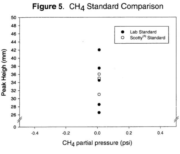
Figure 5: CH4 standard comparison...21

Figure 6: CO2 standard comparison...22

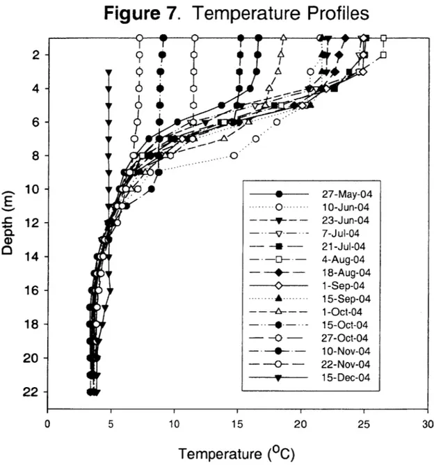
Figure 7: Temperature Profiles...27

Figure 8: Temperature Contour...28

Figure 9: Dissolved Oxygen Profiles...29

F igure 10: N H 4' Profiles...31 F igure 11: N O 3~Profiles...32 Figure 12: Fe2 + Profiles...34 F igure 13: SO 42- Profiles...36 Figure 14: C -4 Profiles...39 Figure 15: C O 2 Profiles...40

Figure 16: Change in hypolimnetic mass of C0 2, CH 4 during 110 day sam pling period...42

Figure 17: Change in hypolimnetic mass of 02, NO3, SO4 -, Fe2+ during 110 day sampling period...43

Figure A-1: The Dissolved Gas Sampler Diagram...63

Figure A-2: The Dissolved Gas Sampler...64

Figure A-3: Syringe "dock"...65

LIST OF TABLES Table 1: Oxidation-reduction reactions involving the

decomposition of organic matter...11

Table 2: UML bathymetry data used for mass balance calculations...25

Table 3: Late September 2004 storm data...37

Table 4: Rates of change of hypolimnetic species...44

Table 5: Comparison of CO2 accumulation in other lakes...45

Table 6: Reducing equivalents necessary to reduce the molar quantities of electron acceptors...48

Table 7: Carbon equivalents produced during the reduction of electron acceptors... 50

Table 8: Comparison of overall electron budget from several lakes...52

Table 9: Comparison of electron acceptors as percent of CO2 accumulation for the Canadian experimental lakes...53

Table A-1: Cost and parts list for sampler...66

Table B-1: 13-May-04 Profile...68

Table B-2: 27-May-04 Profile...69

Table B -3: 10-Jun-04 Profile...70

Table B-4: 23-Jun-04 Profile...71

Table B-5: 7-Jul-04 Profile...72

Table B-13: Table B-14: Table B-15: Table B-16: Table B-17: Table B-18: Table B-19: Table B-20: Table B-21: Table B-22: Table B-23: Table B-24: Table B-25: Table B-26: 15-Sep-04 P rofile...80

15-Sep-04 Profile continued... .... 81

1-O ct-04 Profile... 82

1-Oct-04 Profile continued...83

15-O ct-04 Profile... 84

15-Oct-04 Profile continued...85

27-O ct-04 Profile... 86

27-Oct-04 Profile continued...87

10-N ov-04 P rofile...88

10-Nov-04 Profile continued...89

22-Nov-04 Profile...90

22-Nov-04 Profile continued...91

15-Dec-04 Profile...92

I. INTRODUCTION

The cycling of energy, carbon and nutrients in lake ecosystems is dependent on the decomposition of organic matter. In lake hypolimnia, decomposition is a dominant process and strongly influences the chemical constituents therein. The decomposition of organic matter involves microbial reactions that consume electron acceptors (e.g. 02,

3- 3+

N0 3, SO4 , Fe

)

thermally stratified, the transport of metabolic end products from the hypolimnion to the upper portion (the epilimnion), and the downward diffusion of oxygen and other electron acceptors into the hypolimnion is small (Mattson and Likens, 1993; Houser J et al., 2003). Thus, hypolimnetic concentrations of oxygen and other electron acceptors typically decrease over the course of the stratified season while C0 2, CH4., and the reduced end products accumulate.

methanogenesis, nitrate, sulfate and iron reduction during anaerobic decomposition of organic matter in the hypolimnion of Upper Mystic Lake (UML; Medford,

Massachusetts, USA) during the stratified period. This is done by constructing a mass balance model from changes in the vertical profiles of nitrate, sulfate, ferrous iron (Fe2_,) and methane during the entire sampling period.

Table 1. Oxidation-reduction reactions involving the

decomposition of organic matter.

Table 1 includes the CO2 equivalents and the maximum amount of free energy (AGo) that can be derived from the reactions.

Reaction: Aerobic oxidation of organic matter

(CH2O)106(NH3)16(H3PO4) + 13802 -+ 106CO₂ + 16HN0 3 + H3PO4 + 122H20 02:CO2 = -1 AGo*= -3,190 kJmol-Reaction: Denitrification (CH2O)106(NH3)16(H3PO4) + 94.4HN0 3 -+ 106CO2 + 55.2N2 + H3PO4 + 148.4H20 N0 3 :C0 2 = -1.25 AGO*= -3,030 kJmol-Reaction: Fe(III) Reduction

(CH2O)o6(NH3)16(H3P0 4) + 424FeOOH +848H+ -+ 424Fe2+ + 106CO2 + 55.2NH3 + H₃PO4 + 742H₂0

Fe2+:C0 2 = 0.25 AGo*= -1,330 kJmol~ Reaction: Sulfate Reduction

(CH2O)o6(NH3)16(H3P04) + 53SO42 - 106CO2 + 16NH3 + 53S2- + H3PO4 + 106H20 SO4 2:C0 2 = -2

II. STUDY SITE

This study was conducted at the Upper Mystic Lake in eastern Massachusetts, north of Boston (Figure 1). The Upper Mystic Lake is the outlet for the Aberjona

Watershed and is a eutrophic, dimictic, kettlehole lake (Zmax = 24 m; zavg = 15 m; Asurface ~ 45 ha; V = 7x106 m3) (Senn 2002). The Aberjona River flows into the north end of the

lake through two shallow forebays and at the south end there is a dam that controls the exit flow into the Lower Mystic Lake. The Aberjona Watershed received large quantities of metals, including arsenic (As) and chromium (Cr), during the early to mid-1900s as a result of leather and chemical manufacturing industries within its boundaries. Given that UML receives the entire flow of the Aberjona River, the lake has high levels of As in its sediments (Spliethoff and Hemond, H.F., 1996). Because of the high As concentrations, the remobilization and biogeochemistry of As has been studied extensively in UML (Aurilio et al., 1994; Spliethoff et al., 1995; Trowbridge 1995). Previous studies have observed that thermal stratification is established by late spring and by early summer, the hypolimnion is usually anoxic. During this study, sampling began mid May 2004, at which time the lake was already stratified and the hypolimnion was depleted of oxygen.

Bathymetry of UML

UPPER

MYSTIC

LAKE

Aberjona

Upper Forebay

WBC-Lower

Salin'g

Site

90

27

Ma'

meters

0

200

400

3T

Tufts

Boat House

Spiliway to

isoballhs

in

meters

III. METHODS

Limnological Sampling

The water column of Upper Mystic Lake was monitored biweekly over the May to December interval of 2004 at a buoyed, deep water (-21 m) station. Dissolved oxygen

(DO), temperature, pH and conductivity profiles (1 m intervals) were measured in situ using a submersible probe unit (Hydrolab MiniSonde); a pressure transducer in the probe unit determined depth.

Nitrate, Sulfate and Ammonium

For all sampling dates, water samples for nitrate, sulfate and ammonium were taken throughout the water column. Water samples were collected in 125 ml plastic Nalgene bottles by means of a peristaltic pump, with Tygon@ tubing attached to the Hydrolab housing. Three volumes were allowed to overflow and the bottles were immediately capped, stored on ice and transported back to the lab where they were immediately frozen and preserved until analysis.

Samples for nitrate and sulfate were analyzed by ion chromatography (IC) with the following parameters: Dionex AS4A-SC column; Beckman autosampler 507;

ASRS-1 suppressor; and ASRS-1.8 mM Na2CO3 + 1.7 mM NaHCO3 eluent at -1.3 ml min-'. Nitrate and sulfate samples were analyzed on the IC with a conductivity scale of 10 upmho and 30

jmho, respectively. Ammonium samples were maintained frozen until colorimetric analysis by the phenolyhypochIorite method (Solorzano 1969).

Iron (II)

From June 23, 2004 onward iron (Fe2_{+) samples were taken from depths lower} than 12 m. Samples were collected by the use of the tubing and pump described above, but water samples were transferred to 1.5 ml plastic centrifuge tubes containing 63 pl of concentrated hydrochloric acid. Samples were acidified to initiate the release of loosely bound, particle associated Fe2+ as well as to prevent Fe2+ oxidation. Additionally, sunlight can cause a significant reduction of Fe3* to Fe2

+, therefore acidified samples were stored and transported in a dark box (Senn 2001). In the laboratory, 0.75 ml of the acidified sample was added to 0.75 ml of acetate buffer containing 1 g/L ferrozine (Stookey 1970). Absorbance (k = 562 nm) was measured in 1 cm disposable cuvettes.

Methane and Carbon Dioxide

From August to December, water samples to determine CH4 and CO2 concentrations were collected from the hypolimnion. Dissolved gas samples were obtained using a newly engineered sampling device that is described in Appendix A. Briefly, at each depth the sampler captured approximately 25 ml of water directly into a 50 ml glass syringes fitted with a 3-way Luer lok® valve. The filled syringes were stored

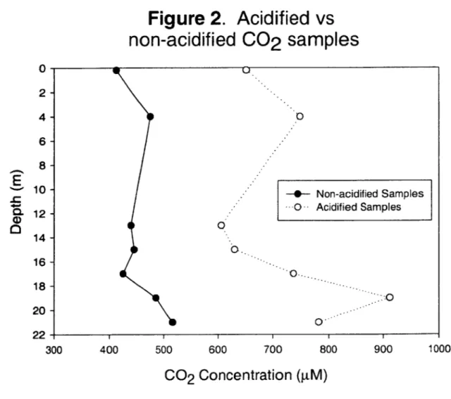
concentrations were determined using a headspace equilibration method, commonly used for measuring partial pressure of metabolic gases in water samples (Swinnerton et al., 1962; Kampbell and Vandegrift, S., 1998). Headspace equilibration was performed by documenting the water volume in each syringe, injecting a recorded volume of helium (He) into each syringe, and placing the syringes for 30 minutes on a wrist-action shaker to allow the water and headspace gases to equilibrate. Samples taken on and after October 1, 2004 were acidified with -25 pl of IN nitric acid to protonate bicarbonate ions, prior to He addition. A comparison of acidified versus non-acidified samples, collected on Oct 1, 2004 was used to correct previously analyzed CO2 data (Figure 2). The partioned headspace gases were then emptied into upper and lower sampling loops for injection onto columns having Molecular Sieve S and Hayspec C, respectively, as the packing material. Ultra-pure helium was used as the carrier gas, at a flow rate of 30 ml/min for the upper column and 18 ml/min for the lower column. CH4 and CO2 were detected by a thermal conductivity detector, and peak heights quantified by a Perkin Elmer Chart Recorder (Model PE056-1001). The lower column was used to separate

CO2 from other gases; CO2 follows the composite mixture to be recorded as the second peak (Figure 3). The upper column then resolves the composite mixture; the separated gases emerge and are recorded in the order 02, N2 and CH4(Figure 4). Standards were made in reusable 35 L gas cylinders using certified CH4 and CO2 in He. The standards mixed in the lab were tested against Scotty Transportable@ gases and replicate samples for CH4 and CO2 agreed within 2 percent and 7 percent, respectively (Figures 5 and 6). Peak heights for each gas were converted to partial pressures based on the standard

curves, Henry's law constant (Hemond and Fechner-Levy, E., 2000), water sample volume and headspace volume readings.

Figure 2. Acidified vs

non-acidified

C02

samples

.[

Co

Concentration (gM)

14-E

%_j

Figure 4.

60

Chromatogram of

Lower Column

40 -20 - 0--20 -0 20 40 60 80 100 120 140 160 180

Time (seconds)

E

-c

C02

Composite

Peak

Figure 4.

Chromatogram of Upper Column

I I I I I I 0 20 40 60 80 100 120 140 160 180

Time (seconds)

\2

N2

CH4

Figure 5.

CH

4

Standard Comparison

-I

CH

partial pressure (psi)

0 0 EC

as

Figure 6.

C02

Standard

Comparison

C02

Partial Pressure (psi)

12 10 -* Lab Standard o ScottyR) Standard 0

Ec

0-IV. CALCULATIONS

To quantify the redox balance in UML's hypolimnion, the 15-20 m depth interval was considered the control volume. The 15-20 m control volume was chosen for the mass balance calculations because: i) the depth was clearly within the zone of CO2 accumulation throughout the sampling period; ii) it was only necessary to consider diffusion across the 21 m surface (the other "boundaries" are the sediment-water interface); and iii) the most complete measurements were available for this region.

The masses of C0 2, CH4, NO3~, SO4

3

-and Fe2, in the hypolimnion of UML were calculated as follows. The concentrations of each substance were linearly interpolated between the sampled depths at 1 m intervals. The concentration of a substance in each I m thick stratum was determined as the average of the concentration at the top and bottom of that stratum. The area at depth was determined from multiple bathymetric maps to the same I m intervals as the limnological data. UML bathymetry data used for the mass balance calculations are presented in Table 2. The volume of each 1 m thick stratum was determined assuming that each stratum could be represented as an irregular cone (Wetzel and Likens, 2000). Finally, the mass of each substance in that stratum was determined as

Where Mass, is the mass contained in the hypolimnion (mmol m ) at the early sampling date, August 4, 2004 and Mass2 is the mass contained in the hypolimnion at the late

sampling date, November 22, 2004. D is the diffusive flux from the hypolimnion to the epilimnion. It was calculated using Fick's Law:

D = KiDC (2)

az

where K is the coefficient of vertical eddy diffusion andiL (mmol m4_{) is the}

az

concentration gradient of the substance of interest at the control volume surface. Based on temperature gradient estimates for UML determined by Senn (2001), a K = 0.02 0.01 cm2 _{s-I was used.}

Table 2. UML bathymetry data used for mass balance

calculations

Depth Area* Areat

M 10 5 m2 10 5 m2 0 5.83 5.00 3 4.19 3.57 6 3.67 3.09 9 3.19 2.70 12 2.7 2.30 15 2.06 1.74 18 1.62 1.39 21 1.2 1.04 24 0.7 0.52 Depth Interval Volume m 10 6 m2 15-16 1.85 16-17 1.75 17-18 1.65 18-19 1.5 19-20 1.35

* from Spliethoff, 1995 (Areas

t from Xanat Flores, personal countours)

determined by planimeter)

V. RESULTS

T, 02, pH and Conductivity Profiles

Temperature, dissolved oxygen, pH (Appendix B) and conductivity (Appendix B) measurements from 2004 were found to be consistent with previous UML studies

(Aurilio et al., 1994; Spliethoff et al., 1995; Senn 2001). A well-established thermocline was evident on the first sampling date on May 13, 2005, at which time some oxygen depletion was also evident (Figure 7 and 8). Oxygen consumption continued through June, and oxygen levels were below detection in the deepest 12 meters by late July (Figure 9). Summer dissolved oxygen profiles had a local dissolved oxygen minimum at the thermocline, a feature also observed in previous years (Aurilio et al., 1994). A depth of 8-10 m below the surface represented the base of the thermocline throughout the summer and early-fall, with a gradual thermocline deepening over the course of the fall. The water column remained stratified, with the bottom -8 meters unmixed, through the final sampling date of December 15, 2004. The pH measured above 8 in the epilimnion during the height of the summer, while hypolimnetic values ranged from 6.1 to 7.2. The average conductivity below 15 m was stable at 1.64 t 0.2 mS/s, while the epilimnion had an average value of 0.58 ± 0.09 mS/s from the surface to -11 m. There was a steep conductivity gradient at -12 m that remained stable until late November, when the chemocline began to deepen.

Figure 7. Temperature Profiles

*

4

-

6-

Temperature (0C)

Figure 8. Temperature Contour

Day during 2004 sampling period

day 147 = May 27, 2004

day 350 = Dec 15, 2004

Figure 8. Dissolved Oxygen Profiles

Dissolved Oxygen (mg/L)

8-9]

Y

C

Inorganic Nitrogen Profiles

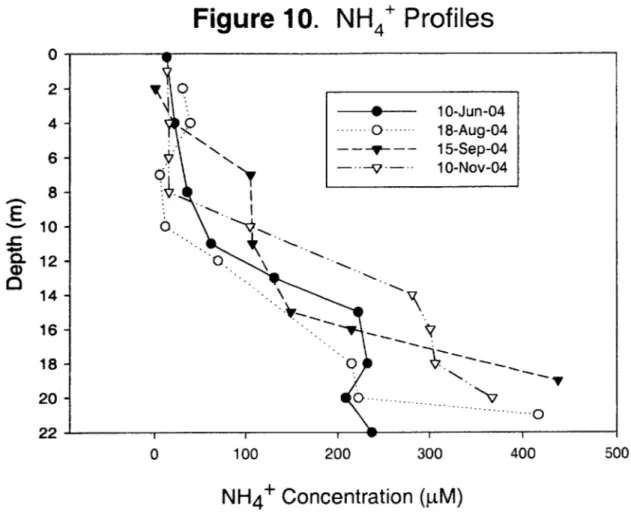
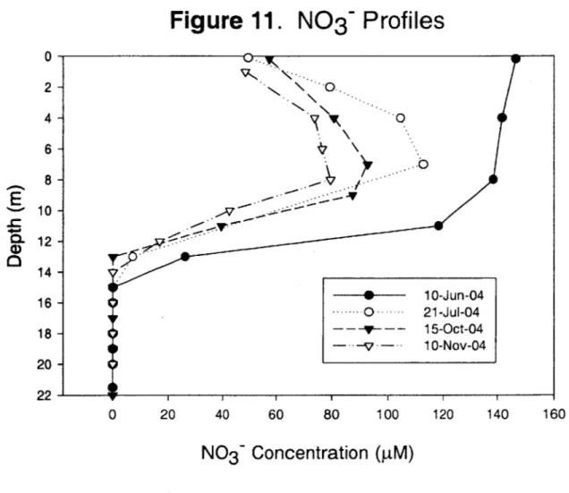
Nitrogen inputs (stormwater runoff, combined sewer overflows, and former industrial activities) occur along the Aberjona Watershed, resulting in elevated levels of ammonium (NH4*) and nitrate (NO~) in UML (Senn 2001). From the beginning of sampling, a mid-depth (7-11 m) peak in nitrate concentrations was apparent, with N0 3

levels frequently exceeding 100 pM. Deeper in the water column, nitrate disappeared and nitrate depletion in the hypolimnion was found from the onset of sampling. At the same time, NH4' was found in high concentrations in the hypolimnion, as high as 600 pM at the sediment surface. Figures 10 and 11 display NH4' and N0 3~ profiles from selected

sampling dates, Appendix B presents complete Nitrogen data. The elevated levels of NH4' in the hypolimnetic waters is most likely a result of NH4' diffusion from the

sediments where the breakdown and mineralization of organic matter (ammonification) is taking place (Kalff 2002). The NH4+ diffuses from the sediments, up through the water column, until it reaches the interface between oxic and anoxic waters (oxycline), where it is oxidized to NO3 (nitrification). The nitrification reaction,

NH4 +202 -+ N0 3~+ H20+ 2H+ (3) consumes ammonium and oxygen, while producing nitrate. The nitrification process is most likely responsible for the mid-depth peak of N03- and the DO minimum at the thermocline observed in UML. While equation (2) is a redox reaction and involves the transfer of electrons, the reaction occurs outside our control volume and therefore does not influence our mass balance. Furthermore, the absence of N0 3~ in the hypolimnion

Figure 10. NH

Profiles

NH

+

Concentration (pM)

0--v

Figure 11. N0

3

~

Profiles

N0

Concentration (pM)

Ec

v

Fe2+ Profiles

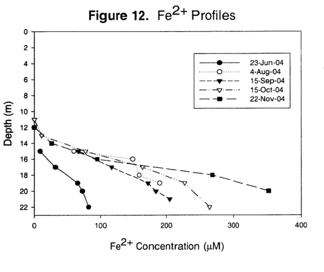
The presence of Fe2+, measured as acid soluble Iron(II), was found below a depth of 13 m and concentrations increased linearly towards the sediments (Figure 12). Overall Fe2

+ concentrations increased throughout the sampling period, reaching a maximum of

-350 ptM in late November. The accumulation of Fe2+ in the hypolimnion comes from

the oxidation of organic matter with the associated reduction of insoluble Fe3+ in the sediments. Insoluble Fe3+ oxides and oxyhydroxides settle onto the sediments and

become subject to reduction, producing Fe2+ once the DO, manganese (Mn 4), and nitrate have been utilized as electron acceptors during the decomposition of organic matter. Such conditions prevailed in UML since DO and nitrate were never present in the hypolimnia during the sampling period; therefore, the production and accumulation of Fe2+ is reasonable.

It should be noted that manganese was not measured during this study, but was found to be neglibible in UML by Senn 2001. In Senn's study of UML, acid-soluble manganese never exceeded concentrations of 20 p.M, even at the deepest depths, and at such low levels Mn can be considered negligible in terms of the electron budget.

Moreover, as an electron acceptor, Mn 4 _{provides more free energy and is preferentially}

Figure 12.

Fe2+

Profiles

Fe

+

Concentration (pM)

8-0-%,

S042 Profiles

Sulfate profiles (Figure 13) resemble nitrate profiles in that concentrations decrease through the hypolimnion as So42-is used as an electron acceptor in the

anaerobic decomposition of organic matter (Steenbergen et al., 1984). However, unlike N03~, the complete depletion of sulfate in the hypolimnia did not happen during the

sampling season. Hypolimnetic sulfate concentrations decreased linearly throughout the summer until Oct 1, 2004, when concentrations jumped back up to levels similar to the beginning of the summer and then decreased again. The cause of the sharp increase in sulfate concentrations is unknown. It is likely that reduced sulfides present in the samples could have oxidized during storage and added to the measured sulfate

concentrations. It is also possible that a storm event that occurred just prior to the Oct 1, 2004 sampling date brought in large amounts of cold, S042- rich (average -125 gM) water that underflowed into the hypolimnion (see Table 3 for storm data). Assuming this was the case, the storm event also brought in NO3 to the hypolimnion at an average concentration of 62 pM; such low concentrations did not affect the mass balance.

Alternatively, the N0 3~ brought in by the storm was most likely immediately reduced and therefore not observed in the nitrate profiles.

Figure 13.

_so

₄

2

_{- Profiles}

7

.--

'F-r''

S042-

Concentration (pM)

14-E

/

Table

3.

Late September 2004 Storm Data

Flow S042 NH4

NO3-Site Date Time (m3_{/s) (pM) (pM)}

(M) USGS* 9/28/2004 11:45 1.25 101.18 16.56 36.19 USGS* 9/28/2004 13:35 1.85 188.28 14.34 77.41 USGS* 9/28/2004 16:40 3.00 78.70 14.06 59.80 USGS* 9/28/2004 18:40 2.97 70.27 8.77 50.82 USGS* 9/29/2004 12:10 4.36 106.80 19.48 57.56 USGS* 9/30/2004 10:30 2.49 171.42 34.54 69.55 USGS* 10/1/2004 11:30 1.54 154.57 18.50 86.03

CH4 and CO2 Profiles

Dissolved methane distributions during the sampling period showed maximum concentrations at the sediments with a rapid decline towards a depth of -10 m. The process of methanogenesis occurs in the sediments, during which organic matter is fermented into methane and carbon dioxide. Methane concentrations continued to increase throughout the sampling period and maximum concentrations of dissolved methane (705 ptM) occurred on November 22, 2004. Concentrations in the epilimnion were always <1 [tM. Figure 14 presents methane profiles from selected dates.

Due to atmospheric exchange, the epilimnion maintains a constant amount of

CO2. At the surface, the average CO2 concentration was -650 ptM, which is about twice

the amount expected if the surface water (using recorded pH data, Appendix B) were in equilibration with the atmosphere. The surface concentration was constant through the water column until -10 m where it increased through the hypolimnion (Figure 15). The large amount of CO2 in the hypolimnion is a result of the net decomposition of organic

Figure 14.

CH

4

Profiles

CH

Concentration ( M)

Figure 15.

C02

Profiles

CO

Concentration (gM)

a)

I

-j

Rates of decomposition and reduction of electron acceptors

Changes in masses of CO2 and CH4 were linear with time indicating that the rate of decomposition of organic matter was constant throughout the measurement period (4-Aug-04 to 22-Nov-04; Figure 16). Similarly, changes in masses of the electron acceptors were also linear, except for S042- as mentioned above (Figure 17). In the case of SO42 the rate of reduction was calculated for more than one time period (4-Aug-04 to 15-Sep-04 and 16-Sep-15-Sep-04 to 22-Nov-15-Sep-04). For the whole sampling period, molar quantities of methane and carbon dioxide changed the most, followed by sulfate and then iron (Table 4). Neither nitrate nor 02 changed because measurements began after anoxia and nitrate depletion were established in UML.

The overall hypolimnetic decomposition rate, measured as CO₂ accumulation, was determined to be 7.5 ± 0.37 mmol CO₂ m-2 d-. Unfortunately, there are no previous estimates of decomposition in UML to compare this value to. The hypolimnetic CO2 accumulation rates determined by other studies are summarized in Table 5. Values in the range of 4.7 to 10.7 mmol CO2 m-2 d-, based on observations in other systems using similar hypolimnetic fractions, suggest that the model used here provides a reasonable rate estimate of organic matter decomposition in UML.

Figurel6. Change in hypolimnetic mass

of

C02, CH

4

during 110 day sampling period

14 12 - 10- 8- 6- 4- 20

-4-Aug 18-Aug 1-Sep 1-Oct 15-Oct 27-Oct 10-Nov 22-Nov

2004 Sampling Dates CJ 0 E E 0 C02 0 0

_CH4

Figure 17. Change in hypolimnetic mass of 02, N03~, Fe

₊

_and

SO

-

during 110 day sampling period

120 100-80 Fe2+ E 75 60 -E E v 40-20

02, N03

So

4-Aug 18-Aug 1-Sep 1-Oct 15-Oct 27-Oct 10-Nov 22-Nov

Table 4.

Rates of change of hypolimnetic species

Molar

Species

Interval

quantities

(no. of days) mmolem-2d-1

02 N0 _3~ Fe2+ So 2 S0 2 CH₄ Co 2 4 Aug - 22 Nov (110) 4 Aug - 22 Nov (110) 4 Aug - 22 Nov (110) 4 Aug - 15 Sep (42) 16 Sep - 22 Nov (68) 4 Aug - 22 Nov (110) 4 Aug - 22 Nov (110) 0 0 +0.36 -1.35 -0.71 +1.99 +7.54 0.03 0.09 0.08 0.11 0.37

Table

5.

Comparison of

CO

accumulation in other

lakes

Mattson & Likens (1993) Schafran &Driscoll (1997) This Study

Uncertainty in rate estimates

Uncertainty estimates for the rates of decomposition and reduction of electron acceptors were calculated for the accumulation and diffusive flux terms. Accumulation uncertainty was determined by,

I (V ± 10%)i - ([S] ± 10%) (5)

where i represents a stratum within the 15-20 m control volume (i.e. 15-16 m for the 15 m slice of the control volume) and V is the stratum volume, estimated from a best fit curve to UML bathymetric data with an associated uncertainty of ±10%. The term, S, is a particular redox species concentration averaged from the top and bottom of that stratum. The analytical uncertainty in any laboratory measurement for a species concentration was determined using the method described by Miller and Miller (1984). All the standards measured during the experiment were used to construct a linear calibration curve. The standard deviation for the substance concentration was then calculated by EXCEL or SigmaStat statistical software and confidence limits for any measurement were calculated using a t value with n-2 degrees of freedom.

The turbulent diffusion term has an uncertainty calculated by

(K, ± 50%) * (d[S]/dzavg-,5m ± s.d.) * (Ai5m ± 10%) * At. (6) No uncertainty was used for the sampling period, At, because the maximum possible uncertainty (<12 hours = ±3%) was insignificant relative to other errors. AI5m is the lake area at 15 m, which is equal to 1.85 x 105 m2 + 10%. The term d[S]/dzavg-15m ± s.d. is the average gradient over the sampling period at 15 m ± the standard deviation of the

(2001), was used as 0.02 cm2 s ± 0.01 (i.e. ±50%) and is the majority of the uncertainty. Total uncertainty for rates were calculated by standard methods of error propagation

(Peters et al., 1974; Harris 1998).

Electron budget

The reducing equivalents were calculated based on the electrons necessary to reduce the molar quantities of electron acceptors. In the case of Fe2+ production I eq is used per mol Fe produced. That is, one electron is needed to reduce Fe3+ to Fe2_+.

Likewise, 8 electron equivalents are needed for sulfate reduction and methanogenesis. Therefore, the data in Table 6 represents an estimate of the electron flow through the anaerobic processes in the hypolimnion. The results of Table 6 indicate that the hypolimnetic electron budget was not balanced during the sampling period; the rate of

CO2 accumulation exceeded the combined rates of reduction of the electron acceptors.

The electron balance showed an excess of 21 percent organic matter decomposition that was unexplained.

Table 6. Reducing equivalents necessary to reduce the

molar quantities of electron acceptors

Molar quantities mmol*m-2_-d~' 0.36 -0.96 1.99 7.54 Reducing equivalents mmol e-mO-2-d'1 0.36 7.66 15.95 30.16 Species Fe2+ SO 42 -CH₄ Co 2 Molar quantities mmolem-2 39.13 -105.27 219.33 829.50

Carbon Flow

The contribution of each electron acceptor to carbon flow (i.e. the complete breakdown of organic compounds to CO2 and CH4) is presented in Table 7. The associated carbon equivalents were estimated by assuming that the organic substrate contained the Redfield ratio of elements (i.e. glucose) and that it decomposed according to the stochiometry shown in Table 1. In terms of carbon flow, methanogenesis was the predominant process, accounting for 53 percent of total organic matter decomposition during the sampling period. Sulfate reduction was the next most prevalent (25%) and then followed by iron, which accounted for 0.4 percent of total decomposition in UML.

Table 7. Carbon equivalents produced during the

reduction of electron acceptors

Molar Species quantities mmolem-2 Fe2+ 39 ±3.3 So 42- 105 ±10 CH4 219 ±12 CO2 equivalents Mmol Cem-2 3.3 0.8 210 20 439 24 % of CO2 accumulation 0.40 25.32 52.92 Excess CO2 % 21.36

VI. DISCUSSION

Comparison to other lakes

There are other studies that have done relatively similar hypolimnetic budgets for redox active chemical species (Ingvorsen et al., 1982; Schafran and Driscoll, 1987; Kelly et al., 1988; Mattson and Likens, 1993). All of these studies used stoichiometric

equations for the electron acceptors, analogous to those presented in Table 1, and carbohydrate type carbon as the carbon substrate. The overall electron budgets for the

lakes examined in these studies varied from a 60 percent excess of electron acceptors in Lake 226N, Ontario, to a 37 percent excess of CO2 in Mirror Lake, New Hampshire. The

compiled data is summarized in Table 8.

The Canadian experimental lakes studied by Kelly et al. (1988) have little 02 present in the hypolimnion and are therefore most comparable to UML. Like UML, the experimental lakes have the highest percentage of decomposition attributed to methane production; sulfate reduction also appears to be higher. Nitrate reduction is variable, but rather low, and iron reduction appears to be negligible in the CO2 accumulation of the

Table 8. Comparison of overall electron budget from

several lakes

Lake Excess Reference

C0 2 %

L226N -60 Kelly et al. (1988)

L227 -6 Kelly et al. (1988)

L223 11 Kelly et al. (1988)

Mirror 37 Mattson & Likens (1993) Dart's 0 Schafran &Driscoll (1997)

Table 9. Comparison of electron acceptors as percent of

CO

accumulation to the Canadian experimental lakes

S042 N03 CH4 acceptor as percent of CO2 25 13 71 30 1 68 30 1 42 25 0 Fe Total accumulation 3 160 2 106 6 88 53 0.4 Reference Kelly et al. (1988) Kelly et al. (1988) Kelly et al. (1988) 79 This study Lake L226N L227 L223 UML 02 Electron 47 5.5 9 0

Possible explanations for the electron imbalance

Possible explanations for the electron imbalance in UML fall into three

categories: (1) calculation errors including analytical errors and errors in stoichiometry; (2) underestimation of iron reduction; and (3) underestimation of methane

Analytical errors were 10 percent or less for all the measured species. Even with an uncertainty of 20 percent, such analytical error is not likely to change the results of this study.

The overall stoichiometric ratios for the equations in Table 1 depend on the oxidation state of the carbon substrate. For example, the anaerobic degradation of

cellulose theoretically yields equimolar amounts of CH4 and CO2. If the carbon substrate was more reduced than carbohydrate, for instance a long-chain fatty acid, decomposition will yield a CH4:CO2 ratio greater than 1. Therefore, the amount of carbon flow during methanogenesis and other processes of organic matter mineralization depend on the chemical composition of the organic matter undergoing decomposition. The

stoichiometric assumptions (Table 1) used in this study and by others (Kelly et al., 1988; Mattson and Likens, 1993) tend to overestimate the reduction rates. Correcting the equations using a carbon substrate with a lower oxidation state could lead to the reverse problem, a deficit of CO2 with respect to that expected.

The rate of iron reduction may be underestimated by the method of measuring dissolved Fe accumulation. It is likely that a certain amount of Fe precipitates as FeS or FeS2 minerals and is therefore being neglected in the budget. When anoxic conditions develop, Fe2+ that is produced can precipitate as FeS or FeS2, in the presence of enough

of iron reduction, any iron reduction that resulted in FeS precipitation was neglected. In an attempt to correct for this problem, FeS formation was estimated by assuming: (1) that all of the reduced sulfate resulted in FeS formation and (2) that on a molar basis 30 percent of sulfate reduction resulted in formation of FeS (based on work by Rudd et al.,

1986). Rudd et al. (1986) determined that an average of about one-third of the

endproducts of sulfate reduction were iron sulfides which trap the iron in the sediments. After making these adjustments the excess CO2 was reduced from 21 percent to 19 percent for the first case and to 20 percent excess CO2 in the second. All in all, even maximum possible FeS formation does not explain the excess CO2 accumulation in the hypolimnia of UML and concludes that iron reduction is small in terms of the total decomposition in UML.

There is also the possibility that methane production was underestimated and could account for the excess CO2. Methane could have escaped from the sediments via ebullition and was therefore not measured by methane accumulation in the hypolimnion. Methane bubbles can form when the production of CH4 within the sediments exceeds the rate of its removal. Consequently, the total gas pressures within the sediments exceeds the hydrostatic pressure; supersaturation and thus bubble formation occurs (Rudd and Taylor, 1980). Methane lost from the sediments by ebullition is lost from the aquatic environment entirely. By this way, the ecosystem loses energy, carbon and reducing

1980; Mattson et al., 1993). To account for the excess C02 measured in this study, 0.78 mmol m-2 d- CH4 would have been lost from the hypolimnion via ebullition, or 28 percent of the total CH4 produced.

Finally, the underestimation of methane production and thus the budget

discrepancy could be explained by the storage of methane (or another reduced product) in the sediments. The excess CO2 accumulated at an average rate of about 1.6 mmol m-2 d-in UML throughout the sampld-ing period. This rate of excess CO2 accumulation could be explained by the accumulation of a reduced end product with a volume-weighted

concentration of 35 pM (expressed as CO2 equivalents) over a 110-day period. For example, if 4 liters of methane (at 0* C and 1 atmosphere pressure) were stored per m2 _of sediment in a 110-day period this would account for 100 percent of the excess CO2. It is possible for methane to be stored in the sediments and diffuse out and be oxidized at other times of the year (Rudd and Hamilton, 1978).

VII. CONCLUSION

Decomposition of organic matter, measured by the accumulation rate of C0 2, was measured in the hypolimnion of UML. Rates of reduction of anoxic terminal electron acceptors were calculated but could not account for the decomposition of organic matter. During the period of this study approximately 80 percent of the decomposition in the hypolimnion of UML could be accounted for, while 20 percent remains unexplained. Several possibilities to explain the excess decomposition have been considered. The most likely possibility includes the underestimation of methane due to ebullition and/or the storage of gaseous methane in the sediments. Future studies in UML should include measurements of methane ebullition rates and iron sulfide particulates. Another useful measurement would be to determine the C:H:O ratio of organic matter in UML.

VIII. Appendix A

One of the main objectives of any water monitoring program involving fieldwork is the assurance of high quality, reliable data. In fact, the success of a water monitoring program can often depend on the sampling procedure adopted, regardless of how

sophisticated the analytical approach may be. Unfortunately, sampling procedures have been neglected in recent years, while advancing analytical technology has been the focus (Broenkow 1969). It is important that an equal amount of effort should be directed towards improving and updating sampling methodology. This is particularly true for dissolved gases in hypolimnia of lakes since significant temperature and pressure changes can occur as the sample is lifted to the surface, as well as gas exchange with the

atmosphere. The traditional method for sampling dissolved gases from the hypolimnion uses tubing and a peristaltic pump to fill glass BOD bottles at the surface. Such a method is not suitable for dissolved gases and introduces the possibility of all the problems

mentioned above.

The problem of sampling dissolved gases from hypolimnia of lakes without outside influences (i.e. temperature changes, pressure changes and atmospheric contamination) required a portable sampler that could be used to obtain samples at precise depth intervals over the water column. The sampler described below was designed specifically to fit this need, but also allows samples to be analyzed by

half, were cemented at each end and spaced apart to secure the lip of a 50 ml syringe in place. The syringes are held in place by the reducer bushings but can easily be attached or removed.

Before the syringes are attached to the PVC frame for sampling, the -30 m tubing used to collect water samples for the other redox species is completely filled with water. Once this is done, the sampling syringe and the motor syringe (see Figure A-I and A-2), which is completely filled with - 50 ml water, can be placed in the PVC frame. The

motor syringe is then attached to one end of the tubing and the surface syringe (with no water) is attached to the other end of the tubing using tubing connectors. Because the motor syringe is filled with water, the plunger is fully extended and reaches the plunger end of the sampling syringe. The two plunger ends are connected using two Keck clamps; a Keck clamp happens to perfectly fit around the lip of a 50 ml syringe plunger. When the sampler is fully loaded and ready to lower over the side of the boat, the sampler is tied by a rope to the Hydrolab which serves as both a weight and depth meter.

As the sampler is lowered over the side of the boat, the 3-way Luer lok® valve on the sampler syringe is opened under water to eliminate air filling the valve. Once the sampler is lowered to the measuring depth, the 3-way Luer ok® valve on the surface syringe is opened. The plunger on the surface syringe is pulled and water from the tubing fills the surface syringe. As this is happening, the plunger on the motor syringe closes as water from the motor syringe replaces the water pulled from the tubing. Furthermore, since the motor and sampling syringes are connected end-to-end, the closing of the motor syringe plunger causes the sampling syringe plunger to open and fills the sampling

syringe with water. The amount of water pulled into the surface syringe is equal to the amount of water collected in the sampler syringe.

During sampling, the sampling syringe is flushed with water three times and is done so by simply pulling and closing the plunger of the surface syringe. After the desired sample volume is collected in the sampling syringe, the sampler and hydrolab are lifted to the surface and the 3-way Luer lok® valve on the sampling syringe is closed and capped underwater to avoid contact with the atmosphere. The sampling syringe is then removed from the PVC frame and immediately placed in a bucket of ice water. A new sampling syringe is placed into the PVC frame and the sampler is ready to be lowered to collect another sample.

It is important for the sample-filled syringes to be kept in cold water to avoid changes in sampling depth temperature and pressure. The ice water bucket used in this study was equipped with a "dock" of PVC reducer bushings cemented together (Figure A-3). This allowed the syringes to securely stand in the bucket with plunger up and not hit each other during transport.

Figure A-4 shows the water column profile of replicate samples of CO2 taken on

September 1, 2004. The replicate samples were on average within 6 percent of each other, indicating that the analytical method as well as sampling method used in this study afforded reliable dissolved gas data.

is estimated to be $30.00, but most of the parts can be found around the lab and would not have to be purchased.

Figure A-1. The Dissolved Gas Sampler Diagram

\AXter-filled pub:ng thit cornects 7o t'e "ua-ace

~ moctor synn~ge~

Keck Clamp -:1.ge Connector

Table A-1. Cost and parts list for sampler

Part #/ sampler Cost

Tubing Connectors (1/8" Tubing) 3-way Luer lok valve

Tie wraps (6") Reducer Bushings (1.5" x 3/4" Slip) PVC pipe (1.5") Keck Clamp Misc. hardware

PVC primer and cement Rope 3 3 2 8 1.47 ft 2 14.77/20 42.60/25 30.10/1000 0.95 1.11 /ft 24.00/6 Total: Cost/sampler $2.21 $5.11 $0.06 $7.60 $1.63 $8.00 $5.50 $30.00

IX.

Appendix B

Summary of Limnological Data

The hydrolab data and chemical species concentration profiles from the water column of the Upper Mystic Lake are tabulated on the following pages.

Table B-1. 13-May-04 Profile

Table B-2. 27-May-04 Profile

Depth Temp Cond DO pH ORP NH4+ N03

(M) (0C) (mS/cm) (mg/L) (mV) (pM) (PM) 0 16.63 0.71 8.44 7.47 548 1 16.60 0.71 8.43 7.49 533 20.01 108.98 2 16.53 0.71 8.43 7.50 529 3 16.44 0.71 8.32 7.50 524 13.31 73.58 4 15.93 0.67 8.10 7.47 514 5 13.69 0.70 6.77 7.24 506 24.92 89.07 6 10.14 0.71 6.89 7.15 497 7 7.90 0.75 7.40 7.09 467 43.32 108.98 8 6.73 0.78 7.56 7.06 415 9 6.00 0.81 7.58 7.06 359 10 5.61 0.86 6.77 7.04 332 55.01 100.13 11 5.28 0.91 6.00 7.04 309 12 4.79 1.04 4.45 7.03 294 82.55 75.79 13 4.21 1.30 0.68 7.01 265 14 3.85 1.46 0.45 7.03 225 119.72 40.39 15 3.63 1.53 0.37 7.03 211 16 3.45 1.59 0.33 7.03 201 18 3.32 1.68 0.29 7.03 181 20 3.32 1.69 0.27 7.05 174 22 3.35 1.53 0.26 7.08 166 24 3.36 1.50 0.26 7.19 157

Table B-3

10-Jun-04 Profile

Depth Temp DO pH ORP NH4* N03

(M) ("C) (mg/L) (mV) (AM) (AM) 0.2 20.77 8.85 5.58 549 13.56 146.11 1 21.36 9.38 6.1 532 2 21.68 9.32 7 486 3 20.6 9.41 6.9 497 4 20.54 8.92 6.83 504 22.67 141.45 5 20.3 7.81 6.78 508 6 18 5.75 6.35 519 7 16.41 5.15 6.19 524 8 14.64 4.99 6.06 527 36.39 138.33 9 8.05 6.83 5.61 533 10 7 6.9 6.5 510 11 5.69 4.94 6.9 456 61.92 118.10 12 5.09 3.22 6.91 337 13 4.6 0.8 6.91 314 131.23 26.26 14 4.2 0.26 6.87 171 15 3.93 0.23 6.86 154 221.39 0.00 16 3.74 0.24 6.86 152 . 17 3.51 0.24 6.85 148 18 3.39 0.24 6.9 137 231.99 0.00 19 3.39 0.26 6.9 134 20 3.39 0.24 6.91 130 208.20 0.00 21 3.38 0.22 6.92 125 1 22 3.39 0.22 6.98 121 237.14 0.00

Table B-4. 23-Jun-04 Profile

Depth Temp Cond DO pH ORP Fe2+ NH4+ NO0

(M) (C) (mS/cm) (mg/L) (mV) (PM) (pM) (pM) 0.2 22.01 0.72 8.2 7.54 513 10.84 144.56 1 22.01 0.72 8.34 7.68 514 2 21.94 0.72 8.39 7.71 514 11.07 138.33 3 21.89 0.72 8.15 7.73 510 4 20.45 0.71 7.83 7.47 509 29.64 138.33 5 15.22 0.71 5.42 7.1 510 6 12.35 0.73 4.83 6.87 510 7 8.76 0.77 4.95 6.77 500 29.85 132.11 8 7.37 0.80 4.87 6.65 430 9 6.29 0.84 4.31 6.62 371 10 5.81 0.89 3.57 6.63 329 11 5.33 0.96 2.96 6.67 319 12 4.63 1.19 1.2 6.7 295 13 4.16 1.42 0.36 6.78 267 144.87 4.47 14 3.88 1.53 0.26 6.79 245 15 3.71 1.59 0.25 6.79 240 8.20 214.27 0.00 16 3.59 1.63 0.23 6.79 230 17 3.47 1.68 0.22 6.79 224 31.48 212.90 0.00 18 3.41 1.73 0.21 6.8 213 19 3.4 1.74 0.22 6.83 210 64.81 233.36 0.00 20 3.38 1.75 0.19 6.85 193 71.76 253.66 0.00 21 3.39 1.75 0.18 6.87 186 _ 22 3.4 1.75 0.19 6.89 184 80.77 246.31 0.00

Table B-5. 7-Jul-04 Profile

Depth Temp Cond DO pH ORP Fe2

+ NH4+ NO3 (M) (0C) (mS/cm) (mg/L) (mV) (pM) (pM) (pM) 0.2 24.75 0.72 8.37 7.74 390 1 24.66 0.72 8.4 7.78 389 2 24.5 0.72 8.42 7.79 389 10.93 79.12 3 24.47 0.71 8.35 7.8 389 4 21.05 0.71 7.42 7.32 384 9.82 81.65 5 16.34 0.72 5.63 6.96 365 6 11.24 0.76 3.3 6.65 321 7 8.76 0.79 3.23 6.43 267 20.93 75.32 8 7.25 0.82 3.3 6.41 235 9 6.18 0.87 2.44 6.38 211 10 5.73 0.92 1.52 6.39 198 11 5.14 1.02 1.12 6.43 175 12 4.76 1.14 0.54 6.44 158 13 4.2 1.43 0.38 6.49 142 141.01 8.22 14 4.04 1.50 0.54 6.53 51 15 3.8 1.59 0.43 6.52 37 54.84 148.71 8.22 16 3.57 1.67 0.32 6.57 19 17 3.48 1.73 0.34 6.58 14 54.03 160.77 0.00 18 3.45 1.74 0.52 6.63 36 19 3.44 1.76 0.45 6.63 29 53.25 157.39 0.00 20 3.46 1.77 0.4 6.65 23 21 3.46 1.78 0.37 6.68 17 107.49 188.54 0.00