Open Archive TOULOUSE Archive Ouverte (OATAO)
OATAO is an open access repository that collects the work of Toulouse researchers and makes it freely available over the web where possible.This is an author-deposited version published in : http://oatao.univ-toulouse.fr/
Eprints ID : 18828
The contribution was presented at CM 2016/MFPT 2016 :
http://www.bindt.org/events/CM-2016-and-MFPT-2016/
To cite this version : Salameh, Farah and Picot, Antoine and Chabert, Marie and Maussion, Pascal Hybrid parametric/non-parametric models for lifespan modeling of insulation materials. (2017) In: 13th International Conference on Condition Monitoring and Machinery Failure Prevention Technologies (CM 2016/MFPT 2016), 10 October 2016 - 12 October 2016 (Charenton-le-Pont, France).
Any correspondence concerning this service should be sent to the repository administrator: [email protected]
Hybrid parametric/non-parametric models for lifespan modeling of
insulation materials
Farah Salameh, Antoine Picot and Pascal Maussion University of Toulouse, LAPLACE, INPT-ENSEEIHT
31071 Toulouse, France Marie Chabert,
University of Toulouse, IRIT, INPT-ENSEEIHT 31071 Toulouse, France
+33 (0)5 34 32 22 25 [email protected] Abstract
This paper considers the modelling of insulation material lifespan. This problem is crucial in electrical engineering, and specially for aircraft reliability, since about 40% of electrical machine failures stem from insulation. According to the material physical properties and to the sightings reported in the literature, the proposed model should relate the logarithm of the insulation lifespan to the logarithm of the electrical stress factors (voltage and frequency) and to the temperature. The possible interactions between these three predominant aging factors must also be considered. Moreover, due to a constraint of low experimental cost, the number and configuration of experiments should be optimized through a design method. Parametric modelling through multilinear regression requires the estimation of a potentially high number of parameters in view of the reduced data set. The method proposed in this paper thus combines parametric (multilinear regression) and non-parametric (regression trees) approaches through so-called hybrid models. First, a regression tree automatically classifies the experiments into ranges corresponding to relevant operating modes. Second, a multilinear model is associated to each leaf of the tree. This approach brings a better understanding of the aging phenomena through the hierarchical organization of the factors and also provides simple, specific and thus effective multilinear models in each lifespan range. The method performance is analysed through real data: training and test sets correspond to experiments on twisted pairs covered by an insulating varnish. The proposed method shows improved performance with respect to multilinear regression on one hand and to regression trees on the other hand.
1. Introduction
In the electrical engineering field, most critical applications, such as urban transports, aeronautics, or space, are moving towards more electric systems. Such systems offer significant benefits in terms of performance, impact on environment, and operating costs [1] but they also require higher electrical power than traditional systems [2]. Unfortunately, higher voltages and higher frequencies increase the risk of degradation in the electrical insulation [3]-[5] through Partial Discharges (PD) mainly. Given that around 40% of electrical machine failures result from insulation failures [5], [6], characterizing the lifespan of insulation materials under these new operating conditions
2 becomes crucial for the assessment of the global system reliability. In addition to electrical stress, insulation materials are subject to thermal, mechanical and environmental stresses acting simultaneously [7], [8]. Several models have been proposed to describe the effects of these different stresses on the insulation lifespan [7], [9], [10]. However, these models take into account a single stress factor (like the temperature in Arrhenius law or the voltage in the inverse power law) or at most two factors (mainly the electrothermal stress) at a time. Moreover, they are specifically designed for particular materials and their validity is assessed on very restricted factor ranges. Finally, they do not include the synergetic effects due to interactions between factors. In real-life, insulation materials are subject to a wide variety of operational and environmental stresses, thus independently studying the effect of each factor on the material lifespan is far too simplistic.
In this paper, a statistical approach for the insulation lifespan modeling is proposed. The twofold objective is to provide a reliable lifespan model with a minimum experimental cost. To comply with both the accuracy and the economical constraints, the number of experiments and their configuration are specified according to two experimental optimization methods: the Design of Experiments (DoE) [11] and the Response Surface (RS) [12], [13]. The proposed insulation lifespan models include three different stress factors: voltage, frequency and temperature, as they were identified as the predominant factors causing PD [3]-[5]. The effect of the three stress factors and of their interactions may be studied through classical multi-linear parametric models or with piecewise constant non-parametric models such as regression trees. This paper proposes an alternative approach: the effects are examined through piecewise linear models. These so-called hybrid models combine the classification of the experiments in different ranges of the stress factors according to their individual and combined effects on the lifespan and the multilinear parametric modelling of the lifespan on these identified ranges.
2. Problem statement and experimental set-up
2.1 Studied insulating materialThis paper presents results obtained for a 200°C thermal class insulating material widely used for electric machine wiring insulation. Note that the conclusions drawn in this paper have been confirmed by a second measurement campaign on a different insulating material of 220°C thermal class. The insulating material studied in this paper is composed of two insulating layers of Poly-Ether-Imide (PEI) and Poly-Amide-Imide (PAI). The studied samples are twisted pairs of 0.5mm diameter copper wires covered with this insulating material. Twisted pairs (Fig. 1a) were manufactured according to [14] as shown in Fig. 1b.
Fig. 1b. Manufacturing process of twisted pairs from copper wires
3 Fig. 1a. A twisted pair as a test sample
2.2 Considered stress factors
This study focusses on insulation aging caused by PD. The authors of [3]-[5] point out that electrical and thermal stresses are the predominant factors causing PD in electrical insulation. Therefore, three aging factors are considered in our study: the applied voltage (the amplitude V of a square wave voltage), its frequency F and the ambient temperature T. According to [10], the lifespan logarithm, Log(L), follows a multilinear model depending on Log(10V), Log(F) and exp(-bT), with b = 4.825u10-3. In order to get achievable lifespan measurements, the material is tested under higher-than-nominal stress levels ensuring PD regime. Temperature covers a wide range of operating conditions, realistic for an embedded electrical machine, but does not exceed the material thermal class. Table I lists the factors and specifies their ranges. Test samples are disposed in a climatic chamber where the temperature can be tuned to the desired value. A power electronic system generates a square voltage controlled in amplitude and in frequency. The lifespan of a test sample is defined as the failure time at which a short circuit occurs in the twisted pair. The experimental setup is displayed on Fig. 2. 30 experiments were carried out. Among them, 18 were specified according to a classical design method described in section 3, while the others have random values for V, F and T. For each experimental configuration, 6 twisted pairs were tested simultaneously.
TABLEI
STRESS FACTOR RANGES
Factor Min.
Value Max. Value
V 1 kV 3 kV
F 5 kHz 15 kHz
T -55°C 180°C Fig. 2. Test bench: climatic chamber and power electronics
3 Theroretical background: parametric and non-parametric lifespan
models
The classical approach to evaluate the effects of the factors and their interactions consists in computing a full parametric model. In the following, first and secondorder parametric models with interaction terms are developed. As previously stated, in order to reduce the experimental cost while ensuring the best model accuracy, experiments composing the model training set are specified according to two optimization methods: DoE for first order models and RS for second order models. The remaining random experiments are then used to test the model accuracy.
3.1 Parametric models from design optimization methods
3.1.1 Principle
4 data sets required for lifespan model estimation are restricted due to various experimental constraints: cost of tested materials, cost and availability of the test bench, limited experimental time, etc. Therefore, the number and the configuration of experiments needed to compute a full parametric lifespan model must be optimized to minimize experimental cost while ensuring the best model accuracy.
The most efficient method to evaluate the effects of several factors and their interactions on a response variable is the basic Design of Experiment (DoE) [11]. This method consists in assigning only 2 levels (normalized to r1) to each factor. Therefore, 2k experiments are needed to compute a parametric model including k factors and all their possible interactions. Each configuration is one of the 2k combinations between the two
levels of the k factors. The obtained design is then called 2k Full Factorial Design (FFD2) having an orthogonal experimental matrix [11] that provides the best statistical properties of the model in terms of coefficient accuracy [11]. With 3 factors, 8 experiments are required and the DoE lifespan model can be written as (1):
Log(L)DoE = M + EVXV + EFXF + ETXT + IVFXVXF + IVTXVXT + IFTXFXT +
IVFTXVXFXT (1)
where L is the lifespan (in (s)), XV, XF and XT are the three factor levels corresponding to
the values of Log(V), Log(F) and exp(-bT). M is the model constant, EV, EF and ET are the
three factor effects, IVF, IVT, IFT and IVFT are the different interaction effects. Model (1) is
a first order model with interaction terms. However, it may be of interest, for a better approximation of the lifespan model, to include quadratic terms of the main factors. The appropriate optimization method for second order models with interactions is the Response Surface (RS) method [12] [13]. RS lifespan model can be written as (2):
Log(L)RS = M + EVXV + EFXF + ETXT + IVV(XV)2 + IFF(XF)2 + ITT(XT)2 +
IVFXVXF + IVTXVXT + IFTXFXT (2)
where IVV, IFF and ITT are the quadratic effects of the factors.
The estimation of the quadratic term factors requires additional experimental points and thus additional factor levels with respect to DoE. According to [13], it is impossible to achieve the orthogonal experimental matrix property for second order designs. However, orthogonality can be obtained if the experimental matrix is excluded from the constant term. The design is then called “almost orthogonal”. There are two popular almost orthogonal RS designs for the second order models with interaction terms [13]:
x 3.3k Full Factorial Designs (FFD3): The number of required experiments is 3k.(three levels for each factor). The design is almost orthogonal if the three
levels are –1, 0 and +1 [13].
x Central Composite Designs (CCD): a CCD requires less experimental points than a full 3k design. However, five levels of each factor are needed instead of three. A CCD is composed of [12], [13]: a complete 2k DoE design, two axial
points on the axis of each factor at a distance T from the design center, defining two extra levels (rT), N0 central points at the design center. An almost
orthogonal CCD is obtained if [12], [13]:
2k(2k + 2k + N0) = (2T2 + 2k)2 (3)
Organized experiments were specified according to a CCD. The CCD is composed of the 8 experiments of the 23 FFD, 4 central points and 6 axial points with T = 2 to satisfy
5 represented in Fig. 3. Factors levels are given in Table II for organized experiments. Note that random experiments have factor levels belonging to the respective factor domains given in Table I. Models (1) and (2) have the general form of multi-linear regression models relating a response Y = Log(L) to the explanatory variables. Therefore, model coefficients can be estimated by the Ordinary Least Square (OLS) method [15].
TABLEII
STRESS FACTORS LEVELS
Level Log(10V - kV)
Log(F -
kHz) exp(–bT - °C)
–2 Log(10*1) Log(5) exp(55b)
–1 Log(10*1.174) Log(5.872) exp(34.82b) 0 Log(10*1.73) Log(8.7) exp(–26.12b) +1 Log(10*2.554) Log(12.77) exp(–119.74b) +2 Log(10*3) Log(15) exp(–180b)
3.1.2 Model Prediction Performance
The validity of parametric DoE and RS models in the factor domains given in Table I can be checked by applying them to the test set composed by the randomly configured experiments. The prediction performance of the models can be evaluated by comparing the predicted and measured values of Y and L through relative errors
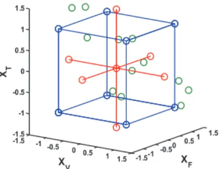
-1.5 -1 -0.5 0 0.5 1 1.5 -1.5-1 -0.50 0.51 1.5 -1.5 -1 -0.5 0 0.5 1 1.5 X F X V XT
Fig. 3 3D representation of factor levels
For each experiment we have performed 6 measurements of the lifespan logarithms (Ymeas). The set of Ymeas corresponding to the same experiment can be averaged leading to
Yav and a 95% Confidence Interval (CI) of Yav can be computed by assuming a normal
distribution of the set of repeated Ymeas. This CI represents the variability of the measured
lifespan logarithms in each experiment. The evaluation criteria of the model prediction performance on the test set are:
- Relative errors between predicted and measured average Log(L): REY = 100u_Yav – Ypred_/Yav
(4)
- Relative errors between measured average L in the original scale (Lav) and predicted
L (Lpred) obtained by applying the logarithmic back transformation on Ypred:
6 REL = 100u_Lav – Lpred_/Lav
3.1.3 Parametric Lifespan Models
The first order lifespan model with interactions has the form of (1) where L is in (s). It is estimated from the 8 blue points of the 23 FFD2 of Fig. 3. The second order model with interactions has the form of (2) and is estimated using the 18 points of the CCD of Fig. 3 (blue and red points with 4 replications of the center). The estimated coefficients of DoE and RS models are given by the diagrams of Fig. 4.
-0.6 -0.4 -0.2 0 0.2 EV EF ET IVF IVT IFT IVFT -0.6 -0.4 -0.2 0 0.2 EVEF ETIVVIFFITTIVFIVTIFT
Fig. 4a. DoE model coefficients Fig. 4b. RS model coefficients From these diagrams, we can observe that voltage has the highest effect on the lifespan. This explains why the interaction effects IVF and IVT are more important than IFT (effect of
the interaction between the least important factors). The 3-order interaction has also a very low effect on the lifespan. RS model shows in addition that the temperature has the most important quadratic effect (ITT).
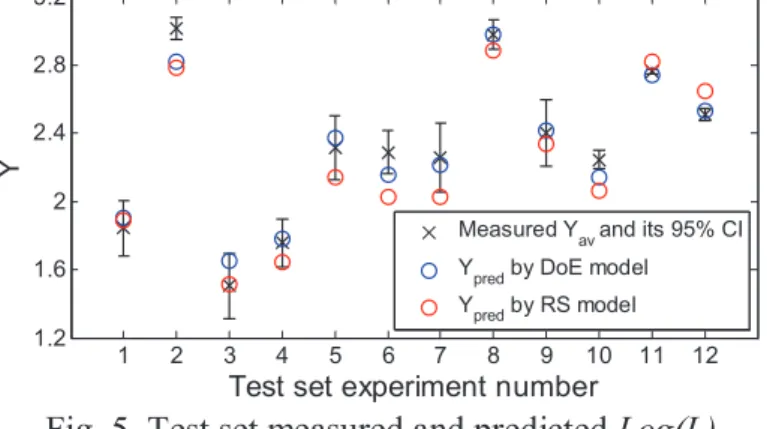
These models are then applied on the test set points (green points on Fig. 3). Fig. 5 shows, for these points, the predicted lifespan logarithms with respect to the corresponding measured Yav and their 95% CI. Table III summarizes model prediction
performance on the test set.
1 2 3 4 5 6 7 8 9 10 11 12 1.2 1.6 2 2.4 2.8 3.2
Test set experiment number
Y
Measured Yav and its 95% CI
Ypred by DoE model
Ypred by RS model
Fig. 5. Test set measured and predicted Log(L) TABLEIII
TEST SET PREDICTION PERFORMANCE OF DOEMODEL
Model Max (REY) Mean (REY) Max (REL) Mean (REL) DoE 9.7% 3.1% 35.0% 14.0% RS 11.5% 5.7% 45.1% 27.2%
7 Therefore, DoE model shows good prediction performance on the test set with an average error of 3% for predicted Y and of 14% for predicted L. Note that this error increase is due to the logarithmic back transformation applied on Y. However, the RS model presents higher errors on the test set with respect to DoE model. Therefore, the addition of 3 levels, 3 quadratic terms and 10 experimental points to the training set of DoE model over-fits the data and thus does not improve its prediction quality. Indeed, the oversizing of the model surely leads to an extremely accurate modelling of the training data. However, the counterpart is a decrease of the model flexibility and thus of its capacity to adapt to different experiment scenarios as those comprised in the test set [15].
From this test campaign, we can deduce that a first order parametric model estimated with only the 8 experiments of a 2-level FFD is sufficient for a good prediction of lifespan in the same experimental domain. Second order models with additional factor levels, quadratic terms and training set points can over-fit the data and lead to higher errors when applied on the test set.
3.2 Non-parametric models: regression trees
3.2.1 Principle
Previous models assume a multi-linear relationship between Log(L) and the three main factors, their quadratic forms and their interactions, allowing to quantify their respective effects. However, the interactions are introduced as independent explanatory variables through the product of the corresponding factors. This choice has no physical justification. Therefore, the interpretation of the resulting coefficients is not straightforward. Thus, it may be of interest to define another lifespan-stress relationship using the RS training set that could be more easily interpreted and could better fit the data than a second order model. Non-parametric Regression Trees (RT) present a first alternative approach to linear regression models and are especially appropriate when interactions exist between factors. To date, RT have never been applied in insulation aging studies. Classification and regression trees were introduced by Breiman in 1984 [16]. They allow to explain the relationship between a single response variable (output) and a set of predictor variables (inputs). The principle of RT is to recursively split the training data set into smaller and more homogeneous groups by selecting, at each node, the best separating variable and its best splitting value according to the model prediction performance. At each node, the splitting explanatory variable and its corresponding threshold value are selected so that the homogeneity of the two resulting groups is maximized. At the end, each leaf is characterized by the mean value of the response in the corresponding final group [16]. For a new observation, the response can be easily predicted by following the appropriate path throughout the tree. The order of appearance of the variables in the tree allows to compare their relative importance.
3.2.2 Regression Trees applied to Lifespan Modeling
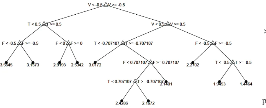
RT will be constructed using the RS training sets (18 blue and red experimental points of the CCD in Fig. 4) with factor levels XV, XF and XT as inputs and Log(L) as an output.
For a better readability, factors will be represented in the tree by V, F and T instead of XV,
XF and XT. RT performance will be evaluated on test sets (green points of Fig. 4). The RT
8 three voltage zones:
- Low Voltage (LV) where XV < -0.5 (V < 1.43 kV),
- High Voltage (HV) where XV > 0.5 (V > 2.10 kV),
- Medium Voltage (MV) where -0.5 < XV < 0.5.
As for parametric RS model, the voltage appears with RT as the most important variable since it first splits the data. The temperature is the next splitting variable in both LV and MV zones and finally comes the frequency. This order is coherent with factor effects estimated by RS model in Fig. 4b. However, frequency and temperature order of influence is inverted in HV zone. This fact reveals that the lifespan model is different in this voltage zone and that two different models exist depending on the voltage range: one corresponding to HV and the other to LV and MV zones that can be combined in one zone called MV&LV.
When used to predict the test set lifespan logarithms (Y) of this campaign (green points of Fig. 3), the RT displayed on Fig. 6a is less accurate than RS parametric model, with relative errors (ERY) up to 33%. Intrinsically, RT are piecewise constant models and thus
have lower prediction accuracy than parametric continuous models.
To illustrate this, Fig. 6b compares the measured Yav of the test set points, their values
predicted by the RT of Fig. 6a and by a linear model computed from the same training set and including only the three main factor terms (XV, XF and XT). It is clear from Fig. 6b
that the linear model better fits the test set points than the RT.
Fig. 6a. Regression tree constructed from the RS training set
1.2 1.6 2 2.4 2.8 3.2 1.2 1.6 2 2.4 2.8 3.2 Measured Yav Y p re d y=x Regression tree Linear model Fig. 6b. Prediction performance of the regression
tree and of a linear model including only the main factor
terms In conclusion, we can confirm that RT have lower prediction accuracy than parametric models since they are piecewise constant. However, RT allow to identify different ranges of the main factor corresponding to different models.
4.
Proposed approach: the hybrid models
4.1 Motivation
In light of the above, we can see that each presented model has its advantages and drawbacks. Parametric DoE and RS models allow quantifying the effects of each factor, of their quadratic terms and of their interactions on the lifespan with good prediction performance on the test set points belonging to the same experimental domain as the training set points. However, the second order models appear to over-fit the data although
9 estimated from an optimized training set. On the other hand, interpretation of the interaction effects through the product terms is not obvious.
With RT, a simple and graphical life-stress relationship is obtained. Relative importance of the main factors can be deduced from the hierarchical structure of the RT. This structure also allows to identify ranges of the main factor where more specific and thus more accurate models can be derived. However, RT are piecewise constant and have lower prediction performance on the test set than parametric models.
Therefore, we suggest in this section to combine these two approaches in a piecewise linear model in order to benefit from the advantages of the two methods and to overcome their drawbacks. The proposed model is thus called Hybrid Model (HM) and is presented as an original method based on RT for the lifespan modeling of insulation materials.
4.2 Principle
The principle of HM is related to the so-called model trees [17]. The basic idea is to derive a multilinear model for each leaf of the tree. Many sophisticated algorithms exist to build model trees. However, they are complex and the gain in performance is conditional upon the data size. In our case, where few experimental points are available, we propose a very simple implementation called hybrid model. first to identify the most important factor and its splitting values through the RT. Then, by the means of dummy variables, one coefficient for each of the two other factors is defined in each range of the main factor. This model structure allows to:
x Refine the parametric model by examining the life-stress relationship in each identified range
x Explicit interactions with the main factor by examining the effect of the main factor range on the coefficients of the other two factors, (interaction between the least important two factors have a very low effect according to parametric models),
x Improve the prediction quality of regression trees.
As RT, HM will be computed from the RS training set (blue and red points in Fig. 3) using the factor levels XV, XF and XT as predictors and Log(L) as a response where L is in
(s). Then the model prediction performance will be evaluated on the corresponding test set (green points of Fig. 43).
4.3 Hybrid models applied to Lifespan Modeling
Voltage was identified as the most important stress factor dividing RS training set into two ranges: HV and MV&LV at XV = 0.5. The HM can thus be written as (5):
Log(L)HM = M + EVXV + EF/HVGHV.XF + EF/MV&LVGMV&LV.XF + ET/HVGHV.XT +
ET/MV&LVGMV&LV.XT
(5) where GHV (respectively GMV&LV) is a dummy variable equal to 1 when XV belongs to HV
(respectively MV&LV) zone and 0 elsewhere. Equation (5) has the general form of a multi-linear regression model between the response Log(L) and the predictor variables XV, GHV.XF, GMV&LV.XF, GHV.XT and GMV&LV.XT. Model coefficients can thus be estimated by
OLS method. The coefficients of HM (5) estimated from the 18 points of RS training set (blue and red points of fig. 3) are represented in the diagram of Fig. 7.
10 -0.6 -0.4 -0.2 0 EV EF / H V EF / M V&LV ET / H V ET / M V&LV
Fig. 7 Hybrid Model coefficients
This model confirms once again that voltage is the most important factor for the studied material. It also confirms the existence of interactions between the voltage and the frequency (respectively the temperature) since two different coefficients exist for the frequency (respectively the temperature) depending on the voltage zone. In addition, the relative effects of frequency and temperature in each zone are coherent with their order in the RT of Fig. 6a: the frequency effect is lower than the temperature effect in MV&LV, but higher in HV.
HM (5) prediction performance on the test set (green points of Fig. 3) is summarized in Fig. 8 and Table IV. Obviously, HM model improves the prediction quality of both RT and RS models regarding the test set. Therefore, with the 18 points of an organized CCD as a training set, a piecewise first order model (HM) is more appropriate for data fitting than a second order model with interaction terms (RS).
1 2 3 4 5 6 7 8 9 10 11 12 1 1.5 2 2.5 3 3.5
Test set experiment number
Y
Measured Yav and its 95% CI Ypred by Hybrid Model
Fig. 8 Test set measured and predicted Log(L) TABLEIV
TEST SET PREDICTION PERFORMANCE OF HM
Max (REY) Mean (REY) Max (REL) Mean (REL) 8.7% 3.8% 35.6% 16.8%
From the test campaign, it was confirmed that a HM shows better prediction quality than RS parametric model, both being estimated from the same organized training set. In addition, experimental matrices of HM (5) and (6) are orthogonal since no quadratic terms are included. This property remains satisfied for all CCD, regardless to N0 and T,
and 3-level FFD3 as training sets for HM having the same form as (5) and (6). This property is an additional advantage for HM over RS models. It offers more flexibility for
11 the choice of the organized design of the training set. In both test campaigns, HM prediction performance is very close to that of DoE models computed from 2-level FFDs. However, HM involves a smaller number of variables than DoE model (6 instead of 8). All these variables are important and more easily interpretable than those of DoE model. Therefore, with k factors and only two levels per factor that can be tested, the best lifespan model configuration in terms of accuracy and experimental cost is a first order model with interaction terms computed from the 2k experiments of the 2-level FFD. If more levels per factor can be tested so that a CCD or a 3-level FFD can be established, the best lifespan model is a HM configured after identifying the different regions of the main stress factor with a RT constructed on the same training set.
Conclusion and Future Work
In conclusion, this paper proposed an original approach for the lifespan modeling of insulation materials under PD regime. This method was validated on an insulation material in an experimental domain corresponding to accelerated aging conditions. The presented models relate the lifespan logarithm to three main aging factors through three different forms: parametric, non-parametric and hybrid models. These models allow to evaluate the effects of the three factors and of their interactions. While parametric forms are commonly used in modeling tasks, non-parametric regression trees and hybrid models provide original life-stress relationships that have never been investigated in insulation aging studies before. These different models were compared and the optimal use of each was defined accordingly. In future work, the presented methodology will be applied to the lifespan modeling of other thermal class insulating materials and other critical parts of electrical machines. On the other hand, more stress factors will be considered in the insulation lifespan models such as pressure, humidity or mechanical vibrations. Finally, as prognostic is the final goal of this lifespan modelling, model prediction of long life aging during almost normal conditions will be investigated. For this objective, materials will be tested in domains below the PD regime in order to test the validity of the presented models at lower stress levels that are closer to normal conditions.
Acknowledgment
This work is has been supported by the Transversalité program for Toulouse’s Idex. References
[1] L. Fang, I. Cotton, Z.J. Wang and R. Freer, "Insulation Performance Evaluation of High Temperature Wire Candidates for Aerospace Electrical Machine Winding," in Proc. 2013 IEEE Electrical Insulation Conf., pp. 253-256.
[2] I. Christou, A. Nelms, I. Cotton and M. Husband, "Choice of optimal voltage for more electric aircraft wiring systems," IET Electr. Syst. Transp., vol. 1, no. 1, pp. 24-30, 2011.
[3] I. Christou, I. Cotton, "Methods for partial discharge testing of aerospace cables," in Proc. Conference Record of the 2010 IEEE International Symposium on Electrical Insulation (ISEI), pp. 1-5.
[4] D. F. Ortega, F. Castelli-Dezza, "On line partial discharges test on rotating machines supplied by IFDs," 2010 XIX IEEE International Conference on Electrical Machines (ICEM), pp. 1-4.
12 [5] Y. Jinkyu, B. L. Sang, Y. Jiyoon, L. Sanghoon, O. Yongmin and C. Changho, "A Stator Winding Insulation Condition Monitoring Technique for Inverter-Fed Machines," IEEE Transactions on Power Electronics, vol. 22, no. 5, pp. 2026-2033, 2007.
[6] P. J. Tavner, "Review of condition monitoring of rotating electrical machines," IET Electr. Power Appl., vol. 2, no. 4, pp. 215- 245, 2008.
[7] A. C. Gjerde, "Multifactor ageing models - origin and similarities," IEEE Electr. Insul. Mag., vol. 13, no 1, p. 6-13, 1997.
[8] STONE, G. C. The statistics of aging models and practical reality. Electrical Insulation, IEEE Transactions on, 1993, vol. 28, no 5, p. 716-728.
[9] L. Escobar and W. Meeker, "A review of accelerated test models," Stat. Sci., vol. 21, no. 4, pp. 552-577, 2006.
[10] F. Salameh, A. Picot, M. Chabert, and P. Maussion. (2015, Nov.). Regression methods for improved lifespan modeling of low voltage machine insulation. Math. Comput. Simul. Available: http://dx.doi.org/10.1016/j.matcom.2015.11.001
[11] R. A. Fisher, The Design of Experiments, Edinburgh, U.K.: Oliver and Boyd, 1935.
[12] R. H. Myers and D.C. Montgomery, Response Surface Methodology, New York: John Wiley and Sons, 2002.
[13] A. I. Khuri and J. A. Cornell, Response surfaces: designs and analyses. CRC press, 1996.
[14] American National Standards Institute, ANSI/NEMA MW 1000-2003, Revision 3, 2007.
[15] N. R. Draper and H. Smith. Applied regression analysis, 3rd ed., New York: Wiley, 1998.
[16] L. Breiman, J. H. Friedman, R. A. Olshen, and C. G. Stone. Classification and Regression Trees, California: Wadsworth, 1984.
[17] D. Malerba, F. Esposito. M. Ceci, A. Appice, "Top-down induction of model trees with regression and splitting nodes," IEEE Trans. on Pattern Analysis and Machine Intelligence, vol. 26, no. 5, May 2004.