The 2ndJoint International Conference on Multibody System Dynamics May 29–June 1, 2012, Stuttgart, Germany
Advanced Engine Dynamics Using MBS and a
Mixed Nonlinear FEM and Super Element Approach
Yannick Louvigny, Pierre DuysinxLTAS Automotive Engineering University of Liège
B52 Chemin des Chevreuils 1, B-4000 Liège, Belgium [email protected]
ABSTRACT
Dynamic simulations of a twin-cylinder boxer engine are carried out with rigid and flexible multibody models. Pistons and connecting rods are considered as rigid bodies while the crankshaft is modeled as a flexible part and meshed with brick elements. With this model, calculation of crankshaft stresses and displacements is possible. For constant speed studies, flexible simulations are carried out on one or two engine cycles but simulations with a variable rotation speed has to be performed on a larger number of engine revolutions. Due to the complex shape of the crankshaft, the simulation times become important and it is difficult to keep on working with the complete crankshaft model. Thus several simplified models, including super element models, are developed. In this paper, a particular method, using also the super element technique, is proposed. A large part of the crankshaft is substructured and modeled with super elements. While a critical area, identified by a simulation performed with a coarse crankshaft mesh, is not modified and modeled by nonlinear finite element. Several methods of linking the super elements and the finite element mesh are experimented. Once the best connection method determined, results and computation time of the simulation using this model will be compared to those obtained with the complete crankshaft model and the other simplified models.
1 INTRODUCTION
Dynamic simulations of a twin-cylinder boxer engine are carried out, in SAMCEF FIELD MECANO soft-ware, with rigid and flexible multibody models using the finite element approach (described by Géradin and Cardona in [1]). The CAD drawing of the two pistons, two connecting rods and crankshaft are imported in the SAMCEF FIELD environment and the parts are linked together using appropriate kinematic joints. The gas pressure in the cylinder is modeled by resultant forces applied on the pistons upper face. Pistons and connecting rods are considered as rigid bodies while the crankshaft is modeled as a flexible part and meshed with brick elements. With this model, calculation of crankshaft stresses and displacements is possible. For constant speed studies, flexible simulations are carried out on one or two engine cycles but simula-tions with a variable rotation speed has to be performed on a larger number of engine revolusimula-tions. Due to the complex shape of the crankshaft, the simulation times become important and it is difficult to keep on working with the complete crankshaft model. So, simplified crankshaft models have been developed:
• A tridimensional model, described in [2], with simplified geometry (no fillet radius, no lubrication
hole. . . )
• A beam model, also described in [2]. • A super element model, presented in [3].
• A mixed model using FEM and super element technique.
2 OBJECTIVES
In this paper, a mixed method, using super element technique and classical finite element approach, is pro-posed, this approach has been described by Heege et al. in [6]. A large part of the crankshaft is substructured
and modeled by one or more super elements. While a specific area is not modified and modeled by nonlinear finite element. This specific part of the crankshaft has been identified as a critical part in a previous flexible multibody simulation, performed with a coarse crankshaft mesh, because it presented the highest stresses values. It is the crankpin located on the distribution side.
Several methods of linking the super elements and the finite element mesh have been experimented. The crankshaft stresses calculated with these different linking methods have been compared with the ones calcu-lated with a fully meshed model of the crankshaft. Once the best connection method determined, results and computation time of the simulation using this method will be compared to those obtained with the complete crankshaft model and the other simplified models.
3 MODELING
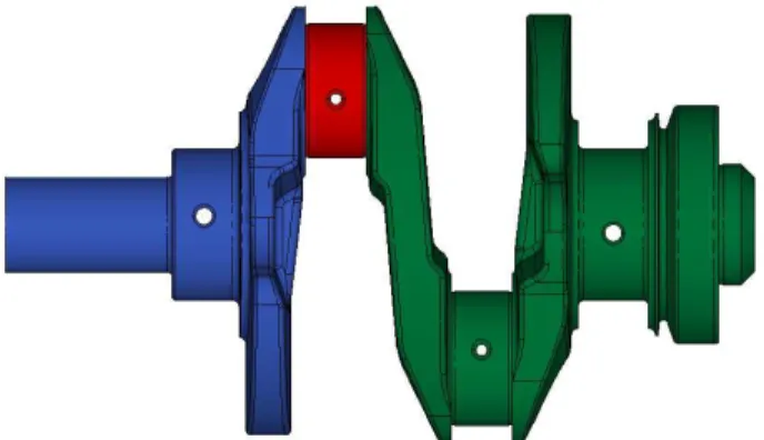
The crankshaft is separated in three parts:
• The critical crankpin (colored in red in figure1),
• The crankshaft section that is on the left of the studied crankpin (colored in blue in figure1), • The crankshaft section that is on the right of the studied crankpin (colored in green in figure1).
Figure 1. The three parts of the crankshaft model.
The crankpin is considered as a flexible body and is studied using finite element technique. It is meshed (illustrated in figure2) with 11300 tetrahedral elements (the average edge size of a tetrahedron is 3 mm). Each one of the two adjacent parts of the crankshaft is modeled with a super element.
The super element approach is a substructure technique used to reduce the size of a problem. It consists in subdividing a structure in components called super elements, which are analyzed and condensed separately, while preserving the junction dofs between substructures. The super elements are represented by their modes including vibration normal modes, rigid body modes, etc [4]. It required three steps; the first one is the condensation step when some dofs are eliminated to reduce the size of the stiffness and mass matrices. Indeed, the dynamic behavior of one subsystem can be fully described by its boundary dofs and its natural frequencies [5]. Once the super element is created, it must be assembled in the global system that can then be solved, it is the second step. Finally, some specific results of the super element, for instance the strains and stresses, can be recovered by a dynamic analysis of the super element. In a previous work [3], it has been demonstrated that the super element model of the crankshaft allows important reductions of CPU time, which was its main purpose. But it offers other advantages with respect to the initial complex model:
• If the goal is not to determine the results for the complete simulation, then it is possible to recover
them for a limited number of time step to reduce computing time.
• It permits also a direct decoupling of the displacements coming from the deformation and the ones
Figure 2. Crankshaft model using FEM and super elements.
The three crnakshaft pieces are linked together using “glue” assembly constraints. The glue assembly of SAMCEF FIELD is used to connect nodes on two different supports. The connected nodes on the second support will follow exactly the same movement as those on the first support.
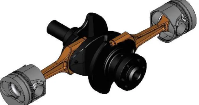
Then, the crankshaft mixed model is imported in the engine model (illustrated in figure3). The latter includes two pistons and two connecting rods considered as rigid bodies. The crankshaft is constrained by ground hinge joints connected to its main journals. A prescribed rotation speed constraint is applied on the crankshaft face where the flywheel is normally connected. The rotation speed is chosen equal to 4000 rpm which is the speed corresponding to the engine maximal power and it is close to the engine maximum rotation speed where the inertia effect will be maximum. The connecting rods are linked to the pistons and to the crankpins by hinge joints. Some translation and rotations degrees of freedoms of the pistons are locked to simulate the contact between the piston and the cylinder wall. A variable resultant force, depicting the gas pressure effect, is applied on each piston top face.
Figure 3. Engine including the mixed model of crankshaft.
Then, we simulate the engine dynamic during 0.06 seconds which corresponds to two complete engine cycles (four revolutions) at 4000 rpm. The time integration scheme used for this simulation is an implicit Chung-Hulbert algorithm where the simulation results are saved every 41.667 µs i.e. every degree of crankshaft rotation.
4 RESULTS
As one of the main assets of the finite element approach is the ability to simulate flexible bodies and to determine their mechanical stresses, we will focus, in this section, on the crankshaft stress values. In order to compare the results obtained here with the results obtained with other models previously established
(fully meshed crankshaft model and full super element model), three criteria are studied in this paper:
• The computing time of the simulation,
• The maximum stress (its value, its location and the instant when it occurs) and the stress distribution
in the crankpin at that moment,
• The stress value of a crankpin particular node during the simulation.
The computing time of this simulation (16000 DOFs and 1440 time steps) is 7,5 hours on a standard com-puter (quad-core 2.8 GHz - 4 Gb RAM).
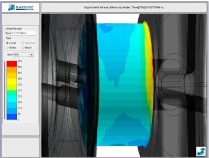
The maximum stress values is 541 MPa (Von Mises criterion, mean value by node) and occurs at 0.015775 second that corresponds to a crankshaft angular position of 18.6 degrees after the top dead center when the combustion begins in the associated cylinder. This angle of 18.6 degrees corresponds to a crankshaft position where the force coming from the connecting rod and acting on the crankpin is between its maximum radial value and maximum tangential value [2]. The highest stresses are located in the fillet between the crankpin and the outside crankshaft arm and the maximum value is reached in the part of the fillet facing the counterweight. Outside fillets, the stress intensity is much lower (<200 MPa).
Figure 4. Maximum stress calculated with the crankshaft mixed model.
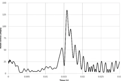
After studying the stress distribution at a given time, we focus on the stress evolution during the engine cycle. For this purpose, the stress versus time curve is plotted for a specific node. This node has been chosen in the middle of the contact surface of the crankpin, just in front of the piston when the crankshaft angle is null (see figure5).
The curve in figure6illustrates the stresses variation of this specific crankpin area during one complete engine cycle. One notices that the stress reachs a maximum at time 0.01578 second, which is also the instant when the absolute maximum crankpin stresses are observed. But at this location, the intensity is much lower and the maximum value is 135 Mpa. Excluding the stress peak due to the fuel combustion, during the rest of the engine cycle, the stress values do not even exceed 60 Mpa and oscillate around 25 Mpa.
5 COMPARISON
We will now perform the same simulation using a crankshaft entirely modeled with finite elements which will be our reference model and a model of crankshaft obtained with super element technique.
Figure 5. Selection of the monitored node.
Figure 6. Stress values at the selected node for the crankshaft mixed model.
The reference crankshaft is meshed with the same type and same size of finite elements as the crankpin of the first model. The computing time of the simulation with this model (169000 DOFs and 1440 time steps) is 50 hours on the same computer (quad-core 2.8 GHz - 4 Gb RAM). One notices that the computing time is nearly seven times longer than the time of the simulation using the mixed model. Furthermore, the size of the problem will lead to memory problems to visualize the results.
The super element crankshaft is built on the basis of the previous crankshaft mesh. With this model, the computing time of the simulation (64000 DOFs and 1440 time steps) is 10 hours on the same computer (quad-core 2.8 GHz - 4 Gb RAM), which is approximately 30% longer than the simulation using the mixed model. Moreover, it needs the recovery step which is not necessary with the mixed model if one is interested only in the crankpin stresses. Nevertheless, this recovery step gives access to the crankshaft deformations, which is not possible with the two other models.
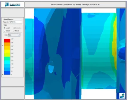
In the reference simulation (using the finite elements crankshaft), the maximum stress values, shown in figure7, is 445 MPa and occurs at 0.01578 second which corresponds to a crankshaft angular position of 18.7 degrees after the top dead center. One can notice that the value of the maximum stress is lower than the one calculated with the mixed model, 445 MPa instead of 541 MPa what makes a difference of 21%. But, the moment and the position where this high stress occurs are identical. The stress distribution in the rest of the crankpin is quite consistent between the two models. This problem of maximum stress evaluation probably comes from the fact that the overstress occurs in the area where the finite elements and super elements are glued in the crankshaft mixed model.
Figure 7. Maximum stress calculated with the crankshaft full model.
figure8, is 447 MPa and occurs at 0.015795 second that corresponds to a crankshaft angular position of 19 degrees after the top dead center. The results given by this super element model coincides perfectly with those of the reference model.
Figure 8. Maximum stress calculated with the crankshaft super element model.
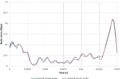
We will now compare the stress evolution in the chosen node for reference crankshaft and the crankshaft mixed model. The stress versus time curves of the two models are plotted in figure9. One can notice that the stress calculation, for a point in the middle of the crankpin surface, is consistent between the reference and the mixed model.
Figure 9. Stress values at the selected node for several crankshaft models.
6 CONCLUSIONS
A particular method, using a mixed of finite elements and super elements in the modeling of the same object, has been proposed. Crankpin stresses and computation time of the simulation using this model have been compared to those obtained with the complete crankshaft model and a super element model. The comparison of stress distributions has shown that the studied model worked well except for the overstresses evaluation at the limit of the critical area. The latter problem can be avoided by enlarging a bit the area modeled in finite elements. In terms of computation time, this model was superior to the two other ones, very far from the complete finite elements model and a bit faster compared to the model using only super elements but this latter offers other advantages such as the visualization of the deformation. In conclusion, this method offers several advantages over the other mentioned models and deserves some further attention.
REFERENCES
[1] Géradin, M.; Cardona, A.: Flexible Multibody Dynamics: a Finite Element Approach. John Wiley & Sons, 2001.
[2] Louvigny, Y.; Duysinx, P.: Advanced Engine Dynamics using MBS: Application to twin-Cylinder Boxer Engines. In Proceedings of the 1st Joint International Conference on Multibody System Dynamics, Lappeenranta, May 2010.
[3] Louvigny, Y.; Duysinx, P.: Advanced Engine Dynamics using MBS and Super Element Approach: Application to Twin-Cylinder Boxer Engines. In Proceedings of the ECCOMAS Thematic Confer-ence in Multibody Dynamics, Brussels, July 2011.
[4] Masson, G.; Ait Brik, B.; Cogan, S.; Bouhaddi, N.: Component Mode Synthesis (CMS) Based on an Enriched Ritz Approach for Efficient Structural Optimization. Journal of Sound and Vibration, Vol. 296, pp. 845–860, 2006.
[5] Qu, Z.Q.: Model Order Reduction Techniques: with Applications in Finite Element Analysis. Springer, 2004.
[6] Heege, A.; Adolphs, G.; Lucas, P.; Sanchez, J.L.; Bonnet, P.; Diez, F.: Fatigue Damage Computation of a Composite Material Blade using a “Mixed non-linear FEM and Super Element Approach”. In Proceedings of The Europe’s Premier Wind Energy Event, Brussels, March 2011.