Cl´ement Berenfeld∗ and Marc Hoffmann†
October 18, 2019
Abstract
We investigate density estimation from a n-sample in the Euclidean space RD, when the data is supported by an unknown submanifold M of possibly unknown dimension d< D under a reach condition. We study nonparametric kernel methods for pointwise and integrated loss, with data-driven bandwidths that incorporate some learning of the geometry via a local dimension estimator. When f has H¨older smoothness β and M has regularity α in a sense close in spirit to (Aamari and Levrard, 2019), our estimator achieves the rate n−α∧β/(2α∧β+d) and does not depend on the ambient dimension D and is asymptotically minimax for α ≥ β. Following Lepski’s principle, a bandwidth selection rule is shown to achieve smoothness adaptation. We also investigate the case α≤ β: by estimating in some sense the underlying geometry of M, we establish in dimension d= 1 that the minimax rate is n−β/(2β+1) proving in particular that it does not depend on the regularity of M . Finally, a numerical implementation is conducted on some case studies in order to confirm the practical feasibility of our estimators.
Mathematics Subject Classification (2010): 62C20, 62G05, 62G07.
Keywords: Point clouds, manifold reconstruction, nonparametric estimation, adaptive density estimation, kernel methods, Lepski’s method.
1
Introduction
1.1 Motivation
Suppose we observe a n-drawn (X1, . . . , Xn) distributed on an Euclidean space RD according to some density function f . We wish to recover f at some point arbitrary point x∈ RD nonparamet-rically. If the smoothness of f at x measured in a strong sense is of order β – for instance by a H¨older condition or with a prescribed number of derivatives – then the optimal (minimax) rate for recovering f(x) is of order n−β/(2β+D) and is achieved by kernel or projection methods, see e.g. the classical textbooksDevroye and Gy¨orfi(1985);Silverman(1986) or (Tsybakov,2008, Sec. 1.2-1.3). Extension to data-driven bandwidths (Bowman,1984;Chiu,1991) offers the possibly to adapt to unknown smoothness, see (Goldenshluger and Lepski,2008, 2014;Goldenshluger et al., 2011) for a modern mathematical formulation. In many situations however, the dimension D of the ambi-ent space is large, hitherto disqualifying such methods for pratical applications. Opposite to the curse of dimensionality, a broad guiding principle in practice is that the observations(X1, . . . , Xn) actually live on smaller dimensional structures and that the effective dimension of the problem is
∗Cl´ement Berenfeld, Universit´e Paris-Dauphine & PSL, CNRS, CEREMADE, 75016 Paris, France. email:
beren-feld@ceremade.dauphine.fr
†
Marc Hoffmann, Universit´e Paris-Dauphine & PSL, CNRS, CEREMADE, 75016 Paris, France. email: hoff-mann@ceremade.dauphine.fr
smaller if one can take advantage of the geometry of the data (Fefferman et al.,2016). This classi-cal paradigm probably goes back to a conjecture of (Stone,1982) that paved the way to the study of the celebrated single-index model in nonparametric regression, where a structural assumption is put in the form f(x) = g(⟨ϑ, x⟩), where ⟨⋅, ⋅⟩ is the scalar product on RD, for some unknown univariate function g ∶ R→ R and direction ϑ ∈ RD. Under appropriate assumptions, the minimax rate of convergence for recovering f(x) with smoothness β drops to n−β/(2β+1)and does not depend on the ambient dimension D, see e.g. (Ga¨ıffas and Lecu´e, 2007; Lepski and Serdyukova, 2014) and the references therein. Also, in the search for significant variables, one postulates that f only depends on d< D coordinates, leading to the structural assumption f(x1, . . . , xD) = F(xi1, . . . xid)
for some unknown function F ∶ Rd→ R and {i
1, . . . , id} ⊂ {1, . . . , D}. In an analogous setting, the minimax rate of convergence becomes n−β/(2β+d) and this is also of a smaller order of magnitude than n−β/(2β+D), see (Hoffmann and Lepski,2002) in the white noise model.
The next logical step is to assume that the data (X1, . . . , Xn) live on a d-dimensional sub-manifold M of the ambient space RD. When the manifold is known prior to the experiment, nonparametric density estimation dates back to (Devroye and Gy¨orfi, 1985) when M is the circle, and on a homogeneous Riemannian manifold by (Hendriks,1990), see alsoPelletier(2005). Several results are known for specific geometric structures like the sphere or the torus involved in many ap-plied situations: inverse problems for cosmological data (Kerkyacharian et al.,2011;Kim and Koo,
2002;Kim et al.,2009), in geology (Hall et al.,1987) or flow calculation in fluid mechanics ( Euge-ciouglu and Srinivasan,2000). For genuine compact homogeneous Riemannian manifolds, a general setting for smoothness adaptive density estimation and inference has recently been considered by
Kerkyacharian et al. (2012), or even in more abstract metric spaces in Cleanthous et al. (2018). A common strategy adapts conventional nonparametric tools like projection or kernel methods to the underlying geometry, via the spectral analysis of the Beltrami-Laplace operator on M . Under appropriate assumptions, this leads to exact or approximate eigenbases (spherical harmonics for the sphere, needlets and so on) or properly modified kernel methods, according to the Riemannian metric on M .
If the submanifold M itself is unknown, getting closer in spirit to a dimension reduction ap-proach, the situation becomes drastically different: M hence its geometry is unknown, and consid-ered as a nuisance parameter. In order to recover the density f , one has to understand the minimal geometry of M that must be learned from the data and how this geometry affects the optimal reconstruction of f . This is the topic of the paper.
1.2 Main results
We construct a class of compact smooth submanifolds of dimension d of the Euclidean space RD, without boundaries, that constitute generic models for the unknown support of the target density f that we wish to reconstruct under a reach condition. The reach is a somehow unavoidable notion in manifold reconstruction that goes back toFederer(1959): it is a geometric invariant that quantifies both local curvature conditions and how tightly the submanifold folds on itself. It is related to the scale at which the sampling rate n can effectively recover the geometry of the submanifold, see Section 2.2 below. We consider regular manifolds M with reach bounded below that satisfy the following property: M admits a local parametrization at every point x∈ M by its tangent space TxM, and this parametrization is regular enough. A natural candidate is given by the exponential map expx ∶TxM → M ⊂ RD. More specifically, for some regularity parameter α≥ 1, we require a certain uniform bound for the α-fold differential of the exponential map to hold, quantifying in some
sense the regularity of the parametrization in a minimax spirit. Our approach is close but slightly more restrictive than Aamari and Levrard(2019, Def. 1) that consider arbitrary parametrizations among those close to the inverse of the projection onto tangent spaces. Given a density function f ∶ M → [0, ∞) with respect to the volume measure on M, we have a natural extension of smooth-ness spaces on M by requiring that f○ expx∶ TxM → R is a smooth map in any reasonable sense, see for instanceTriebel(1987) for the characterisation of function spaces on a Riemannian manifold. Our main result is that in order to reconstruct f(x) efficiently at a point x ∈ RD when f lives on an unknown smooth submanifold, it is sufficient to consider estimators of the form
̂ fh(x) = 1 nhd(x)̂ n ∑ i=1 K(x1 h , . . . , xD h ) , x = (x1, . . . , xD) ∈ R D, (1) where K ∶ RD → R is a kernel verifying certain assumptions and ̂d(x) = ̂d(x, X
1, . . . , Xn) is an estimator of the local dimension of the support of f in the vicinity of x based on a scaling estima-tor as introduced in Farahmand et al. (2007). We prove in Theorem 1 that following a classical bias-variance trade-off for the bandwidth h, the rate n−α∧β/(2α∧β+d) is achievable for pointwise and global loss functions (in Lp(M)-norm for p ≥ 1) when the dimension of M is d, irrespectively of the ambient dimension D. In particular, it is noteworthy that in terms of manifold learning, only the dimension of M needs to be estimated. When α≥ β, we also have a lower bound (Theorem2) showing that our result is minimax. Moreover, by implementing Lepski’s principle (Lepskii,1992), we are able to construct a data driven bandwidth ̂h= ̂h(x, X1. . . , Xn) that achieves in Theorem 3 the rate n−α∧β/(2α∧β+d) up to a logarithmic term — unavoidable in the case of pointwise loss due to the Lepski-Low phenomenon (Lepski˘ı,1990;Low, 1992). When the dimension d is known, the estimator (1) has already been investigated in squared-error norm in Ozakin and Gray (2009) for a fixed manifold M and smoothness β= 2.
A remaining question at this stage is to understand how the regularity of M can affect the minimax rates of convergence for smooth functions, i.e. when α≤ β. We restrict our attention to the one-dimensional case d= 1. When M is known, Pelletier (2005) studied an estimator of the form 1 nhd n ∑ i=1 1 ϑx(Xi) K(dM(x, Xi) h ) (2)
where K∶ R → R is a radial kernel, dM is the intrinsic Riemannian distance on M and the correction term ϑx(Xi) is the volume density function on M (Besse,1978, p. 154) that accounts for the value of the density of the volume measure at Xi in normal coordinates around x, taking into account how the submanifold curves around Xi. By establishing in Lemma 3 that ϑx is constant (and identically equal to one) when d= 1, we have another estimator by simply learning the geometry of M via its intrinsic distance dM in (2). This can be done by efficiently estimating dM thanks to the Isomap method as coined byTenenbaum et al.(2000). We construct an estimator that achieves in Theorem5the rate n−β/(2β+1), therefore establishing that in dimension d= 1 at least, the regularity of the manifold M does not affect the minimax rate for estimating f even when M is unknown. However, the volume density function ϑx is not constant as soon as d ≥ 2 and obtaining a global picture in higher dimensions remains open.
1.3 Organisation of the paper
In Section 2, we provide with all the necessary material and notation from classical geometry for the unfamiliar reader, as well as the essential notions we need from manifold learning. We elaborate
in particular on the reach of a subset of the Euclidean space in Section 2.2 and on our statistical model for density estimation on an unknown manifold in Section2.3. Section3 describes in details our estimator and its minimax properties in Theorem 1 and Theorem 2 as well as its adaptation properties with respect to an unknown smoothness (Theorem 3). For clarity, we first consider the case when the dimension d and regularity α of the submanifold M and the smoothness β of the density are known (Section 3.3). We next treat adaptation with respect to α and β (Section3.4). Finally, we consider adaptation with respect to β and d in Section3.5and construct an estimator in Theorem4 that adapts to the smoothness of f and the dimension of M simultaneously. Section 4
focuses on the case on one-dimensional submanifolds, where we prove that the regularity of the underlying geometry does not affect the minimax rates of convergence for estimating f pointwise (Theorem5). Finally, numerical examples are developed in Section5: we elaborate on examples of non-isometric embeddings of the circle and the torus in dimension 1 and 2 and explore in particular rates of convergence on Monte-Carlo simulations, illustrating how effective Lepski’s method can be in that context. The proof are delayed until Section6.
2
Manifold-supported probability distributions
2.1 Submanifolds of RD
We recall some basic notions of geometry of submanifolds of the Euclidean space RD for the unfamiliar reader. We borrow material from the classical textbooks Gallot et al. (2004) and Lee
(2006). We endow RD with its usual Euclidean product and norm, respectively denoted by ⟨⋅, ⋅⟩ and ∥ ⋅ ∥. We denote by BD(x, r) the open ball of RD of center x and radius r.
Smooth submanifolds and tangent spaces
A smooth submanifold M of RD is a connected subset of RD that verifies (Gallot et al., 2004, Prp 1.3 p.3) that for any point x∈ M, there exists an open neighbourhood of x in RD and a smooth map (called a parametrization) φ ∶ Ω→ RD defined in a neighbourhood Ω of 0 in Rdfor some d≥ 1 and such that φ(0) = x; dφ(0) is injective; and φ is a homeomorphism from Ω onto U ∩ M. The integer d, called the dimension of M , is the same for all local parametrizations of M . A vector v∈ RD is said to be tangent to M at point x∈ M if there exists a smooth curve γ ∶ I → M defined in a neighbourhood of 0 in R and such that γ(0) = x and ˙γ(0) = v. The set of all tangent vectors at point x∈ M is called the tangent space and is denoted by TxM. It is a subspace of RD of dimension dand it verifies that for any local parametrization φ of M at x, we have TxM = dφ(0)[Rd] (Gallot
et al.,2004, Thm. 1.22 and 1.23 p.13). We denote by TxM⊥ the orthonormal complement of TxM in M , also called the normal space at point x.
Geodesics and the exponential map
A smooth curve γ ∶ I → M defined on an open set I of R is called a geodesic if at any time t ∈ I, the acceleration ¨γ(t) lies in the normal space Tγ(t)M⊥ (Gallot et al., 2004, Ex 2.80 b. p.81). In particular, the speed t↦ ∥ ˙γ(t)∥ of a geodesic is constant. For any x ∈ M and any v ∈ TxM, there exists a unique maximal geodesic γx,v defined in an open neighbourhood of 0 such that γx,v(0) = x and ˙γx,v(0) = v (Gallot et al.,2004, Cor 2.85 p.85). The set of vectors v ∈ TxM such that γx,v(1) is well defined is a neighbourhood of 0 in TxM. We define on this neighbourhood the map
called the exponential map. It is smooth and there always exists ǫ> 0 such that its restriction to the ball Bd(0, ǫ) in TxM defines a local parametrization of M at point x (Gallot et al., 2004, Cor 2.89 p.86). The supremum of all ǫ for which the latter holds true is called the injectivity radius at point x.
The uniqueness of γx,v readily yields that expx(tv) = γx,v(t), for any t ∈ R for which both expressions are well-defined, in particular in a neighbourhood of 0. Letting t go to 0 shows that dexpx(0) = IdTxM and that d
2exp
x(0)[v ⊗ v] = ¨γx,v(0) ∈ TxM⊥. The map d2expx(0) is denoted by IIx and is called the second fundamental form of M at x — seeGallot et al. (2004, Def 5.1 p. 246) for a more general definition. The quantity IIx(v ⊗ v) encapsulates the way the submanifold M curves around x in the direction v. For instance, if M is flat around x, then the geodesics originating from x are locally straight lines and thus IIx= 0.
Length of curves and the Riemannian distance
We say that a curve γ ∶ [a, b] → M with a < b is admissible if there exists a finite subdivision a = a0 < ⋅ ⋅ ⋅ ≤ ak−1 < ak = b of [a, b] such that on any segment [ai, ai+1], γ is smooth and its derivative does not vanish. For such a curve, we define its length as
L(γ) = ∫ b
a ∥ ˙γ(t)∥dt.
For any two points x, y ∈ M, we define the Riemannian distance dM(x, y) between x and y as the infimum of the length of all the admissible curves that join x to y. One can show that dM is well-defined on M × M (recall that we only consider connected submanifolds) and that it is indeed a distance. It endows M with a topology that coincides with the one induced by the ambient space, see Lee(2006, Lem 6.2 p.94) and Arias-Castro and Le Gouic(2019, Lem 3). An admissible curve γ that reaches the infimum in the definition of dM is called minimizing. We know that every minimizing curve is a geodesic of M , up to a reparametrization (Lee,2006, Thm 6.6 p.100). Conversely, if y is in expx(Bd(0, ǫ)) with ǫ smaller than the injectivity radius at x, then the geodesic joining x and y is minimising (Lee,2006, Prp 6.10). This means that for any v∈ TxM with∥v∥ < ǫ, we have dM(x, expx(v)) = ∥v∥.
When M is a closed subset of RD, the maximal geodesics γ
x,v are defined on the whole line R, and the exponential maps are defined on the whole tangent spaces. This is (one side of) the Hopf-Rinow theorem (Lee,2006, Thm 6.13 p.108).
The volume measure
We need a canonical way to define a uniform measure µM on M . This can easily be done locally around x∈ M by pushing forward the Lebesgue measure on TxM through expx∶BTxM(0, ǫ) → M
with ǫ smaller than the injectivity radius at x. In order to take into account the geometry of M around x, we add a correction term, called the volume density function (Besse,1978, p. 154). For a continuous function ψ ∶ M → R with support in expx(Bd(0, ǫ)), we define
µM(ψ) = ∫ Bd(0,ǫ)
ψ ○expx(v)√det gx ij(v)dv, with gx
ij(v) = ⟨d expx(v)[ei], d expx(v)[ej]⟩ and where (e1, . . . , ed) is an arbitrary orthonormal basis of TxM. The value of
√ det gx
ij(v) represents the volume of the parallelepiped in Texpx(v)M
gen-erated by the images of (e1, . . . , ed) via d expx(v). We can then define µM(ψ) for any continuous bounded ψ ∶ M → R by means of partition of unity (Gallot et al.,2004, Sec 1.H), see Gallot et al.
(2004, Sec 3.H.1 and Sec 3.H.2) for further details. The volume of M , denoted by vol M , is then simply µM(✶). It is finite if M is a compact submanifold of RD.
There is another natural candidate for a measure on M , namely the restriction of the d-dimensionnal Hausdorff measure Hd to M , see Federer (1969, Sec 2.10.2 p.171) for a definition. Luckily, we have µM(A) = Hd(A) for any Borel subset A ⊂ M (Evans and Gariepy, 1992, Ex D p.102).
2.2 The reach of a subset in an Euclidean space
One of the main concern when dealing with observations sampled from a geometrically structured probability measure is to determine the suitable scale at which one should look at the data. Indeed, given finite-sized point cloud in RD, there are infinitely many submanifolds that interpolate the point cloud, see Figure 1 for an illustration. A popular notion of regularity for a subset of the Euclidean space is the reach, introduced by Federer(1959).
Figure 1: An arbitrary points cloud (Left) for D = 2, and two smooth one-dimensional submanifolds passing through all its points (Middle, Right). A reach condition tends to discard the Right manifold as a likely candidate among all possible submanifolds the point cloud is sampled from.
Definition 1. Let K be a compact subset of RD. The reach τK of K is the supremum of all r≥ 0 such that the orthogonal projection prK on K is well-defined on the r-neighbourhood Kr of K, namely
τK = sup{r ≥ 0 ∣ ∀x ∈ RD, d(x, K) ≤ r ⇒ ∃!y ∈ K, d(x, K) = ∥x − y∥}.
When M is a compact submanifold of RD, the reach τM quantifies two geometric invariants: locally, it measures how curved the manifold is, and globally, it measures how close it is to inter-sect itself (the so-called bottleneck effect). See Figure 2 for an illustration of the phenomenon. A reach condition, meaning that the reach of the manifold under study is bounded below, is usually necessary in order to obtain minimax inference results in manifold learning. These include: ho-mology inference Balakrishnan et al.(2012);Niyogi et al. (2008), curvature (Aamari and Levrard,
2019) and reach estimation itself (Aamari et al.,2019) as well as manifold estimationAamari and Levrard(2019);Genovese et al.(2012). We follow this approach, and start with citing a few useful properties related to the reach.
Proposition 1. (Niyogi et al.,2008, Prp. 6.1) Let M be a compact smooth submanifold of RD. Then, for any x∈ M, we have ∥ IIx∥op≤ 1/τM.
Since IIxis the differential of order two of the mapping expx, Proposition1has several convenient implications. First, it gives a uniform lower bound for the injectivity radiuses of M . This is a corollary of Alexander and Bishop (2006, Thm 1.3), as explained in Aamari and Levrard (2019, Lem A.1).
Figure 2: For the first manifold M (Left), the value of the reach τM comes from its curvature. For the second one (Right), the reach is equal to τM because it is close to self intersecting (a bottleneck effect). The blue area represents the tubular neighbourhood over which the orthonormal projection on each manifold is well-defined.
Proposition 2. Let M be a compact smooth submanifold of RD. Then, for any x ∈ M, the exponential map expx∶ TxM→ M is a diffeomorphism from Bd(0, πτM) to expx(Bd(0, πτM)).
Proposition 1also yields nice bounds on how well the Euclidean distance on RD approximates the Riemannian distance dM on M× M.
Proposition 3. (Niyogi et al., 2008, Prp. 6.3) For any compact submanifold M of RD and any x, y∈ M such that ∥x − y∥ ≤ τM/2, we have
∥x − y∥ ≤ dM(x, y) ≤ τM⎛ ⎝1− √ 1−2∥x − y∥ τM ⎞ ⎠.
Proposition 3 allows in turn to compare the volume measure µM to the Lebesgue measure on its tangent spaces.
Lemma 1. For any d-dimensional compact smooth submanifold M of RD, for any x∈ M and any η≤ τM/2, we have, for all h ≤ η
(1 − η2/6τ2
M)dζdhd≤ µM(BD(x, h)) ≤ {(1 + (ξ(η/τM)η)2/τM2 )ξ(η/τM)}dζdhd where ξ(s) = (1 −√1− 2s)/s and ζd is the volume of the unit Euclidean ball in Rd.
Proof. This result already appears in (Aamari, 2017, Lem III.23) but we prove it here to make constants explicit. Let us denote by Leb the Lebesgue measure on TxM. Using (Aamari,2017, Prp III.22.v), we know that, as long as ξ(h/τM)h ≤ τM (which holds if h≤ τM/2),
(1 − h2/6τ2)dLeb(B d(0, h)) ≤ µM( expx(Bd(0, h))) ≤ µM( expx(Bd(0, ξ(h/τM)h))) ≤ (1 + (ξ(h/τM)h)2/τM2 ) d Leb(Bd(0, ξ(h/τM)h)).
Thanks to Proposition3, if h≤ τM/2, then expx(Bd(0, h)) ⊂ M∩BD(x, h) ⊂ expx(Bd(0, ξ(h/τM)h)). These inclusions combined with the last inequalities yield the result.
2.3 A statistical model for sampling on a unknown manifold
Our statistical model is characterised by two quantities: the regularity of its support and the regularity of the density defined on this support. The support belongs to a class of submanifolds
M, for which we need to fix some kind of canonical parametrization. This is what Aamari and Levrard (2019) propose by asking the support M to admit a local parametrization at all point x ∈ M by TxM, and that this parametrization is close to being the inverse of the projection over this tangent space. We consider here a somewhat stronger condition: among all the local parametrizations of a manifold by its tangent spaces, we impose a constraint on the exponential map up to its differentials of order k.
Definition 2. Let 1≤ d < D be integers and τ > 0 be a positive number. We let Cd(τ) define the set of submanifolds M of RD satisfying the following properties:
(i) (Dimension) M is a smooth submanifold of dimension d without boundaries; (ii) (Compactness) M is compact;
(iii) (Reach condition) We have τM ≥ τ.
For a real number α ≥ 1 and a positive real number L > 0, we define Cd,α(τ, L) of as the set of M ∈ Cd(τ) that fulfill the additional condition:
(iv) For any x∈ M the restriction of the exponential map expx to the ball BTxM(0, τ/2) is
(α+1)-H¨older with coefficient L. Namely, setting k= ⌈α⌉ and δ = α + 1 − k > 0, we have ∀v, w ∈ BTxM(0, τ/2), ∥d
k
expx(v) − dkexpx(w)∥op≤ L∥v − w∥δ.
Condition (iv) implies a bound on derivatives of expx up to order k. Indeed, we know that for any M∈ Cd(τ) and x ∈ M the map v ↦ expx(v) − x is uniformly bounded on BTxM(0, τ/2). This is
because for any v∈ BTxM(0, τ/2), we have ∥ expx(v) − x∥ ≤ dM(expx(v), x) = ∥v∥ ≤ τ/2. If now M is in Cd,α(τ, L), we have bounds on the derivatives djexpx up to order k of the form
sup v∈BTxM(0,τ /4)∥d
j
expx(v)∥op≤ Lj
with Lj depending on τ , L and α only. This comes from Lemma 5. In that sense, the model of Definition2 is close to the one proposed byAamari and Levrard(2019).
In the following, we consider a class C of submanifolds of RD, and a class F of real-valued functions defined on Rd.
Definition 3. GivenC and F, the statistical model P(C, F) consists of all probability measures P defined on RD (endowed with its Borel sigma-field) such that:
(i) There exists M ∈ C verifying P ≪ µM; (ii) The Radon-Nikodym derivative f = dµdP
M expressed in normal coordinates belongs to F. (In
other words, there exists is a version of f such that for every x∈ M, f ○ expx belongs toF.) For a model Σ of the form P(C, F) and any x ∈ RD, we define the submodel Σ(x) as P(C(x), F) where C(x) is the subset of all the submanifolds of C containing x.
Some remarks: 1) Definition 3 models the set of all probability measures with support in C and densities in F. 2) Point (ii) of Definition3 is a natural way to define smoothness in a H¨older sense over Riemannian manifolds, see for instance Triebel (1987). Of course, (ii) in Definition 3
O(Rd) so that the claim f ○expx∈ F does not depend on an arbitrary orthonormal identification we make between TxM and Rd. This will be the case for all the functional classesF we will consider in the paper.
According to Definition 3, a given probability measure P ∈ P(C, F) defines in turn a pair of submanifold and density (MP, fP) abbreviated by (M, f) when no confusion may arise. If MP is not uniquely determined by P , we simply pick an arbitrary element M among all the manifolds satisfying supp P ⊂ M. One classical case where M is uniquely determined is when the class F consists of densities bounded away from 0, in which case M = supp P exactly.
For 0≤ a ≤ b ≤ ∞, we write B(a, b) for the set of functions with values in [a, b]. We will further restrict our study to the following functional classes:
Definition 4. For a real number β ≥ 1 and constants r, R > 0, we let Fβ(a, b, r, R) denote the set of real-valued functions g on Rd satisfying:
(i) g is in B(a, b);
(ii) The restriction of g to the open ball Bd(0, r) is β-H¨older with coefficient R, namely g is k= ⌈β − 1⌉-times differentiable on Bd(0, r) and verifies
∀v, w ∈ Bd(0, r), ∥dkg(v) − dkg(w)∥ ≤ R∥v − w∥δ with δ= β − k > 0.
3
Main results
3.1 Methodology
Let Σ= P(C, F) according to the construction given in Definition 3 above. Given x∈ RD and an n-sample X1, . . . , Xnarising from a distribution P ∈ Σ(x), we measure the accuracy of an estimator
̂
f(x) built from a sample (X1, . . . , Xn) with common distribution P = f ⋅ µM = fP ⋅µMP by its
pointwise risk
R(p)
n [ ̂f , P](x) = (EP[∣ ̂f(x) − f(x)∣p]) 1/p
, p≥ 1, (3)
and its associated maximal pointwise risk at x: R(p)
n [ ̂f ,Σ](x) = sup P∈Σ(x)R
(p)
n [ ̂f , P](x),
where EP denotes expectation w.r.t. P . Alternatively, we may consider the global Lp-risk (EP[∥ ̂f − f∥pLp(M )])
1/p
= ∥R(p)
n [ ̂f , P](⋅)∥Lp(M ). (4)
Since now the global Lp-risk does not depend on x, it makes sense to evaluate it for any P ∈ Σ and define its maximal version
sup f∈Σ(EP[∥ ̂ f − f∥pL p(M )]) 1/p = sup f∈Σ∥R (p) n [ ̂f , P](⋅)∥Lp(M )
provided we have nice mapping x↦ ̂f(x), meaning that the restriction ̂f M of ̂f can be seen as a measurable estimator with value in Lp(M, µM) for all M ∈ C.
Remark 1. Since we measure smoothness in a strong H¨older sense, it will be sufficient to restrict our study to (3). Indeed, whenever a result holds for some Σ(x) for (3) uniformly in x, it readily carries over to Σ and (4) thanks to the inequality
∥R(p)
n [ ̂f , P](⋅)∥Lp(M )≤ (vol M) × sup
x∈MR (p)
n [ ̂f , P](x),
that is always meaningful for classes Σ of distributions P supported on compact submanifolds, an assumption in force in the following.
In this setting, we further investigate the construction of sharp upper bounds for models of the form Σα,β(x) for Σα,β= P(Cα,Fβ) where Cα= Cd,α(τ, L) and Fβ = Fβ(a, b, r, R) and for fixed values of d, τ, L, R, a, b and r, and unknown smoothness parameters α, β.
3.2 Kernel estimation
Classical nonparametric density estimation methods are based on kernel smoothing (Parzen,1962;
Silverman,1986). In this section, we combine kernel density estimation with the minimal geomet-ric features needed in order to recover efficiently their density. In our context, it turns out that it suffices to know the dimension of the underlying manifold M where the data sit. We first work with a fixed (or known) dimension 1≤ d < D for M, and thus we further drop d in (most of) the notation. We refer to Section3.5for the case of an unknown d.
Let K ∶ RD → R be a smooth function vanishing outside the unit ball B
D(0, 1). Given an n-sample(X1, . . . , Xn) drawn from a distribution P on RD, we are interested in the behaviour of the kernel estimator
̂ fh(x) = 1 nhd n ∑ j=1 K(Xi−x h ) , x∈ R D, h> 0. (5)
Notice the normalisation in h that depends on d and not on D, as one would set for a classical kernel estimator in RD. Our main result is that ̂f
h(x) behaves well when P is supported on a d-dimensional submanifold of RD.
We need some notations. Let Σsd = P(Cd(τ), B(0, b)) as in Section 3.1. This is quite a large model that contains in particular all the smoothness classes Σα,β. For P ∈ Σsd(x) with associated pair of submanifold and density (M, f), we let
fh(P, x) = EP[ ̂fh(x)], Bh(P, x) = fh(P, x) − f(x), and
̂ξh(P, x) = ̂fh(x) − fh(P, x),
that correspond respectively to the mean, bias and stochastic deviation of the estimator ̂fh(x). We also introduce the quantity
v(h) = √ 2v nhd+ ∥ K∥∞ nhd with v= 4 dζ d∥K∥2∞b,
where ζd is the volume of the unit ball Bd(0, 1) in Rd. The quantity v(h) will prove to be a good majorant of the stochastic deviations of ̂fh(x). The usual bias-stochastic decomposition of ̂fh(x) leads to
R(p)
n [ ̂fh, P](x) ≤ ∣Bh(P, x)∣ + (EP[∣̂ξh(P, x)∣p]) 1/p
for the pointwise risk (3) and ∥R(p) n [ ̂f , P](⋅)∥Lp(M )≤ ∥Bh(P, ⋅)∥Lp(M )+(EP[∥̂ξh(P, ⋅)∥ p Lp(M )]) 1/p
for the global risk (4). We study each term separately.
Behaviour of the stochastic term
Proposition 4. Let p≥ 1. There exists a constant cp > 0 depending on p only such that or any P ∈ Σsd(x):
(EP[∣̂ξh(P, x)∣p]) 1/p
≤ cpv(h) and for any P ∈ Σsd
(EP[∥̂ξh(P, ⋅)∥pL
p(M )])
1/p
≤ cp(vol M)1/pv(h).
Remark 2. The last bound is uniform in M as soon as vol M is uniformly bounded. This is the case if we restrict further the class Σsd toP(Cd(τ), B(a, b)) for some a > 0, so that every density f of P ∈ Σ is bounded below a > 0. Indeed, in that case vol M = ∫MdµM ≤ 1a∫Mf dµM = 1a.
Behaviour of the bias term
Recall that Σα,β = P(Cα,Fβ) where Cα = Cd,α(τ, L) and Fβ = Fβ(a, b, r, R). We need a certain property for the kernel K. More precisely:
Assumption 1. (i) K is supported on the unit ball BD(0, 1);
(ii) For any d-dimensional subspace H of RD, we have ∫HK(v)dv = 1.
One way to obtain Assumption 1 is to set Λ(x) = exp ( − 1/(1 − ∥x∥2)) for x ∈ B
D(0, 1) and Λ(x) = 0 otherwise. With λd = ∫RdΛ(v)dv, the function K(x) = λ−1d Λ(x) is a smooth kernel,
supported on the unit ball of the ambient space RD that satisfies Assumption1. In the following, we pick an arbitrary kernel K such that Assumption 1is satisfied.
Lemma 2. Let α, β≥ 1. For P ∈ Σα,β(x) and any h < (r ∧ τ)/4, setting k = ⌈α ∧ β − 1⌉, we have fh(P, x) = f(x) +
k ∑ j=1
hjGj(P, x) + Rh(P, x), (7) with∣Gj(P, x)∣ ≲ 1 and ∣Rh(P, x)∣ ≲ hα∧β where the symbol ≲ means inequality up to a constant that depends on K, α, τ, L, β, r, b and R.
Starting from a kernel K satisfying Assumption 1, we recursively define a sequence of smooth kernels(K(d,ℓ))ℓ≥1, simply denoted by K(ℓ) in this section, with support in BD(0, 1) as follows (see Figure 3). For x∈ RD, we put
⎧⎪⎪ ⎨⎪⎪ ⎩
K(d,1)(x) = K(x)
Figure 3: Plots of the kernel K(d,ℓ)for d= 1 and ℓ = 1, 2, 3.
Proposition 5. Let ℓ be a positive integer and let 1≤ α, β ≤ ℓ be real numbers. Let K(ℓ) be the kernel defined in (8) starting from a kernel K satisfying Assumption1. Then, for any P ∈ Σα,β(x) and any bandwidth 0< h < (r ∧ τ)/4, the estimator ̂fh(x) defined as in (5) using K(ℓ) is such that
∣Bh(P, x)∣ ≲ hα∧β (9)
for the pointwise bias, up to a constant depending on K, ℓ, α, τ, L, β, r, b and R and also ∥Bh(P, ⋅)∥Lp(M )≲(vol M)
1/phα∧β
up to the same constant as in (9).
The second estimate is a direct consequence of the first one: a closer inspection at the proof of Lemma2 reveals that the estimates are indeed uniform in x∈ M.
3.3 Minimax rates of convergence
For ℓ≥ 1, we let K(ℓ) be defined as in (8), originating from a kernel K satisfying Assumption 1. Theorem 1. Let α, β≥ 1and p ≥ 1. Let ℓ be an integer greater than α∧β. For the estimator ̂fh(x) defined in (5) constructed with K(ℓ) and bandwidth h= n−1/(2α∧β+d), we have, for n large enough (depending on τ, r, K and d)
R(p)
n [ ̂fh,Σα,β](x) ≲ n−α∧β/(2α∧β+d)
up to a constant that depends on p, K, ℓ, α, τ, L, β, r, b and R and that does not depend on x. If moreover a> 0, the same result holds for the global risk up to a multiplication of the constant in (10) by a factor a−1/p.
Proof. Combining Proposition 4 and Proposition 5, as soon as h ≤ (τ ∧ r)/4, we obtain, for any P ∈ Σα,β(x),
R(p)
n [ ̂fh, P](x) ≲ v(h) + hα∧β (10) up to a constant that depends on p, K, ℓ, α, τ, L, β, r, b and R and that does not depend on x. Setting h= n−1/(2α∧β+d) readily yields (10), while the uniformity in x∈ MP enables us to integrate (10) and obtain the result for the integrated risk.
This rate is optimal if the regularity of M dominates the smoothness of f :
Theorem 2. For any real numbers α, β≥ 1 and any x ∈ RD, we have, for L, b and 1/a large enough (depending on τ ) lim inf n→∞ n β/(2β+d)inf F R (p) n [F, Σα,β](x) ≥ C⋆> 0
where C⋆ only depends on τ and R. The infimum is taken among all estimators F of f constructed from a drawn X1, . . . , Xn with distribution P ∈ Σα,β(x).
Some remarks: 1) the order ℓ≥ 1 of the kernel plays the role of a cancellation order as in the Euclidean case: the higher α and β, the bigger we need to choose ℓ , resulting in oscillations for Kℓ. 2) We have a minimax rate of convergence n−α∧β/(2α∧β+d) that is similar to the Euclidean case, provided the underlying manifold M is regular enough, namely α≥ β, which probably covers most cases of interests. This restriction played by α together with the reach condition comes as a price for recovering f when its support M is unknown. We will see in Section 4 below that for d= 1, it is possible to remove the term α and achieve the rate n−β/(2β+1). This however requires extra effort on learning the geometry of M . 3) As mentioned earlier, a reach condition τ > 0 is usually necessary in minimax geometric inference when the manifold is unknown (Aamari and Levrard, 2019; Balakrishnan et al., 2012; Genovese et al., 2012; Kim et al., 2016; Niyogi et al.,
2008). Although we do not have a proof here, it is likely that having τ> 0 is necessary in order to recover f in a minimax setting.
3.4 Smoothness adaptation
We implement Lepski’s algorithm, following closely Lepski et al. (1997) in order to automatically select the bandwidth from the data (X1, . . . , Xn). We know from Section 3.2 that the optimal bandwidth on Σα,β(x) is of the form n−1/(2α∧β)+d. Hence, without prior knowledge of the value of α and β, we can restrict our search for a bandwidth in a bounded interval of the form [h−, h+] for some arbitrary h+∈ (0, 1] and consider the set
H = {2−jh+, for 0≤ j ≤ log
2(h+/h−)}
with h−= (∥K∥∞/2v)1/dn−1/d. This lower bound is smaller than the optimal bandwidth n−1/(2α∧β+d) on Σα,β(x) for n large, and is such that v(h) ≤ 2
√
2v/(nhd) for all h ≥ h−. For h, η∈ H, we introduce the following quantities:
v(h, η) = 2v(h ∧ η),
λ(h) = 1 ∨√dD2log(h+/h),
ψ(h, η) = 2D1v(h)λ(h) + v(h, η)λ(η). (11) where D1 and D2 are positive constants (to be specified). For h ∈ H we define the subset of bandwidthsH(h) = {η ∈ H, η ≤ h} The selection rule for h is the following:
̂h(x) = max{h ∈ H ∣ ∀η ∈ H(h), ∣̂fh(x) − ̂fη(x)∣ ≤ ψ(h, η)}, and we finally consider the estimator
̂
Theorem 3. In the same setting as Theorem1for ̂f defined in (12) with h+= 1, for any D2 > p ≥ 1, and any D1> 0, we have, for n large enough (depending on p, d, D1, D2, K, ℓ, α, τ, L, β, r, band R)
R(p)
n [ ̂f ,Σα,β](x) ≲ ( log n
n )
α∧β/(2α∧β+d)
up to a constant that depends on p, d, D1, D2, K, ℓ, α, τ, L, β, r, b, R and that does not depend on x. Some remarks: 1) Theorem 3 provides us with a classical smoothness adaptation result in the spirit of (Lepski et al.,1997): the estimator ̂f as the same performance as the estimator ̂fhselected with the optimal bandwidth n−1/(2α∧β+d), up to a logarithmic factor on each model Σα,β(x) without the prior knowledge of α∧β over the range [1, ℓ]. 2) The extra logarithmic term is the unavoidable payment for the Lepski-Low phenomenon Lepski˘ı(1990); Low (1992) when recovering a function in pointwise or in a uniform loss. 3) We were unable to obtain oracle inequalities in the spirit of the Goldenshluger-Lepski method, see (Goldenshluger and Lepski, 2008, 2014; Goldenshluger et al.,2011), due to the non-Euclidean character of the support of f : our route goes along the more classical approach ofLepski et al. (1997). Obtaining oracle inequalities in this framework remains an open question.
3.5 Simultaneous smoothness and dimension adaptation
We know consider the case when the dimension d of M is unknown. We write again Σdα,β = P (Cd,α,Fβ) with Cd,α= Cd,α(τ, L) and Fβ= Fβ(r, a, b, R), and Σdsd= P (Cd,F) with Cd= Cd(τ) and F = B(0, b). We work with fixed values of τ, L, r, a, b and R, and we impose this time that a > 0. For any 1≤ d < D and h > 0, we define
K(d; x) = λ−1d Λ(x) and Kh(d; x) = h−dK(d; x/h)
where Λ and λd have been introduced in Section 3.2. We then define the estimator ̂ fh(d; x) = 1 n n ∑ i=1 Kh(d; Xi− x).
We write K(ℓ)(d; ⋅) for the kernel K(d,ℓ)(d, ⋅) defined by recursion in (8) starting from the kernel K(d; ⋅). We redefine all the quantities introduced before as now depending on d. Namely, for h, η> 0, and a given family of kernel K(d; ⋅), we set
v(d; h) = √ 2vd nhd + ∥ K(d; ⋅)∥∞ nhd with vd= 4 dζ d∥K(d; ⋅)∥2∞b, v(d; h, η) = 2v(d; h ∧ η), λ(d; h) = 1 ∨√dD2log(1/h), ψ(d; h, η) = 2D1v(d; h)λ(d; h) + v(d; h, η)λ(d; η), h−d = (∥K(d; ⋅)∥∞/2vd)1/dn1/d, Hd= {2−j, for 0≤ j ≤ log2(1/h−d)},
where D1 and D2 are constants, unspecified at this stage. We also define
̂h(d;x) = max{h ∈ Hd ∣ ∀η ∈ Hd(h), ∣ ̂fh(d; x) − ̂fη(d; x)∣ ≤ ψ(d; h, η)} (13) with Hd(h) = {η ∈ Hd, η≤ h}. We assume that we have an estimator ̂d of the dimension d of M with values in{1, . . . , D}. We require the following property
Assumption 2. For every integer 1≤ d < D, all real numbers α, β ≥ 1, and for all P ∈ Σd
α,β(x), we have P(̂d≠ d) ≲ n−3p up to a constant that depends on all the parameters of Σd
α,β(x).
There are various way to define such an estimator, see Farahmand et al. (2007) or even Kim et al.(2016) where an estimator with super-exponential minimax rate on a wide class of probability measures is constructed. For sake of completeness and simplicity, we will mildly adapt the work of
Farahmand et al.(2007) to our setting. Definition 5. For P ∈ Σd
sd(x), we write Pη = P(BD(x, η)) for any η > 0, and ̂Pη = ̂Pn(BD(x, η)) where ̂Pn= n−1∑ni=1δXi denotes the empirical measure of the sample (X1, . . . , Xn). Define
̂δη = 1
log 2(log ̂P2η− log ̂Pη) ,
set ̂δη= D when ̂Pη = 0 and let ̂dη be the closest integer of {1, . . . , D} to ̂δη, namely ̂dη= ⌊̂δη+ 1/2⌋. Proposition 6. For any 1≤ d < D, any α, β ≥ 1, for any P ∈ Σd
α,β(x) and any η small enough (depending on D, τ, β, r, a, b and R), we have∣̂δη−d∣ ≲ η (up to a constant depending on D, τ, β, r, a, b and R) with P -probability at least 1− 4 exp(−2nη2d+2).
Corollary 1. In the setting of Proposition 6, for any P ∈ Σdα,β(x) we have P(̂dη≠ d) ≤ 4 exp (−2n1−(d+1)/(D+1))
for η= n−1/(2D+2) and n large enough (depending on D, τ, β, r, a, b and R).
Proof. Set η= n−1/(2D+2). For n large enough (depending on D, τ, β, r, a, b and R), we have∣̂δη−d∣ < 1/2 with probability at least 1−4 exp(−2n1−(d+1)/(D+1)), thanks to Proposition6and ̂dη = d on that event.
The estimator ̂dη that we constructed satisfies thus Assumption2. We finally obtain following adaptation result in both smoothness and dimension:
Theorem 4. For any integer 1 ≤ d < D, for any real numbers 1 ≤ α, β ≤ ℓ and p ≥ 1, for any P ∈ Σdα,β(x), for ̂fh(d; x) specified with K(ℓ)(d, ⋅), if ̂d is an estimator satisfying Assumption 2, then, for n large enough (depending on p, D1, D2, ℓ, α, τ, L, β, r, b and R), we have
R(p)
n [ ̂f̂h(̂d; ⋅), Σdα,β](x) ≲ ( log n
n )
α∧β/(2α∧β+d)
up to a constant depending on p, D, D1, D2, ℓ, α, τ, L, β, r, b, R and that does not depend on x. Here we set ̂h= ̂h(̂d; x) defined in (13) and specified with K(ℓ)(̂d, ⋅), D1> 0 and D2> p.
4
The special case of one-dimensional submanifolds
We address the question whether the regularity α of M is a necessary component in the minimax rate of convergence for estimating f at a point x ∈ RD. In the specific case of one-dimensional manifolds, i.e. closed curves in an Euclidean space, we have an answer. We restrict our attention to the model Σ1
β = P(C1(τ), Fβ) i.e. we consider the case d = 1. In this section, we do not have any restriction on the regularity of the submanifold or curve M , except for its reach that we assume bigger than τ > 0. We have the somehow surprising result:
Theorem 5. For any β ≥ 1 and any p ≥ 1, there exists an estimator ̂f∗ explicitly constructed in (15) below such that, for n large enough (depending on p, τ, β, r and a),
R(p)
n [ ̂f∗,Σ1β](x) ≲ n−β/(2β+1)
up to a constant that depends on ℓ, p, τ, a, b, R and that does not depend on x.
In the specific case of dimension 1, any M in C1(τ) is a closed smooth injective curve that can be parametrised by a unit-speed path γM ∶ [0, LM] → RD with γM(0) = γM(LM) and with LM = vol M being the length of the curve. In that case, the volume density function takes a trivial form.
Lemma 3. For M ∈ C1(τ), for any x ∈ M and any v ∈ TxM, we have det gx(v) = 1.
Proof. Let γ ∶ [0, LM] → M be a unit speed parametrization of M and extend γ to a smooth function on R by LM-periodicity. Suppose without loss of generality that γ(0) = x. For any t ∈ R, there is a canonical identification between Tγ(t)M and R through the map v↦ ⟨ ˙γ(t), v⟩. With such an identification, we can write that for s∈ R ≃ TxM, expx(s) = γ(s) because γ is unit-speed. We thus have d expx(s)[h] = h ˙γ(s) for any h ∈ Tγ(s)M ≃ R. It follows that det gx(s) = ∥d expx(s)[1]∥2= ∥ ˙γ(s)∥2= 1 and this completes the proof.
Thanks to Lemma 3, the estimator proposed by Pelletier (2005) takes a simpler form, which we will try to take advantage of. Indeed, in the representation (2) of Pelletier (2005), only dM remains unknown. We now show how to efficiently estimate dM thanks to the Isomap method as coined byTenenbaum et al.(2000). The analysis of this algorithm essentially comes fromBernstein et al. (2000) and is pursued in Arias-Castro and Le Gouic (2019), but the bounds obtained there are manifold dependent. We thus propose a slight modification of their proofs in order to obtain uniform controls over C1(τ), and make use of the simplifications coming from the dimension 1. Indeed, for d= 1, we have the following simple and explicit formula for the intrinsic distance on M:
dM(γM(s), γM(t)) = ∣t − s∣ ∧ (LM− ∣t − s∣) ∀s, t ∈ [0, LM].
The Isomap method can be described as follows: let ǫ> 0, and let ̂Gǫ(x) be the ǫ-neighbourhood graph built upon the data(X1, . . . , Xn) and x, where x is the point where we evaluate the density function. Any two vertices p, q in ̂Gǫ(x) are adjacent if and only if ∥p−q∥ ≤ ǫ. For a path in ̂Gǫ(x) (a sequence of adjacent vertices) s= (p0, . . . , pm), we define its length as Ls= ∥p1−p0∥+⋅ ⋅ ⋅+∥pm−pm−1∥. The distance between two vertices p, q of the graph is then defined as
̂
dǫ(p, q) = inf {Ls ∣ s path of ̂Gǫ(x) connecting p to q}, (14) and we set this distance to ∞ if p and q are not connected. We are now ready to describe our estimators ̂f∗(x). For any h, ǫ > 0, we set
̂ fh∗(x) = 1 nh n ∑ i=1 K(̂dǫ(Xi, x)/h), (15)
for some K ∶ R→ R. Notice that the kernel K(ℓ)(1; ⋅) ∶ RD → R defined in Section3.5 only depends on the norm of its argument, so it can be put in the form K(ℓ)(1; y) = K(ℓ)(1; ∥y∥) with K(ℓ)(1; ⋅) denoting thus (with a slight abuse of notation) both functions starting from either R or RD.
Theorem 6. The estimator ̂fh∗, defined above for using kernel K(ℓ)(1; ⋅) defined in Section 3.5, verifies that for any P ∈ Σ1
β(x) with β ≤ ℓ, and any p ≥ 1, for n large enough (depending on p, τ and a) and h≤ (τ ∧ r)/4, we have
R(p) n [ ̂fh∗, P](x) ≲ ǫ2 h2 +v(h) + h β+ 1 nh for ǫ= 32(p + 1) log n an up to a constant that depends on ℓ, p, τ, b, R and that does not depend on x.
The proof of Theorem 5 readily follows from Theorem 6 using the estimator ̂f∗ = ̂fh∗ with h= n−1/(2β+1).
5
Numerical illustration
In this section we propose a few simulations to illustrate the results presented above. For the sake of visualisation, we focus on two typical examples of submanifold of RD, namely non-isometric embeddings of the flat circle T1 = R/Z and of the flat torus T2 = T1 × T1. In particular, these embeddings will be chosen in such way that their images, as submanifolds of RD, are not homoge-neous compact Riemannian manifolds, so that the work ofKerkyacharian et al.(2012) for instance cannot be of use here.
For a given embedding Φ ∶ N → M ⊂ RD where N is either T1 of T2, we construct absolutely continuous probabilities on M by pushing forward probability densities of N w.r.t. their volume measure. Indeed, if P = g ⋅ µN, the push-forward measure Q= Φ∗P has density f with respect to µM given by
∀x∈ M, f(x) = g(Φ −1(x))
∣det dΦ(Φ−1(x))∣ (16)
where the determinant is taken in an orthonormal basis of TΦ−1(x)N and TxM, so that, if Φ is chosen smooth enough, f has the same regularity as g. If Φ is an embedding of T1, we simply have ∣det dΦ(y)∣ = ∥Φ′(y)∥ for all y ∈ T1. If now Φ maps T2 to M , we have
∣det dΦ(y)∣ =√det⟨dΦ(y)[ei], dΦ(y)[ej]⟩1≤i,j≤2
=√∥dΦ(y)[e1]∥2∥dΦ(y)[e2]∥2−⟨dΦ(y)[e1], dΦ(y)[e2]⟩2 (17) where(e1, e2) is an orthonormal basis of R2≃ TyT2.
5.1 An example of a density supported by a one-dimensional submanifold
Let s≥ 1 be a regularity parameter. We define the following function on [0, 1] gs(t) = 2s + 4 2s + 3×(1 − (2t) s+1) ✶ [0,1/2](t) + 2s + 4 2s + 3✶(1/2,1]. (18) The function gsis positive and∫01gs(t)ds = 1; it defines a probability density over the unit interval. Also, because all derivatives of g at 0 and 1 coincide up to order s, but not at order s+1, the function gs also defines a probability density on T1 that is s-times differentiable at 0, but not s + 1-times. See Figure 4for a few plots of the functions gs. We next consider the parametric curve
Φ ∶⎧⎪⎪⎨⎪⎪ ⎩
T1→ R2
Figure 4: Plots of the densities gsfor s= 1, 3, 20.
Short computations show that Φ is indeed an embedding as soon as aω< 1, in which case M = Φ(T1) is indeed a smooth compact submanifold of R2. For the rest of this section, we set a= 1/8 and ω = 6. See Figure 5 for a plot of M with these parameters. We are interested in estimating the density
Figure 5: Plot of the submanifold M (Left) for parameters a= 1/8 and ω = 6, and 500 points sampled independently from Φ∗g
s⋅µT1 for s= 3 (Right). The black cross denotes the point x.
fs with respect to dµM of the push-forward measure Φ∗gs⋅µT1, at point x= (1 + a, 0) ∈ M. We et
Ps= Φ∗gs⋅µT1. We use formula (16) to compute fs(x): We have Φ−1(x) = 0 and ∥Φ′(0)∥ = 2π(1+aω) hence fs(x) = 1 2π(1 + aω) × 2s + 4 2s + 3 at x= (1 + a, 0).
Our aim here is to provide an empirical measure for the convergence of the risk n↦ R(p)n [ ̂fh, P](x) when h is tuned optimally (in an oracle way). We pick p= 2. Our numerical procedure is detailed in Algorithm 1 below, and the numerical results are presented in Figure 6.
5.2 An example of a density supported by a two-dimensional submanifold
We consider a non-isometric embedding of the flat torus T2. We first construct a density function. For and integer s≥ 1, define
Gs∶(t, u) ∈ [0, 1]2↦ gs(t)gs(u) (19) where gs is defined as in (18). Obviously, Gs defines a density function on T2 that is s times differentiable at(0, 0) ∈ T2, but not s + 1 times. See Figure 7 for a plot of Gs.
Algorithm 1 MSE rate of convergence estimation
1: Fix arbitrary integers s≥ 1 and ℓ ≥ s.
2: Set a grid of increasing number of points n= (n1, . . . , nk) ∈ Nk.
3: for ni∈ n do
4: Sample ni points independently of Ps (using an acceptance-rejection method),
5: Compute ̂fh(x) with kernel Kℓ and bandwidth h= n−1/(2s+1)i ,
6: Compute the square error (fs(x) − ̂fh(x))2.,
7: Repeat the three previous steps N times,
8: Average the errors to get a Monte-Carlo approximation ̂R(2)ni [ ̂fh, Ps](x)2ofR(2)ni [ ̂fh, Ps](x)
2.
9: end for
10: Perform a linear regression on the curve log ni↦ log ̂R(2)ni [ ̂fh, Ps](x)
2.
11: return The coefficient of the linear regression.
Figure 6: Plot of the empirical mean square error (blue) for a density supported by a one-dimensional submanifold case with parameters s= 2, ℓ = 4 (Left) and s = 10, ℓ = 1 (Right). We use a log-regular grid n of 20 points ranging from 100 to 104
. Each experiment is repeated N= 500 times.
We next consider the parametric surface
Φ∶ ⎧⎪⎪⎪⎪ ⎪⎪⎪ ⎨⎪⎪⎪ ⎪⎪⎪⎪ ⎩ T2→ R3 (t, u) ↦⎛⎜⎜ ⎝
(b + cos(2πt)) cos(2πu) + a sin(2πωt) (b + cos(2πt)) sin(2πu) + a cos(2πωt)
sin(2πt) + a sin(2πωu)
⎞ ⎟⎟ ⎠
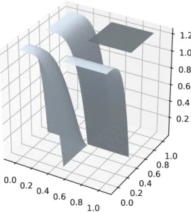
for some a, b, ω ∈ R. In the remaining of the section, we set a = 1/8, b = 3 and ω = 5. We show that Φ indeed defines an embedding. See Figure 8 for a plot of the submanifold M = Φ(T2). For an integer s≥ 1, we denote by Fs the density of the push forward measure Qs = Φ∗Gs⋅µT2 with
respect to the volume measure µM. Let x= (b+1, a, 0) be the image of 0 by Φ. Simple calculations show that the differential of Φ at 0 evaluated at e1= (1, 0) ∈ T0T2 and e2= (0, 1) ∈ T0T2 is equal to respectively dΦ(0)[e1] = 2π(aω, 0, 1) and dΦ(0)[e2] = 2π(0, b + 1, aω). Hence formula (17) yields
Figure 7: Plot of the probability density function Gs for s= 3.
Figure 8: Plot of the submanifold M (Left) for parameters a= 1/8, b = 3 and ω = 6, and 500 points sampled independently from Φ∗G
s⋅µT2 with s= 3 (Right). The black cross marks the point x. and we obtain Fs(x) = ( 2s + 4 2s + 3) 2 1 4π2((1 + a 2ω2) ((b + 1)2+a2ω2) − a2ω2)−12.
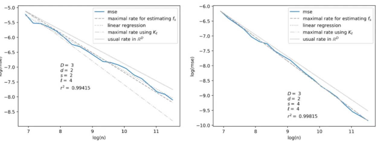
In the same way as in the previous section, we aim at providing an empirical measure for the rate of convergence of the risk R(p)n [ ̂fh, Ps] when h is suitably tuned with respect to n and s. This is done using again Algorithm 1. The results are presented in Figure 9.
5.3 Adaptation
In this section we estimate a density when its regularity is unknown, contrary to the previous simulation where the regularity parameter s is pugged in the bandwidth choice n−1/(2s+d). This is performed using Lepski’s method presented in Section 3.4. The MSE rate is computed using Algorithm 1, for both the one-dimensional and the two-dimensional synthetic datasets.
For the adaptive estimation on the two-dimensionnal manifold, we observed that the corrective term det dΦ(0) computed in (20) made the resulting density Fs(x) very small, while the function ψ
Figure 9: Plot of the empirical mean square error (blue) for a 2-dimensional submanifold with parameters s= 2, ℓ = 4 (Left) and s = 4, ℓ = 4 (Right). We use a log-regular grid n of 20 points ranging from 103
to 105
. Each experiment is repeated N= 500 times.
defined at (11) and used to tune the bandwidth soared dramatically because of the retained value of vd= 4dζd∥K(d,ℓ)∥2∞b, so that the values of ˆfh and ψ(h, ⋅) are not of the same order anymore at this scale (using maximum 106 observations). To circumvent this effect, we use a different kind of density gs,λ defined as
gs,λ(t) = Csλ(1 − (2λt)s+1) ✶[0,1/2λ](t) + Csλ(1 − (2λ(1 − t))s+2) ✶[1−1/2λ,1](t)
for some λ≥ 1 and with Cs= 1−1/(2s+2)−1/(2s+6). We plot the function gs,λ below in Figure10 for some value of s and λ= 2.
Figure 10: Plot of the probability density function gs,λ for λ= 2 and s ∈ {1, 3, 20}.
Again, gs,λ defines a probability density on T1 that is s-times differentiable at 0 but not s + 1-times. Like before, we consider the density Gs,λ ∶(t, u) ↦ gs,λ(t)gs,λ(u) on the torus T2 and the push-forwarded probability measure Φ∗Gs,λ⋅µT2 which has density Fs,λ with respect to µM. For λ= 10, we find that Fs,λ(x) ≃ 1 for most value of s, so that we set v = 1 in the definition of ψ for the sake of the estimation procedure. We have no theoretical guarantee that such a method work but we recover nonetheless the right rate in the estimation of the value of the density, see Figure 11. The numerical results are presented in Table1.
Figure 11: Plot of the empirical mean square error (blue) for s= 2, ℓ = 4 for a one-dimensional submanifold (Left) and a two-dimensional submanifold for s= 2 and ℓ = 3 (Right). The band-width h is chosen adaptively using Lepski’s method as in Section 3.4. Each experience is repeated N= 100 times.
D d ℓ s Choice of h 2s+D2s 2s+d2s 2ℓ+d2ℓ Linear regression Error (%)
2 1 4 2 Deterministic 0.667 0.8 0.889 0.759 5.08 2 1 4 4 Deterministic 0.8 0.889 0.889 0.851 4.25 3 2 4 2 Deterministic 0.571 0.667 0.8 0.602 9.65 3 2 4 4 Deterministic 0.727 0.8 0.8 0.798 2.48 2 1 4 2 Adaptive 0.667 0.8 0.889 0.756 5.65 3 2 3 2 Adaptive 0.571 0.667 0.75 0.630 5.55
Table 1: This table sums up the results of the simulation carried on in this section. In light blue is the expected rate for the mean square error. The column Linear regression contains the outcome of Algorithm1for the given set of parameters. We then compute the relative error between this coefficient and the expected rate in the last column.
6
Proofs
6.1 Proofs of Section 3.2
We set Kh(x) = h−dK(x/h) and start with bounding the variance of Kh(X−x) when X is distributed according to P ∈ Σsd. Let first observe that
∣Kh(X − x)∣ ≤ ∥ K∥∞
hd ✶BD(x,h)(X) ≤ ∥
K∥∞ hd Lemma 4. If P ∈ Σsd then, for all x∈ MP and all h≤ τ/2,
VarP(Kh(X − x)) ≤ v
hd where v= 4 dζ
d∥K∥2∞b. with ζd being the volume of the unit ball in Rd.
Proof. We have VarP(Kh(X − x)) ≤ EP[Kh(X − x)2] ≤ ∥ K∥2∞ h2d P(B(x, h)) ≤ 4dζdb∥K∥2∞ hd where we used (21) and Lemma 1with η= τ/2.
Using Bernstein inequality (Boucheron et al., 2013, Thm. 2.10 p.37), for any P ∈ Σsd, any x∈ MP, and any t> 0, we infer
P⎛ ⎝∣̂ξh(P, x)∣ ≥ √ 2vt nhd+ ∥ K∥∞t nhd ⎞ ⎠≤ 2e−t, (21)
where P is a short-hand notation for the distribution P⊗n of the n-sample X1, . . . , Xn taken under P. The bound (21) is the main ingredient needed to bound the Lp-norm of the stochastic deviation of ̂fh.
Proof of Proposition 4. We denote by y+ = max{y, 0} the positive part of a real number y. We start with
EP[∣̂ξh(P, x)∣p] ≤ 2p−1(v(h)p+ EP[(∣̂ξh(P, x)∣ − v(h))p +]) . The first term has the right order. For the second one, we make use of (21) to infer
EP[(∣̂ξh(P, x)∣ − v(h))p +] = ∫ ∞ 0 P(∣̂ξh(P, x)∣ > v(h) + u) pup−1du = pv(h)p ∫0∞P(∣̂ξh(P, x)∣ > v(h)(1 + u)) up−1du ≤ pv(h)p⎛ ⎝1+ ∫ ∞ 1 P⎛ ⎝∣̂ξh(P, x)∣ > √ 2v(1 + u) nhd + ∥ K∥∞(1 + u) nhd ⎞ ⎠up−1du⎞⎠ ≤ pv(h)p (1 + ∫1∞2e−1−uup−1du) ≤ pv(h)p(1 + Γ(p))
which ends the proof.
The proof of Lemma 2partly relies on the following technical lemma.
Lemma 5. Let β ≥ 1 be a real number and let g ∶ Rd → R verifying that ∥g∥∞ ≤ b and that the restriction of g to Bd(0, r) is β-H¨older, meaning that
∀v, w ∈ Bd(0, r), ∥dkg(v) − dkg(w)∥ ≤ R∥v − w∥δ
for some R≥ 0 with k = ⌈β − 1⌉ and δ = β − k. Then there exists a constant C (depending on β, r, b and R, and depending on β when r= ∞) such that, for all 1 ≤ j ≤ k,
sup v∈B(0,r/2)∥d
jg(v)∥
op≤ Cb1−j/βRj/β.
Proof. Let v∈ Bd(0, r/2). Since g is β-H¨older on Bd(0, r), we know that there exists a function Rv such that, for any z such that v+ z ∈ B(0, r), we have
g(v + z) − k ∑ j=0 1 j!d jg(v)[z⊗k] = R v(z)
with∣Rv(z)∣ ≤ R∥z∥β/k!. Let h = (2bk!/R)1/β, and z0∈ Rd be unit-norm. Pick a1, . . . , ak∈ (0, 1) all distincts and small enough such that hakz0∈ B(0, r/2) for all k (if r = ∞, then we can pick the ai independently from R, b and β). Introducing the vectors of Rk
X= (hdg(v)[z0], . . . , hk k!d kg(v)[z⊗k 0 ]) and Y = (g(v + ha1z0) − g(v) − Rv(ha1z0), . . . , g(v + hakz0) − g(v) − Rv(hakz0))
we have Y = V X with V being the Vandermonde matrix associated with the real numbers (a1, . . . , ak). The former being invertible, we have ∥X∥ ≤ ∥V−1∥op∥Y ∥ and thus, for any 1 ≤ j ≤ k
∣hj j!d jg(v)[z⊗k 0 ]∣ ≤ ∥V−1∥op(2b + R k!h β) .
Substituing the value of h and noticing that the former inequality holds for every unit-norm vector z0, we can conclude.
Proof of Lemma 2. We set Bh= BD(x, h). Since τ/4 is smaller than the injectivity radius of expx (see Proposition 2) we can write
fh(P, x) = ∫ Bh Kh(p − x) f(p)dµM(p) = ∫ exp−1 x Bh Kh(expxv− x)f(expxv)ζ(v)dv (22) with ζ(v) =√det gx(v). We set γ = α ∧ β and k = ⌈γ − 1⌉. Let F denote the map f ○ exp
x. For h smaller than (τ ∧ r)/4, we have exp−1x Bh ⊂ BTxM(0, 2h) ⊂ BTxM(0, (r ∧ τ)/2) (see Proposition 3).
We can thus write the following expansion, valid for all v∈ exp−1x Bh and all w∈ TxM, expx(v) = x + v + k+1 ∑ j=2 hj j!d j expx(0)[v⊗j] + R1(v) with ∥R1(v)∥ ≤ C1∥v∥γ+1, (23) F(v) = f(x) + k ∑ j=1 hj j!d jF(0)[v⊗j] + R 2(v) with ∣R2(v)∣ ≤ C2∥v∥γ, (24) K(v + w) = ✶{∥v+w∥≤1}⎛ ⎝K(v) + k ∑ j=1 hj j!d jK(v)[w⊗j] + R 3(v, w)⎞ ⎠ with ∣R3(v, w)∣ ≤ C3∥w∥γ, (25) with C1 depending on α, τ and L, C2 depending on β, r, b and R (see Lemma5), and C3 depending on K. Since now we know that gx
ij(v) = ⟨d expx(v)[ei], d expx(v)[ej]⟩, we have a similar expansion for the mapping ζ(v) =√det gx(v)
ζ(v) = 1 + k ∑ j=1 hj j!d jζ(0)[v⊗j] + R 4(v) with ∣R4(v)∣ ≤ C4∥v∥γ (26) with C4 depending on α, τ and L. Making the change of variable v= hw in (22), we get
fh(P, x) = k ∑ k=0
with Gj corresponding to the integration of the j-th order terms in the expansion around 0 of the function v↦ K (p−expp(hw)
h ) F(hw)ζ(hw). In particular Gj can be written as a sum of terms of the type
I = hj∫
1
hexp−1x Bh
dmK(w)[φ(w)⊗m]ψ(w)dw
where ψ and φ are monomials in w satisfying m deg φ+ deg φ = j, with coefficients bounded by constants depending on α, τ, L, β, r, b and R (again, use Lemma5 to bound the derivatives). Since now BTxM(0, 1) ⊂
1 hexp
−1
x Bh, and since djK is zero outside of B(0, 1), we have that Gjcan actually be written Gj(h, P, x) = hjG(P, x) with ∣G(P, x)∣ ≤ C for some C depending on K, α, τ, L, β, r, b and R. Similar reasoning leads to Rh(P, x) ≤ Chγ with C depending again on K, α, τ, L, β, r, b and R. To conclude, it remains to compute G0(P, x). Looking at the zero-th order terms in the expansions (23) to (26), we find that
G0(P, x) = ∫
BTxM(0,1)K(w)f(x)dw = f(x) where we used Assumption1. The proof of Lemma2is complete.
Proof of Proposition 5. For a positive integer ℓ ≥ 1, let fh(ℓ)(P, x) be the mean of the estimator ̂
fh(x) computed using K(ℓ). Let γ= α ∧ β and k = ⌈γ − 1⌉. We recursively prove on 1 ≤ ℓ < ∞ the following identity ∀h ≤ (τ ∧ r)/4, f(ℓ) h (P, x) = f(x) + k ∑ j=ℓ hjG(ℓ)j (P, x) + R(ℓ)h (P, x) (27)
where ∣R(ℓ)h (P, x)∣ ≤ C(ℓ)hγ for some constant C(ℓ) depending on τ, ℓ, L, R, b, β and r. The initial-isation step ℓ= 1 has been proven in Lemma 2. Let now 1≤ ℓ ≤ k. By linearity of fh(P, x) with respect to K, we have
fh(ℓ+1)(P, x) = 2f2(ℓ)−1/ℓh(P, x) − fh(ℓ)(P, x). Since 2−1/ℓh≤ h, we can use our induction hypothesis (27) and find
fh(ℓ+1)(P, x) = f(x) + k ∑ j=ℓ (21−j/ℓ− 1)hjG(ℓ) j (P, x) + 2R (ℓ) 2−1/ℓh(P, x) − R (ℓ) h (P, x).
We conclude noticing that 21−j/ℓ− 1 = 0 for j = ℓ, and setting G(ℓ+1)j (P, x) = (21−j/ℓ− 1)G(ℓ)j (P, x) and R(ℓ+1)h (P, x) = 2R(ℓ)2−1/ℓh(P, x) − R(ℓ)h (P, x). The new remainder term verifies
∣R(ℓ+1)
h (P, x)∣ ≤ (2
1−γ/ℓ+ 1)C(ℓ)hγ≤ 3C(ℓ)hγ
(28) ending the induction by setting C(ℓ+1)= 3C(ℓ). When ℓ≥ k + 1, the induction step is trivial.
6.2 Proofs of Section 3.3
We go along a classical line of arguments, thanks to a Bayesian two-point inequality by means of Le Cam’s lemma (Yu,1997, Lem. 1), restated here in our context. For two probability measures P1, P2, we write TV(P1, P2) = supA∣P1(A) − P2(A)∣ for their variational distance and H2(P1, P2) = ∫ (√dP1−√dP2)
2
Lemma 6. (Le Cam) For any P1, P2∈ Σα,β(x), we have, inf ̂ f R (p) n [ ̂f ,Σα,β](x) ≥ 1 2∣f1(x) − f2(x)∣ (1 − TV (P ⊗n 1 , P2⊗n)) (29) ≥ 1 2∣f1(x) − f2(x)∣ (1 − √ 2− 2(1 − H2(P 1, P2)/2)n) .
Proof. The proof of (29) can be found in Yu (1997, Lem. 1). It only remains to see that TV(P1⊗n, P2⊗n) ≤√2− 2(1 − H2(P
1, P2)/2)n. This comes from classical inequalities on the Hellinger distance, see Tsybakov(2008, Lem. 2.3 p.86) and Tsybakov(2008, Prp.(i)-(iv) p.83).
Proof of Theorem 2. Suppose without loss of generality that x= 0 and consider a smooth submani-fold M of Rd+1⊂ RD that contains the disk B
d(0, 1) ⊂ Rdwith reach is greater than τ , see Figure12 for a diagram of such an M . By smoothness and compacity of M , there exists L∗ (depending on τ) such that M ∈ Cd,α(τ, L∗). Let P be the uniform probability measure over M, with density f ∶ x ↦ 1/ vol M. We have P ∈ Σα,β(0) as long as L∗ ≤ L and a ≤ 1/ vol M ≤ b an assumption we make from now on. For 0< δ ≤ 1, let Pδ= fδ⋅µM with
fδ(y) =⎧⎪⎪⎨⎪⎪ ⎩
f(y) + δβG(y/δ) if y ∈ B(0, δ) f(y) otherwise
with G ∶ Rd→ R a smooth function with support in Bd(0, 1) and such that ∫RdG(y)dy = 0. We
pick G such that fδ ∈ Fβ for small enough δ, depending on r and τ . Such a G can be chosen to depend on R only.
Figure 12: Diagram of a candidate for M (Left) and of the densities f and fδ around 0 (Right).
For δ small enough (depending on r and τ ), we thus have Pδ ∈ Σα,β(0) as well. By Lemma 6, we infer inf ̂ f R (p) n [ ̂f ,Σα,β](0) ≥ 12δβ∣G(0)∣ (1 − √ 2 − 2(1 − H2(P, P δ))n) so that it remains to compute H2(P, P
δ). We have the following bound H2(P, Pδ) = ∫ Bd(0,δ) (1 −√1 + vol M δβG(x/δ))2dx ≤ ∫B d(0,δ)(vol M) 2δ2βG2(x/δ)dx ≤ (C ∨ 1)δ2β+d
with C = vol M ∫B(0,1)G(x)2dx depending on τ and R only. Taking γ = (1/(C ∨ 1)n)1/(2β+d) we obtain, for large enough n (depending on τ )
inf ̂ f R (p) n [ ̂f ,Σα,β](0) ≥ 12((C ∨ 1)n) −β/(2β+d)√ 2− 2(1 − 1/n)n≥ C ∗n−β/(2β+d),
with C∗= (C ∨ 1)−1/2depending on τ and R.
6.3 Proofs of Section 3.4
Lemma 7. For any p≥ 1, P ∈ Σsd(x), and D2> p, we have R(p)
n [ ̂f , P](x) ≲ v(h∗(P, x))λ(h∗(P, x)) up to a constant depending on p, D1 and D2, with
h∗(P, x) = max {h ∈ H ∣ ∀η ∈ H(h), ∣fη(P, x) − f(x)∣ ≤ D1v(h)λ(h)}.
Proof. We fix P ∈ Σα,β(x) and write ̂h and h∗for ̂h(x) and h∗(P, x) respectively. Let A = {̂h ≥ h∗}. We can write(R(p)n [ ̂f , P](x))
p
= RA+ RAc, where
RA= EP[∣ ̂f(x) − f(x)∣p✶A] and RAc= EP[∣ ̂f(x) − f(x)∣p✶Ac].
We start with bounding RA. Firstly,
RA≤ 3p−1(EP[∣ ̂f̂h(x) − ̂fh∗(x)∣p✶A] + EP[∣ ̂fh∗(x) − fh∗(P, x)∣p✶A]
+ EP[∣fh∗(P, x) − f(x)∣p✶A]).
Next, by definition of ̂h andA, we have
∣ ̂f̂h(x) − ̂fh∗(x)∣✶A≤ ψ(̂h, h∗)✶A≤ (2D1+ 2)v(h∗)λ(h∗).
By definition of h∗, we also have ∣fh∗(P, x) − f(x)∣ ≤ D1v(h∗)λ(h∗). Finally, using Proposition4
EP[∣ ̂fh∗(x) − fh∗(P, x)∣p✶A] ≤ cpv(h∗)p≤ cp(v(h∗)λ(h∗))p
holds as well. Putting all three inequalities together yields
RA≤ CA(v(h∗)λ(h∗))p with CA= 3p−1((2D1+ 2)p+ cp+ D1p) . We now turn to RAc. Notice that for any h∈ H(h∗), we have
∣fh(P, x) − f(x)∣ ≤ D1v(h∗)λ(h∗) ≤ D1v(h)λ(h), hence
∣ ̂fh(x) − f(x)∣ ≤ D1v(h∗)λ(h∗) + ∣̂ξh(P, x)∣. We can thus write
RAc = ∑ h∈ ˚H(h∗) EP[∣ ̂fh(x) − f(x)∣p✶ {̂h=h}] ≤ ∑ h∈ ˚H(h∗) EP[(D1v(h∗)λ(h∗) + ∣̂ξh(P, x)∣])p✶ {̂h=h}].
Now, for any h∈ H, h < h∗, we have
{̂h = h} ⊂ {∃η ∈ H(h), ∣ ̂f2h(x) − ̂fη(x)∣ > ψ(2h, η)} ⊂ ⋃
η∈H(h)
{2D1v(h∗)λ(h∗) + ∣̂ξ2h,η(P, x)∣ > ψ(2h, η)} ,
where ̂ξ2h,η(P, x) = ̂ξ2h(P, x)−̂ξη(P, x), and where we used the triangle inequality and the definition of h∗. Now, we have 2D1v(h∗)λ(h∗) ≤ 2D1v(2h)λ(2h) since 2h ≤ h∗ and by definition of ψ(2h, η), we infer {̂h = h} ⊂ ⋃ η∈H(h){∣̂ξ 2h,η(P, x)∣ > v(2h, η)λ(η)} so that P(̂h = h) ≤ ∑ η∈H(h) P(∣̂ξ2h,η(P, x)∣ > v(2h, η)λ(η)) (30) ≤ ∑ η∈H(h) P⎛ ⎝∣̂ξ2h,η(P, x)∣ > √ 8vλ(η) nηd + 2∥K∥∞λ(η) nηd ⎞ ⎠ ≤ ∑ η∈H(h) 2 exp(−λ(η)2). (31)
For (30) we use the fact that λ(η) ≥ 1 and Bernstein’s inequality on the random variable ̂ξ2h,η(P, x) for (31). Noticing now that λ(η)2≥ dD
2log(h+/η), we further obtain P(̂h = h) ≤ 2 (h h+) D2d ×⌊log2(h +/h−)⌋ ∑ j=0 2−jD2d≤ 2 1− 2−D2d( h h+) D2d .
For any h∈ H, h < h∗, we thus get the following bound, using Cauchy-Schwarz inequality EP[(D1v(h∗)λ(h∗) + ∣̂ξh(P, x)∣]) p ✶{̂h=h}] ≤ P(̂h = h)1/2E P[(D1v(h∗)λ(h∗) + ∣̂ξh(P, x)∣]) 2p ]1/2 ≤ 2(2p−1)/2 √ 2 1− 2−D2d( h h+) D2d/2 (Dp 1v(h ∗)pλ(h∗)p+ c1/2 2p v(h) p) . (32) We plan to sum over h∈ ˚H(h∗) the RHS of (32). Notice first that
∑ h<h∗
hD2d/2≤ (h∗)D2d/2(1 − 2−D2d/2)−1.
Moreover, for any h≥ h−, we have v(h) ≤ 2√2v/(nhd) by definition of h−. It follows that v(h∗) ≤ v(h) ≤ 2v(h∗) (h
∗ h )
d/2 . for any h≤ h∗. This enables us to bound the following sum
∑ ˚ H(h∗) hD2d/2v(h)p≤ 2pv(h∗)(h∗)pd/2 ∑ ˚ H(h∗) hD2d/2−pd/2 ≤ 2p 1− 2(p−D2)d/2v(h ∗)(h∗)D2d/2
where we used that D2> p. Putting all these estimates together, using that h∗/h+≤ 1 and λ(h∗) ≥ 1, we eventually obtain RAc ≤ CAcv(h∗)pλ(h∗)p with CAc= 2 p √ 1− 2−D2d( D1p 1− 2−D2d/2+ √c 2p2p 1− 2(p−D2)d/2) .
In conclusion (R(p)n [ ̂f(x), P])p≤ (CA+ CAc)v(h∗)pλ(h∗)p which completes the proof.
Proof of Theorem 3. Let P ∈ Σα,β(x) and let ¯h = (ω log n/n)1/(2γ+d) with γ = α ∧ β and for some constant ω to be specified later. By Proposition5 we know that for n large enough (depending on ω, α, β, d) such that ¯h≤ (r ∧ τ)/4, we have ∣fη(P, x) − f(x)∣ ≤ C1ηγ for all η≤ ¯h with C1 depending on K, ℓ, α, τ, L, β, r, b and R. Moreover, we also have
D21v(¯h)2λ(¯h)2 C2 1¯h2γ ≥ D12dD22v log(1/¯h) C2 1n¯h2γ+d = D21dD22v(2γ + d)−1 C2 1ω
log n− log log n − log ω
log n .
Thus, picking ω= D2
1dD2v(2γ + d)−1/C12 yields C1¯hδ ≤ D1v(¯h)λ(¯h) for n large enough (depending on ω), and therefore ¯h≤ h∗(P, x). By Lemma 7this implies
R(p)
n [ ̂f , P](x) ≤ C2v(¯h)λ(¯h)
where C2 depends on p, D1 and D2. But using that both ¯h ≥ h− and λ(¯h)2 = dD2log(1/¯h) for n large enough (depending on ω, d, K and D2), we also obtain
v(¯h)2λ(¯h)2≤ 8vdD2log(1/¯h) n¯hd =
8vdD2(2γ + d)−1 ω
log n− log log n − log ω log n ¯h
2γ≤ 8C12 D12
¯ h2γ.
This last estimate yields R(p) n [ ̂f(x), P] ≤ ( 4C1C2 D1 ωγ/(2γ+d)) (log n n ) γ/(2γ+d)
for n large enough depending on ω, α, β, d, K and D2, which completes the proof.
6.4 Proofs of Section 3.5
Proof of Proposition 6. Let P ∈ Σdα,β(x) and η > 0. Assume that ̂Pη > 0. We have ∣̂δη− d∣ ≤
1
log 2∣ log ̂P2η− log ̂P2η∣ + 1
log 2∣ log ̂Pη− log ̂Pη∣ + 1
log 2∣ log ̂P2η− log Pη− d log 2∣ ≤ 1 log 2(∣ ̂ P2η− P2η∣ ̂ P2η∧ P2η + ∣P̂η− Pη∣ ̂ Pη∧ Pη + ∣log (P2η/(2dPη))∣)
We first consider the determinist term. For η ≤ τ/2, we have, writing rη = ξ(η/τ)η and using Lemma1,
L2η(1 − η2/6τ2)(2η)2ζd≤ P2η≤ U2η(1 + r2η2 /τ2)rd2ηζd and