A watershed scale study of climate change impacts on
groundwater recharge
(Annapolis Valley, Nova Scotia,
Canada)
Étude des impacts des changements climatiques sur la
recharge à l’échelle d’un bassin versant (vallée d’Annapolis,
Nouvelle-Écosse, Canada)
Christine Rivard1*, Claudio Paniconi2, Harold Vigneault2 and Diane Chaumont3
1 Geological Survey of Canada, Quebec City, Qc, Canada
2 INRS, Centre Eau Terre Environnement, Quebec City, Qc, Canada 3 Ouranos Inc., Montréal, Qc, Canada
* Corresponding author: [email protected]
Abstract The potential impacts of future climate change on the evolution of groundwater recharge
are examined at a local scale for a 546 km2 watershed in eastern Canada. Recharge is estimated
using the infiltration model HELP with inputs derived from five climate runs generated by a regional climate model in combination with the A2 greenhouse gas emissions scenario. The model runs project an increase in annual recharge over the 2041-2070 period. On a seasonal basis, however, a marked decrease in recharge during the summer and a marked increase during the winter is observed. The results suggest that increased evapotranspiration resulting from higher temperatures does not offset the large increase in winter infiltration. In terms of individual water budget components, marked differences are obtained for the different climate change scenarios. Monthly recharge values are also found to be quite variable, even for a given climate scenario. These findings are compared with results from two regional scale studies.
Résumé: Les impacts potentiels des changements climatiques sur l’évolution de la recharge ont été
étudiés à l’échelle locale, sur un bassin versant de 546 km2 dans l’est du Canada. La recharge a été
évaluée en utilisant le modèle d’infiltration HELP et cinq scénarios climatiques issus d’un modèle régional climatique, en combinaison avec le scénario de gaz à effet de serre A2. Les simulations prédisent une augmentation de la recharge annuelle sur la période 2041-2070. Sur une base mensuelle cependant, une diminution marquée de la recharge durant l’été et une augmentation marquée en hiver sont observées. Les résultats suggèrent que l’augmentation de l’évapotranspiration résultant des températures plus élevées ne compense pas l’importante augmentation des infiltrations hivernales. Les différentes composantes du bilan hydrique montrent des différences importantes d’un scénario à l’autre. La recharge mensuelle s’avère également assez variable, même pour un scénario climatique donné. Ces conclusions sont comparées avec les résulats de deux études à l’échelle régionale.
Key words recharge, climate change, infiltration model, Annapolis Valley (Canada)
Mots-clés recharge, changements climatiques, modèle d’infiltration, vallée d’Annapolis (Canada)
Accepted Manuscript
1. INTRODUCTION
Groundwater recharge can be defined as the amount of water that percolates downward by gravity through the unsaturated zone and reaches the water table. Reliable information on this state variable is essential for the sustainable management and protection of aquifers. Recharge rates are governed by geology (including soil properties), land surface features (including topography, land cover, and land use), and climate (atmospheric forcing). Assessing climate change impacts on aquifer recharge is not straightforward due to the complexity of the processes and interactions involved, and to date, relatively few studies have been devoted to this topic. Moreover, as underscored by Arnell et al. (2001), the effect of climate change on groundwater recharge varies greatly between regions and between climate scenarios. Identifying periods when water is expected to be more abundant and predicting periods of water scarcity is an essential step towards climate change adaptation. This type of assessment can be carried out by running hydrological models with various climate scenarios generated using climate models and greenhouse gas (GHG) emissions scenarios.
Eckhardt and Ulbrich (2003) studied a 693 km2 catchment in Germany using a modified version of the agronomic land surface model SWAT and climate change scenarios from the European ACACIA project for the A2 (high) and B1 (low) GHG emissions scenarios. Similar results were obtained for the two scenarios, although with stronger impacts for the A2 case. They found that the impacts of climate change on groundwater recharge and streamflow were small on an annual basis. They attributed this result mainly to the fact that increased atmospheric CO2 levels reduce stomatal conductance, thus counteracting the increasing potential evapotranspiration induced by rising temperatures and decreasing precipitation. More pronounced changes were found on a seasonal basis: winter recharge increased due to earlier snowmelt and summer recharge decreased by up to 50%.
Jyrkama and Sykes (2007) used the infiltration model HELP and statistically downscaled climate data from global climate models (GCMs) provided in the IPCC Third Assessment Report for a 7000 km2 rural watershed in southwestern Ontario (central Canada). They found that, on an annual basis, recharge rates would increase
Accepted Manuscript
as a result of climate change for all eight simulated scenarios, from 10% to 53%. Similar to Eckhardt and Ulbrich (2003), they observed earlier snowmelt and an increased recharge during the winter as a result of the higher rain/snow ratio.
Toews and Allen (2009) modeled a 194 km2 irrigated region in the Okanagan Valley (western Canada), also with the HELP model and with climate projections generated by three GCMs for the A1 and A2 emissions scenarios. Their main conclusion was that the prediction of future recharge is highly dependent on the selected GCM model. Small increases of recharge were observed on an annual basis, and again earlier peak winter recharge was projected as well as lower recharge rates and higher potential evapotranspiration for the summer months.
Sulis et al. (2011) studied climate change impacts for a 690 km2 watershed in the southern part of Quebec (Canada) using the coupled surface/subsurface model CATHY and one climate projection from a regional climate model for the A2 GHG emissions scenario. The results showed that the complexities of rainfall-runoff-infiltration partitioning lead to important variations in the response of streamflow to climate change, especially during the summer. As with other studies, these authors also found that recharge would increase subtantially during the winter.
Stoll et al. (2011) and Goderniaux et al. (2011) also used coupled integrated surface/subsurface models (MIKE SHE and HydroGeoSphere, respectively) to study potential impacts of climate change on groundwater for small to moderate-size catchments (9 km2 and 480 km2). Stoll et al. (2011) used 8 GCM/RCM (global/regional climate model) combinations and concluded that the downscaling process was an important source of uncertainty in hydrological impact studies. They recommended that downscaling techniques be verified before applying them to climate model data. Goderniaux et al. (2011) used a stochastic weather generator to obtain 30 transient climatic scenarios for each of six different RCMs. They showed that the climate change signal becomes stronger than that of natural climate variability by 2085.
Although eastern Canada does not have a water deficit (the potential evapotranspiration in this region is not higher than total precipitation), reliable
Accepted Manuscript
information on the trends and probable impacts of future climate change is crucial to planning adequate adaptation, mitigation, and protection measures that will ensure sustainable management of water resources. In this paper, five climate projections generated from the fourth version of the Canadian Regional Climate Model (CRCM4) (de Elía and Côté, 2010; Caya and Laprise, 1999) and the A2 gas emissions scenario are used to drive the infiltration model HELP (Schroeder et al., 1994) in simulations to evaluate the effects of climate change on aquifer recharge as well as the sensitivity of various water budget components to climate data. The study area is a 546 km2 watershed situated in the Annapolis Valley, Nova Scotia, one of the major fruit growing regions of Canada. A second objective of this paper is to compare the results obtained from this comparatively small (local) scale modeling study with those from two recent regional scale studies of aquifer recharge, one based on different recharge estimation approaches, including modeling (Rivard et al., 2013), and the other on historical records of baseflow and well hydrographs (Rivard et al., 2009). In the former study, five regional recharge assessment approaches were used, including river hydrograph separation, river low flows, a water budget, a hydrogeological model (FEFLOW), and a hydrological model (HELP). HELP was found to be an adequate tool for recharge estimation compared to the other methods. In the latter study, decreasing statistical trends in recharge over the last decades were found for the Maritimes region in eastern Canada using the trend-free pre-whitening method based on the Mann-Kendall test.
The HELP model has been used in previous studies, as described above, for analyzing climate change impacts on groundwater recharge. It is well suited to this purpose as it is a computationally efficient yet comprehensive model of hydrological processes across the atmosphere-soil-vegetation continuum. Nonetheless the model also has its limitations (see for e.g. Guay et al., 2013); for instance, it does not account for processes such as reinfiltration (no interaction between adjacent model cells) and deep groundwater flow (the model only simulates water movement down to the water table and thus assumes unconfined conditions). This model should thus be regarded as one of many possible modeling approaches for studying hydrological climate change impacts. The A2 emissions scenario used in this study is one of the scenarios that follows most closely recent observed emissions trends (Raupach et al., 2007). The five climate projections selected are driven by five different members of the Canadian
Accepted Manuscript
Coupled Global Climate Model (CGCM3) (Scinocca et al, 2008) and provide a range of plausible future climate differentiated by natural variability (the five members of CGCM3 differ only in their initial conditions). Regional climate models, such as CRCM4, are especially well adapted to climatic conditions such as those found in the study area, which is located along the coast and is subject to local valley effects. 2. DESCRIPTION OF THE STUDY AREA
2.1 General context
The Annapolis Valley is a long (100 km) and narrow (10-15 km) lowland along the south shore of the Bay of Fundy in Nova Scotia (eastern Canada). The region, including part of the surrounding mountains, extends over 2 100 km2 and comprises five watersheds (Figure 1). The study area used for this paper corresponds to the drainage area of the Environment Canada gauging station 01DC005. It covers 546 km2, i.e., 34% of the Annapolis watershed (see Figure 1). Based on available data, this catchment is considered to be representative of the entire Valley in its geology, topography, land use, and vegetation cover. Topographic elevation in the South and North Mountains bounding the valley rarely exceeds 250 m above sea level (ASL).
The Annapolis Valley is a major economic region of the province and its most important agricultural area. More than 90% of the Valley residents rely on groundwater for domestic purposes, either from municipal wells or from private residential wells. On a regional scale, groundwater withdrawals do not present particular problems (Rivard et al., 2012).
Average annual total precipitation in the region is 1120 mm, and between 15% and 25% of this precipitation falls as snow. Monthly average temperatures range from -5 to +19oC (Environment Canada, http://climate.weatheroffice.gc.ca/climate_normals/index_e.html). The Valley has slightly warmer average temperatures, lower precipitation, and more frost-free days than the surrounding highland areas. The Greenwood weather station, located in the middle of the watershed (see Figure 1), provides representative data and the longest meteorological time series for the region.
Accepted Manuscript
2.2 Geological and hydrogeological contexts
The Valley includes sedimentary rocks of the Wolfville Formation and the overlying Blomidon Formation along its northern boundary. It is flanked to the south by South Mountain (South Mountain Batholith), composed of Paleozoic rocks, containing mainly granitic and metasedimentary rocks (slate, shale, siltstone, and quartzite) from the Meguma group and the Annapolis Supergroup (undifferentiated Lower Paelozoic unit in Figure 2). North Mountain is composed of basaltic rocks of the North Mountain Formation (Figure 2). The Wolfville, Blomidon, and North Mountain formations are Mezosoic rocks that belong to the Triassic-Jurassic Fundy Group (Hamblin, 2004). Figure 3 shows a conceptual model of the study area at the regional scale.
The main bedrock aquifers of the Valley are located in the Wolfville and Blomidon formations and, to a lesser extent, in the North Mountain basalts. The Wolfville and Blomidon formations are composed of lenticular bodies of sandstone, conglomerate, shale, and siltstone. The Wolfville Formation is typically dominated by coarser-grained facies, whereas the Blomidon Formation, located at the foot of North Mountain, is characterized by more fine-grained strata. Median hydraulic conductivities (K) of the Wolfville, Blomidon and North Mountain formations are, respectively, 6.2 x 10⁻⁶, 2.8 x 10⁻⁶, and 5.2 x 10⁻⁷ m/s, based on pump test results from the provincial database.
The Quaternary sediments in the study area consist mostly of glacial tills. Ice-contact glaciofluvial sands and gravels are also present in the eastern part of the Valley, as well as glaciomarine and/or glaciolacustrine sediments, mainly north of the glaciofluvial deposits. Permeameter tests have provided mean values of hydraulic conductivities ranging between 10-7 to 10-4 m/s. The sediment cover is usually quite thin (0-10 m), but it can reach 30 m in the sand and gravel units. Because there was not enough stratigraphic information in the Quaternary sequence to build a meaningful conceptual model of the sediment cover, the top layer was defined using the different sediment types derived directly from the surficial geology map, without any stratigraphy, except for a basal till layer that was assumed present throughout the
Accepted Manuscript
study area over the bedrock, based on the expected stratigraphic sequence for the region.
Groundwater levels have a median depth of 6.1 m; they are therefore found either within surficial sediments or bedrock. Although confined conditions are common in the Valley, due to an overlying grained sediment cover or to a fine-grained rock layer above the aquifer unit, groundwater flow seems to mainly follow topography, based on piezometric data (Rivard et al., 2012).
3. MATERIAL AND METHODS 3.1 The infiltration model
HELP (Hydrologic Evaluation of Landfill Performance) is a quasi-2D physically-based hydrological model (Schroeder et al., 1994). It simulates water movement down to the water table accounting for the effects of surface storage, snowmelt, surface runoff, infiltration, evapotranspiration (ET), vegetative growth, soil moisture storage, lateral subsurface drainage, and unsaturated vertical drainage. HELP is a commonly used diagnostic model for the estimation of recharge, in which ET is based on the Penman equation (Penman, 1963), incorporating wind and humidity effects as well as long wave radiation losses, root depth, growing season, and leaf area index (LAI). HELP uses some empirical relationships; it has been shown to work well in humid areas.
The HELP model has been previously implemented and calibrated for the Annapolis Valley using current-day conditions (Rivard et al., 2013). This section therefore provides only an overview of the model setup and assigned parameter values. Cells of 250 m × 250 m were selected to obtain a good compromise between spatial coverage (using mean values for the data representation), computing time, and available data for the different variables. ArcGIS was used to create each layer and to assign parameter values to each cell. An automated program was developed in C++ to allow all the cells (6741) to be run in batch mode so that the entire study area could be simultaneously considered (although without hydraulic connection between them). Each cell is discretized vertically into 1 to 4 layers, with each layer representing a
Accepted Manuscript
geological unit with homogeneous properties. A single layer is used when bedrock is outcropping; four layers are used only when two bedrock formations are encountered, such as at the Blomidon/Wolfville contact; most cells however have two (e.g. till, then bedrock) or three (e.g. sand, basal till, then bedrock) layers. The bottom of the cell corresponds to the groundwater level (depth), which may not necessarily correspond to the water table if the aquifer is confined.
Data related to climate, soil and rock physical properties, topography, land use, and vegetation cover and growth period were integrated into the model. Daily climate inputs consist of total precipitation (Ptot) and mean temperature (Tmean), which were taken from the Environment Canada National Climate Data and Information Archive (http://climate.weatheroffice.gc.ca/Welcome_e.html?&) for the Greenwood station, as well as daily solar radiation data that were generated by the model using Ptot and latitude. Mean annual wind speed and mean seasonal relative humidity, also taken from the Environment Canada archive for the Greenwood station, were integrated into the model as well. The mean annual wind speed is 15.3 ± 5.7 km/h, while the mean relative humidity values are 77, 71, 74 and 77% from winter to autumn.
Required subsurface physical properties are hydraulic conductivity (K), total porosity (n), wilting point, and field capacity. Average root depth for the dominant vegetation (plant, tree, or crop) over each cell, determined using a land use map, and vegetation growth period, determined based on the professional judgment of an Environment Canada agronomist, were also provided. K and some total porosity values were obtained from fieldwork and analyses performed during a regional characterization study (Rivard et al., 2012). The remaining parameters were assigned to geological formations or sediment classes (presented in Table 1) according to the
literature (Todd, 1980 and university websites
(http://www.terragis.bees.unsw.edu.au/terraGIS_soil/sp_water-soil_moisture_classification.html; http://www.extension.umn.edu/distribution/cropsystems/DC7644.html) Slope classes were selected based on the digital elevation model (DEM) for the region. Curve numbers from the SCS method, modified by Monfet (1979) for eastern Canada conditions, were used. These curves allow the prediction of surface runoff using rainfall-runoff
Accepted Manuscript
relations based on a combination of soil, soil cover, hydrologic conditions, and slope values. Table 1 presents the physical parameter values used in the calibrated model.
The precipitation and temperature data used for this present study consist of climate forecasts generated from a climate model (see below). Solar radiation is generated by HELP based on daily precipitation and latitude. All other variables related to climate and vegetation (relative humidity, wind speed, LAI, root depth, growing season duration) were kept constant for the future period since no data is currently available to adjust them, and since their impact on the model response appears to be limited compared to precipitation and temperature (see Rivard et al. (2013) and section 4.2 below). This is consistent with other studies, for instance McCallum et al. (2010), who found, in a sensitivity analysis of climate change on recharge, that recharge is most sensitive to change in precipitation, and, to a lesser extent, temperature and rainfall intensity.
3.2 Climate scenarios: climate model and emissions scenario 3.2.1 A2 greenhouse gas emissions scenario
The IPCC assessment reports (IPCC, 2007) constitute the most widely accepted scientific basis on climate evolution. The IPCC Special Report on Emissions Scenarios (SRES; Nakicenovic et al., 2000) first presented the SRES scenarios, which
are grouped into four families (A1, A2, B1, and B2; see
http://www.grida.no/publications/other/ipcc_tar/?src=/CLIMATE/IPCC_TAR/WG1/029.htm) that explore alternative development pathways covering a wide range of demographic, economic, and technological driving forces and associated GHG emissions (IPCC, 2007).
The selected SRES scenario for the present study is A2. This scenario describes a heterogeneous world with high population growth, limited reserves of oil and gas, slow economic development, and slow technological change with regards to efficient technologies. Based on recent available data, this scenario appears to be close to the observed emissions, along with the A1 family (Raupach et al., 2007).
Accepted Manuscript
3.2.2 Canadian Regional Climate Model
Regional climate models allow the transfer of large-scale information from their host GCMs to scales that are closer to the river basin or watershed scale. Compared to global climate models, the enhanced horizontal resolution obtained via the dynamical downscaling performed by an RCM results in a more accurate discretization of equations that generally leads to an improvement of the representation of surface forcings, such as those due to topography, large lakes, and coastal regions [Giorgi and Marinucci, 1996].
The fourth version of the Canadian Regional Climate Model (de Elía and Côté, 2010; Caya and Laprise, 1999) used in this study was driven by the third generation of the Canadian Coupled Global Climate Model (CGCM3) (Scinocca et al, 2008) being developed by the Canadian Center for Climatic Modeling and Analysis (CCMA). CGCM3 has four main components: a general atmospheric circulation model (with 31 vertical levels), a general ocean circulation model, an ice-sea thermodynamic model, and a soil-vegetation model. The spatial resolution is 3.75 degrees of latitude/longitude. The CRCM runs were produced by the Ouranos consortium over a domain covering North America (AMNO) with a spatial resolution of 45 km × 45 km (compared to 400 km × 400 km for GCMs).
The climate scenarios used in this study are based on five climate simulations performed with CRCM4 driven by different members of CGCM3 resulting from different initial conditions (see Table 2). All simulations were obtained with the A2 GHG emissions scenario. In order to compare projected climate changes with a “past” scenario having the same characteristics as those collected by weather stations, 30-y series for a reference and a future period were used, both generated by CRCM4. The 30-year time series used in this study correspond to the 1971-2000 period, the one currently used by Environment Canada for its climate normals, and the 2041-2070 period. Climate data from the five climate scenarios are considered equally probable. Thiessen polygons were used to allocate percentages to the different 45 km × 45 km
tiles, with four tiles providing coverage of the 01DC005 watershed (Figure 4). Using five different realizations of a single GCM to run a single RCM results in a narrower coverage of future plausible climate in comparison to using five different GCM/RCM
Accepted Manuscript
combinations. Nonetheless, considering the coastal environment of the region, RCM simulations were more appropriate and the CRCM4 runs were the only regional climate projections over eastern Canada available to us at the time of the study. Moreover, the CRCM4 model is well adapted to Canadian conditions and the model has been rigorously tested at Ouranos for various configurations throughout North America (de Elía and Côté, 2010).
Figure 5 presents box plots for the annual total precipitation (Ptot) and minimum temperature (Tmin) generated by CRCM4 for the five climate scenarios over both 30-y periods, as well as observation data for comparison. The CRCM4 model reproduces well the maximum temperature (Tmax) (not shown) of the past period, but it underestimates Tmin (and so also the mean temperature Tmean, which is the average of Tmax and Tmin), thus simulating a cooler climate. In Figure 5b it can be observed that historical values (observations) of Tmin are closer to synthetic values of the future period. On an annual basis over the period 1971-2000, observations for Tmean give an average of 6.77±0.74˚C, while synthetic past values yield 5.22±0.75˚C on average for the five scenarios. Future CRCM values for the 2041-2070 period produce an annual average of 8.19±0.89˚C.
Monthly differences between observations and results from the five members (individually) for the past period range from -2.1 to 1.2˚C for Tmax and from -6.5 to -0.1˚C for Tmin, resulting in a general underestimation of -4.2˚C to 0˚C for Tmean, the largest differences occurring during the winter (especially January and February). For total precipitation, synthetic annual values for the past period (1145±108 mm/y on average for the five scenarios) are generally similar to observations (1121±130 mm/y), with a difference of less than 5% for all climate runs. However, on a monthly basis, variations may be important, ranging from up to 39% (overestimation in June for the adl scenario) to -29% (underestimation in January, also for the adl scenario) over the five scenarios. The spring and summer seasons are, on average, overestimated by CRCM4 (by 12% and 22%, respectively), while autumn and winter are slightly underestimated (by 10%).
Figure 6 provides a comparison between a past scenario afa and observations for monthly values of Tmean and Ptot over the 30-y period. The other four climate
Accepted Manuscript
simulations show similar behavior. The mild winters and the precipitation patterns particular to the Valley do not appear to be well simulated, mainly due to the relatively large tiles of CRCM that make it difficult for the model to capture some of the micro-climate features of the study region. Table 3 presents annual and seasonalvalues averaged over the five scenarios for the past period, as well as observations for comparison (winter: Dec, Jan, Feb; spring: Mar, Apr, May; summer: Jun, Jul, Aug; autumn: Sep, Oct, Nov).
Figure 7 illustrates the monthly differences between future and past periods averaged over 30 years for the five scenarios for Tmean and Ptot, the two variables used in HELP. Each month (for each individual scenario) has a difference varying from -21.7 to +42.1 mm/y for Ptot and from 1.0 to 5.8˚C for Tmean. For both variables, the largest differences occur during winter while the smallest are projected for summer and beginning of autumn. These differences between the two periods are much smaller than the variations (standard errors) associated with a given scenario over 30 years, which are of the same order of magnitude for both climate change and the baseline scenarios. Projected changes for annual Tmean derived from CCCma/CGCM3 simulations for the A2 GHG emissions scenario fall within the range 1.5 to 4˚C for this area and the 2041-2070 period (http://www.cccma.ec.gc.ca/diagnostics/cgcm3-t47/cgcm3.shtml).
3.2.3 The delta change method
The commonly used delta change (or perturbation) method (van Roosmalen et al., 2009; Jackson et al., 2011; Sulis et al., 2011) was used in this study to generate the climate change scenarios since the CRCM outputs did not always reproduce well the monthly observed records, especially for precipitation (e.g., Figure 6). The mean monthly differences between values from the future and past periods averaged over 30 years (shown in Figure 7) were therefore applied to the observation data, so as to obtain projections that are consistent with observation patterns. Once the mean monthly deltas were calculated, the scenarios for the future period were generated by applying an additive (for temperature) or multiplicative (for precipitation) factor on a daily basis to historical observations from the Greenwood weather station. When applying the delta change method, it is assumed that the relative and/or absolute
Accepted Manuscript
changes in precipitation and temperature between past and future climate simulations such as simulated by the CRCM have a strong physical basis, and that rainfall recurrence patterns remain the same between past and future periods (Sulis et al., 2011). There are a number of other bias correction methods that can be used to account for the systematic mismatch between observed and simulated climate variables (e.g., Anandhi et al., 2011; Stoll et al., 2011; Sulis et al., 2012). An assessment of different techniques and their limitations can be found in Hagemann et al. (2011) and Ehret et al. (2012).
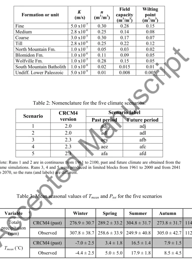
The five “delta change” climate scenarios for the future period were used to drive the infiltration model HELP. Adj represents the driest scenario, while adl is the wettest with, respectively, 1146 and 1251 mm/y total precipitation, corresponding to increases of 2% and 12% compared to the baseline scenario (observations). The warmest scenarios are adl and aez-afc, with a mean annual temperature of 9.93˚C, while adj and aey-afb are the coolest, with mean temperatures of 9.50 and 9.53˚C. Compared to observations from the 1971-2000 period, these temperatures represent increases of 3.16˚C and 2.73˚C (or 2.76˚C for aey-afb), respectively. In all future scenarios, Tmean is always higher than observations: by 3.0˚C on average and by 2.1 to 5.8˚C on a monthly basis. Total precipitation is generally higher in the future for the months of November to April (with the largest increase, of 51%, obtained in December for scenario adl), but relatively unchanged from May to October (except for the adl scenario, which maintains a steadier variation throughout the year; see Figure 11 below). As an example of the results obtained by applying the delta change method, Figure 8 shows the monthly values for the afa-afd future period compared to the observation record for the 1971-2000 period.
3.3 Current-day conditions simulated with HELP
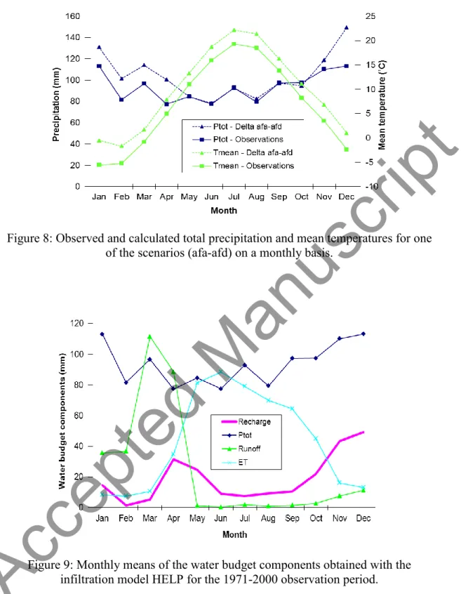
The model HELP was calibrated and run with observations from the 1971-2000 period in a previous study (Rivard et al., 2013). The results for the main hydrological budget components on a monthly basis are shown in Figure 9. Evapotranspiration (ET) constitutes the most important component with 46% of annual total precipitation, while surface and subsurface runoff total 34% (27% and 7% respectively). Based on the runoff curve, spring snowmelt begins in March and continues into April, which is
Accepted Manuscript
slightly earlier than elsewhere in eastern Canada, owing to the micro-climate of the Annapolis Valley. Two main recharge periods can be observed: in the spring (April and May) and in the autumn/winter. Interestingly, the second recharge period appears to be as important as the spring one, due to high precipitation and low evapotranspiration, and to the fact that the soil remains unfrozen for the most part. The mild maritime conditions even allow for recharge in January. For more details see Rivard et al. (2013).
Mean actual evapotranspiration was found to be 519±55mm/y, surface runoff 300±84mm/y, subsurface runoff (hypodermic flow) 73±21mm/y, and recharge 229±48mm/y over the entire study area and 30-year observation period (Table 4). Because the sedimentary formations are composed of different units that are lenticular in nature, forming aquifer/aquitard sequences that are not well known at the regional scale, the recharge component was subsequently corrected to 165mm/y in consideration of the percentage of surface area estimated to be underlain by confined aquifer conditions, based on groundwater level data from different sources (Rivard et al., 2013). The difference (230-165) was attributed to surface/subsurface runoff, which was consequently increased to 365 mm/y. The high values of surface runoff can be attributed to spring snowmelt and the geology and topography of the study area (for instance the steep and low permeability North Mountain cuesta contains many natural springs), and are consistent with other modeling studies in the region (e.g., Gauthier et al., 2009). The results of the climate change scenario simulations run with HELP are presented in the next section as increases or decreases relative to a baseline scenario (reference period). Because only relative numbers are used, this correction to the recharge and surface runoff components has not been taken into account.
4. RESULTS
4.1 Climate change scenarios
Table 4 presents the annual values for groundwater recharge and other water budget components obtained with the HELP model for the five climate scenarios, as well as the total precipitation and mean temperature inputs to the model and the water budget components for the baseline case. All future climate scenarios provide more recharge
Accepted Manuscript
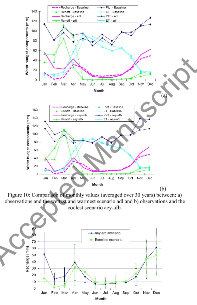
to the aquifer annually than it currently receives (from 14 to 45% higher). As expected, the wettest scenario (adl) results in the largest annual recharge, and the driest (adj) in the smallest. These represent the most contrasted scenarios, at least for the recharge component, with, respectively, 333±83 and 262±55 mm/y over 30 years. Annual ET values for the future period vary little from one scenario to another, from 547±58 to 566±59 mm/y, corresponding to an increase of only 5 to 9%. This is mainly attributed to small temperature variations between scenarios (Tmean from 9.50 to 9.93˚C). The baseline ET value is only 9% lower than the highest value, despite the annual temperature increase of almost 3˚C. The largest temperature increase, however, occurs in the winter, when ET is low. Annual runoff decreases from 9 to 23% (231±91 to 273±92 mm/y) compared to the baseline, likely because more recharge occurs during the winter (for example see Figure 10) since there are more frost-free days and thus less precipitation falls as snow (from 24.5% for observations to 11.8% on average for the 5 future scenarios). Lateral drainage (hypodermic flow) increases from 21 to 63%, mainly due to the increase in Ptot and the fact that more infiltration takes place. This increase seems large, but in absolute terms lateral drainage is the smallest component of the water budget for the study area.
To better understand the system behavior, monthly values for the five climate scenarios have been examined. Figure 10 presents a comparison between the baseline scenario (i.e., using observations) and two of the future scenarios (adl and aey-afb). All five scenarios show similar behavior, except for the first months of the calendar year. For instance runoff, which is generally very similar for all future scenarios, is quite high in February and March for scenario aey-afb (Figure 10b) due to lower infiltration/recharge for the first two months of the year resulting from much cooler temperatures. The runoff peaks for all future scenarios decrease more sharply in April compared to the baseline case, likely because of less snow accumulation during the winter and higher spring temperatures that favor earlier snowmelt and soil thawing. Runoff is practically nil from May to September for all scenarios including the baseline due to high temperatures (mean daily temperatures vary from 13.3 to 22.6˚C) and thus high evapotranspiration, and to low rainfall (minimum levels for the year) and hence low levels of soil saturation . Future runoff values are higher compared to past conditions in the winter because increased Ptot and milder temperatures result in more precipitation falling as rain. The ET curves are relatively similar for all five
Accepted Manuscript
future scenarios, except from May to September when fairly large variations are obtained mostly due to variations in Ptot. Compared to the baseline, future ET is slightly higher during the winter, and markedly higher during the spring, especially in April, while it is lower during the summer despite temperatures that are about 3˚C higher. This is mainly due to the decreased Ptot for this season (see section 4.2).
The simulated future recharge is larger, on average, from November to April, with the first three months (January to March) being much larger, generally with an increase of more than 200%. The largest differences are observed in February. Recharge from May to October, corresponding to the growing season, is reduced in the future, from 4 to 33% depending on the month and climate scenario, with a mean decrease of 17% for these six months and the five scenarios. Such a decline in recharge during the growing season can be of concern for this agricultural region. For both current and future periods, the model simulates a winter recharge that is even more pronounced than in the spring, due to the Valley’s mild climate. This feature is amplified in the future, due to the temperature increase that augments the fraction of precipitation that falls as rain over snow and thereby also the infiltration and recharge amount. Monthly variations for recharge are quite large over the 30-year simulations (see Figure 11), with coefficients of variation (CV = standard error σ / mean μ) varying from 41% to 240% for the baseline scenario and from 45% to 144% for the five climate change scenarios. For a given month, CV values for observations and the five scenarios are of the same order of magnitude, except for February, due to the very low recharge value of the baseline scenario. The largest variations in magnitude are associated with the largest recharge values, i.e., to the months November, December, January (only for the future period) and April, as illustrated in Figure 11.
4.2 Sensitivity analysis
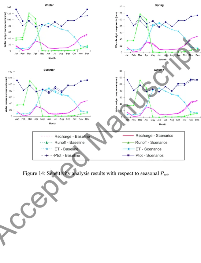
A sensitivity analysis was performed with respect to Tmean and Ptot to investigate seasonal effects on water budget partitioning. The mean variation of each of these variables was used in turn (keeping the other variable fixed) for a given season and for the five scenarios. Table 5 presents the seasonal variations used to perturb the baseline scenario and Figures 12 and 14 present the sensitivity results with respect to temperature and precipitation, respectively.
Accepted Manuscript
The analysis for Tmean shows that the increase in temperature for the summer and autumn seasons has practically no influence on the water budget results, including, somewhat surprisingly, ET summer values. This is probably due to the vegetation properties in the HELP model (e.g., root depth and LAI) that have to be fixed by the modeler and that were not modified as a function of temperature due to absence of data, and to the very low runoff at this time of year. The increase in temperature for the winter and spring seasons, on the other hand, has a considerable influence on the runoff and recharge curves, due to the reduced snow/rain ratio and increased ET (and thus less snow accumulation), and a longer frost-free period allowing more infiltration. Annual changes are illustrated in Figure 13 for the four sensitivity scenarios using seasonal temperature changes and are compared to the simulation run with observations (baseline scenario).
The winter temperature increase has a marked impact on the winter and early spring recharge and runoff values: runoff is considerably reduced in March and April and recharge increases from December to March, being especially high in January. This is by far the sensitivity scenario for which water budget components are most affected by temperature changes, with an increase of 18% (41 mm) in annual recharge and a decrease of 23% (70 mm) in annual runoff. The spring temperature increase causes a shift in the recharge curve: there is a considerable increase in runoff for March (earlier snowmelt) and recharge is almost doubled compared to the baseline scenario. A large decrease in runoff is then observed for April that is accompanied by a large increase in both ET and recharge since water can infiltrate without snow cover. Annual runoff is noticeably affected, with a decrease of 9%. All other water budget components (not mentioned above) have a difference with the baseline scenario of less than 4%.
Compared to temperature effects, the impact of precipitation on the water budget components (Figure 14) is more direct since water is added to or removed from the system, but more limited both in magnitude (amount of change in the component) and in time (duration of the change beyond the perturbed season), at least for the range of seasonal decrease/increase examined here (i.e. from 94% to 118% as reported in Table 5). In general, an increase in precipitation results in higher runoff
Accepted Manuscript
and recharge for the perturbed season (winter, spring, and autumn scenarios) and vice versa (summer scenario). As expected, winter is the only season for which precipitation has an impact on another season (spring): the increase in Ptot during the winter produces an increase in runoff over both the winter and spring seasons. The increase in recharge, however, is limited to the winter season. All ET curves are very similar to that of the baseline scenario, except for the summer scenario where the projected decrease in precipitation is accompanied by a decrease in ET. Recharge is little affected by the seasonal sensitivity analysis of precipitation: differences with the baseline scenario range from -2 to +4%. The only notable differences with respect to the baseline scenario are associated with runoff for the winter and spring scenarios (increases of 7 and 15%, respectively).
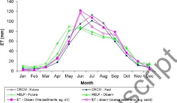
A sensitivity analysis was also performed on secondary variables such as seasonal humidity and wind speed because the ET curve estimated by HELP using observations appears to be quite low during the summer, in comparison to values obtained from the CRCM4 model and Environment Canada. The ET calculation for the climate model is based on the Penman-Monteith equation in both the global and regional models through their soil-vegetation module. Environment Canada uses a weekly water budget based on an improvement of the Phillips (1976) method, with daily temperature and precipitation as inputs. Actual ET is estimated using potential ET calculated with the Thornthwaite method together with water holding capacity and soil storage to assess antecedent moisture conditions. Since wind speed monthly values were 15 ± 5 km/h, the sensitivy analysis was carried out using values of 10 and 20 km/h. Humidity was varied between 60 and 80%, since the seasonal values were 77, 71, 74, and 77%. Figure 15 compares monthly values obtained with 1) HELP for the baseline scenario and for the average of the five future scenarios; 2) observations for fine and coarse soils; and 3) CRCM results for past and future periods averaged over the five scenarios. The fine soil shown in Figure 15 has a larger water-retention capacity than the coarse soil, so that water close to the surface is more available for evapotranspiration. Note that the HELP model calculates potential ET with the Penman equation (see section 3.1), with actual ET then estimated from available water storage at or near the surface. Soil humidity is probably low in the summer for the HELP simulation runs: recharge and especially runoff values are small and large quantities of water are taken by vegetation as plants grow. The sensitivity analysis
Accepted Manuscript
showed that HELP is not very sensitive to humidity and wind speed and this may account for the differences with the CRCM/Environment Canada results.
It can also be observed in Figure 15 that the CRCM4 model generates higher future ET values throughout the year (following the temperature pattern) compared to the past period, especially from April to July with increases from 9 to 15 mm/month (representing an increase of 9 or 10% for the months of May to July and 86% for April). On the other hand, future ET values obtained with HELP decrease slightly during the summer compared to values of the baseline scenario due to a decrease in Ptot. This may be due in large part to the fact that the HELP model does not fully consider vegetation processes. It does not take into account stomatal conductance (which would be reduced in response to a CO2 increase), and parameters such as leaf area index, root depth, and growing season duration must be estimated by the user. Appropriate data for these parameters are not always readily available, especially in a changing climate. The differences between CRCM4 values and observations during the summer may also be due to the fact that precipitation for this period is over-estimated (22% on average compared to observations) by CRCM4, thereby necessitating the application of a transfer scheme such as the delta change method.
5. DISCUSSION AND CONCLUSION
Although there is broad consensus in the scientific community that surface temperatures will increase over the next decades, the regional and local impacts of climatic changes on the various components of the hydrological cycle are still very uncertain and need more research. The impact of climate on recharge is not linear and it is therefore not clear what will be the impact of climate change on aquifer recharge. The amount of precipitation and its state (snow or rain) will be modified and temperatures will increase, resulting in altered magnitudes and patterns of runoff, evapotranspiration, and ultimately recharge. The potential effects of climate change on aquifer recharge have been studied with various models in different regions across Canada and for various periods, producing a wide range of results (e.g., Jyrkama and Sykes, 2007; Scibek and Allen, 2006; Chen et al., 2004).
Accepted Manuscript
The area selected for this study is the Annapolis Valley, located in Nova Scotia (eastern Canada). Total annual precipitation in the region is currently on the order of 1120 mm and predicted climate change scenarios generally agree on a small increase in the next decades (8% on average for the five scenarios used in this study). Economic development in this region is based essentially on agriculture and its derivatives, and most residents and municipalities use groundwater for water supply.
A slight decrease in annual recharge in the Maritime region of eastern Canada was suggested in Rivard et al. (2009) in their Canada-wide study, despite a general increase in total precipitation, based on an analysis of statistical trends in historical records of streamflow (from which baseflow was estimated) and groundwater levels. In the current study, recharge projections and a sensitivity analysis were conducted using a one-dimensional (quasi 2D) water budget model and climate scenarios generated from a combination of historical observations and climate model projections. The projections were produced using a regional climate model and five members for a given greenhouse gas emissions scenario. The simulations yield an annual increase in recharge of 14 to 45% over 30 years. The two studies, executed at different scales and based on different methodological approaches, are nonetheless in agreement in showing that recharge trends vary on a seasonal basis. For instance, the simulation-based approach showed a marked decrease in the summer for the future, while winter values considerably increased. Statistical trends also showed a clear summer decrease and a winter increase in many regions (although the latter was not specifically observed in the Maritimes with the few available stations).
Differences between the two approaches (namely in annual recharge projections) may be attributed in large part to uncertainties in the future climate and in the numerical models. Climate models are of course approximations (although they are very complex) that can only imperfectly represent major processes in the atmospheric-ocean-earth system, while GHG emissions scenarios are extrapolations of actual human behavior, expected technological advances, and demographic changes. Hydrological models likewise use many hypotheses and simplifications to represent real systems. On the other hand, statistical trends use historical (and thus real) data. However, what has occurred in the last 30-40 years may not be representative of the future climate. In addition, geological conditions in the
Accepted Manuscript
monitoring well areas, and therefore groundwater age as well as recharge and discharge zones, were not well known. Therefore, some of the wells may only reflect conditions of 50 or even 5000 years ago. Although imperfect, climate models, in combination with hydrological models, represent a valuable tool for gaining insight into the relationship between climatic conditions and hydrological responses and for studying potential changes in the various water budget components for a given region. The net recharge estimates obtained by Rivard et al. (2013) using a combination of five assessment approaches ranged from 80 to 175 mm/y for the entire Annapolis Valley (2100 km2). These values include a correction factor for some of the approaches, including the HELP model (as mentioned in section 3.3), which do not consider hydrogeological (confined versus unconfined) conditions and thus do not mask out areas where recharge is not possible. This range of estimates is fairly large, owing to the diversity of methods used and reflecting the difficulty of obtaining reliable and accurate values for this key state variable. The 01DC005 station watershed, comprising a quarter of the Valley area, was used for the HELP model, as it was considered representative of the whole Valley in its physiographic, geologic, hydroclimatic, and land use conditions. The range of increase in recharge in response to five climate change scenarios obtained in this study is 30 to 100 mm/y (see Table 4). This interval is smaller than the range obtained in the regional study, as could be expected given the larger scale and the diversity of approaches used in the regional study and the fact that the scenarios are all derived from a single climate model in the current study. It is clear that the combination of different climate change scenarios, hydrogeological prediction models, and recharge estimation techniques will lead to a very broad range of possible impacts that need to be considered in developing future water management plans.
Simulation runs in the current study showed that recharge in the winter will increase due to rising temperatures, while summer recharge will decrease in response mainly to a drop in precipitation. Climate changes are also expected to result in an increase in ET in the winter and, even more markedly, in the spring. The autumn season appears quite stable. These results are in general agreement with other modeling studies such as those of Eckhardt and Ulbrich (2003), Jyrkama and Sykes (2007), and Toews and Allen (2009). Other considerable changes in the spring, such
Accepted Manuscript
as earlier and reduced spring runoff, have also been produced from the simulations, consistent with the results of Burn and Hag Elnur (2002) and Zhang et al. (2001) based on historical records.
This study has stressed the importance of assessing climate change impacts not only on annual water budget distributions but also on monthly and seasonal patterns. Simulation results suggest that the main increase in annual recharge comes from the fact that increased ET does not compensate for the much larger winter infiltration. In addition, some of the findings of this study, namely the 17% mean decrease in recharge during the growing season and the increased evapotranspiration in the spring, may have important implications for water management practices in the region, and in a broader sense on the agricultural economy of the Annapolis Valley. A decrease in recharge during the growing season may eventually lower water levels during this crucial period, leading to potential major impacts on groundwater supply and infrastructure. Some shallow wells in the Valley may need to be drilled deeper and dug wells may have to be abandoned and replaced by drilled wells due to the occurrence of dry wells during the summer. Indeed, the five equiprobable future scenarios provide a global mean that is above the current recharge rate of 230 mm/y, but some individual years from these scenarios show recharge values below this value, especially in the adj scenario (8/30 years, i.e. 27%). Moreover, altered irrigation practices in response to climate change (increased ET, longer growing season) could translate into additional pressure on groundwater resources, a feedback that was not taken into account in the present study. Modeling studies, including future ones that would improve on this and previous studies (by considering feedbacks, additional processes, updated IPCC scenarios, uncertainty estimation, etc.) may play an important role in planning for future potential water stress.
Acknowledgements This study was funded through the Groundwater Program of the Geological Survey of Canada. The project also received support from Nova Scotia Environment (NSE), Agriculture and Agri-Food Canada (AAFC), and the Clean Annapolis River Project (CARP). The authors would like to thank Dr. Richard Fernandes for fruitful discussions, Dr. Uta Gabriel for her careful reading of an early manuscript, and the reviewers for their detailed and helpful comments. This paper is GSC contribution No 15549.
Accepted Manuscript
References
Anandhi, A., Frei, A., Pierson, D. C., Schneiderman, E. M., Zion, M. S., Lounsbury, D., and Matonse A. H. 2011. Examination of change factor methodologies for climate change impact assessment. Water Resources Research, 47, W03501, doi:10.1029/2010WR009104.
Arnell, N.W., Liu, C., Compagnucci, R., da Cunha, L., Hanaki, K., Howe, C., Mailu, G., Shiklomanov, I., and Stakhiv, E. 2001. Hydrology and water resources. Climate Change 2001: Impacts, Adaptation and Vulnerability. Contributions of Working Group II to the Third Assessment Report of the Intergovernmental Panel on Climate Change, J.J. McCarthy, O.F. Canziani, N.A. Leary, D.J. Dokken, and K.S. White, Eds., Cambridge University Press, Cambridge, 191-234.
Burn, D.H. and Hag Elnur, M.H. 2002. Detection of hydrologic trends and variability. Journal of Hydrology, 255, 107-122.
Caya, D. and R. Laprise. 1999. A semi-implicit semi-Lagrangian regional climate model: The Canadian RCM, Monthly Weather Review, 127, 341-362.
Chen, Z., Grasby, S.E., and Osadetz, K.G. 2004. Relation between climate variability and groundwater levels in the upper carbonate aquifer, southern Manitoba, Canada, Journal of Hydrology, 290, 44-62.
de Elía, R. and Côté, H. 2010. Climate and climate change sensitivity to model configuration in the Canadian RCM over North America. Meteorol. Z., 19(4), 325-339. doi: 10.1127/0941-2948/2010/0469.
Eckhardt, K. and Ulbrich, U. 2003. Potential impacts of climate change on groundwater recharge and streamflow in a central European low mountain range, Journal of Hydrology, 284, 244–252.
Accepted Manuscript
Ehret, U., Zehe, E., Wulfmeyer, V., Warrach-Sagi, K., and Liebert, J. 2012. Should we apply bias correction to global and regional climate model data?, Hydrology and Earth System Sciences Discussion, 9, 5355-5387, doi:10.5194/hessd-9-5355-2012. Gauthier, M.-J., Camporese, M., Rivard, C., Paniconi, C., and Larocque, M. 2009. A modeling study of heterogeneity and surface water–groundwater interactions in the Thomas Brook catchment, Annapolis Valley (Nova Scotia, Canada), Hydrology and Earth System Sciences, 13, 1583-1596.
Giorgi, F. and Marinucci, M. R. 1996. An investigation of the sensitivity of simulated precipitation to the model resolution and its implications for climate studies. Monthly Weather Review, 124, 148-166.
Goderniaux, P., Brouyere, S., Blenkinsop, S., Burton, A., Fowler, H. J., Orban, P., and Dassargues, A. 2011. Modeling climate change impacts on groundwater resources using transient stochastic climate scenarios, Water Resources Research, 47, W12516, doi:10.1029/2010WR010082.
Guay, C., Nastev, M., Paniconi, C., and Sulis, M. 2013. Comparison of two modeling approaches for groundwater–surface water interactions, Hydrological Processes, 27, 2258-2270, doi:10.1002/hyp.9323.
Hagemann, S., Chen, C., Haerter, J. O., Heinke, J., Gerten, D., and Piani, C. 2011. Impact of a statistical bias correction on the projected hydrological changes obtained from three GCMs and two hydrology models, Journal of Hydrometeorology, 12(4), 556-578, doi:10.1175/2011jhm1336.1.
Hamblin, T. 2004. Regional geology of the Triassic/Jurassic Fundy Group of Annapolis Valley, GSC Open File 4678.
IPCC. 2007. Climate Change 2007: The Physical Science Basis - Summary for Policymakers - Contribution of Working Group I to the Fourth Assessment Report of the Intergovernmental Panel for Climate Change. Geneva, 18 p.
http://www.risknat.org/projets/climchalp_wp5/pages/rapports/ipcc_sp_2007.html
Accepted Manuscript
Jackson, C. R., Meister, R., and Prudhomme, C. 2011. Modelling the effects of climate change and its uncertainty on UK Chalk groundwater resources from an ensemble of global climate model projections, Journal of Hydrology, 399, 12–28. Jyrkama, M.I. and Sykes, J.F. 2007. The impact of climate change on spatially varying groundwater recharge in the Grand River watershed (Ontario), Journal of Hydrology, 338, 237-250.
McCallum, J. L., Crosbie, R. S., Walker, G. R., and Dawes, W. R. 2010. Impacts of climate change on groundwater in Australia: a sensitivity analysis of recharge, Hydrogeology Journal, 18, 1625-1638.
Monfet, J. 1979. Évaluation du coefficient de ruissellement à l’aide de la méthode SCS modifiée [Assessment of the runoff coefficient using a modified SCS method]. Service de l’hydrométrie, Ministère de l’Environnement du Québec, Publication HP-51.
Nakicenovic, N., Alcamo, J., Davis, G., de Vries, B., Fenhann, J., Gaffin, S., Gregory, K., Grübler, A., Jung, T.Y., Kram, T., La Rovere, E.L., Michaelis, L., Mori, S., Morita, T., Pepper, W., Pitcher, H., Price, L., Riahi, K., Roehrl, A., Rogner, H.-H., Sankovski, A., Schlesinger, M., Shukla, P., Smith, S., Swart, R., van Rooijen, S., Victor, N., Dadi Z. 2000. IPCC Special Report on Emissions Scenarios, Cambridge University Press, Cambridge, United Kingdom and New York, NY, USA. 599pp. http://www.grida.no/climate/ipcc/emission/index.htm
Penman, H. L. 1963. Vegetation and hydrology, Technical comments No. 53, Commonwealth Bureau of Soils, Harpenden, England.
Phillips, D.W. 1976. Monthly water balance tabulations for climatological stations in Canada. D.S. #4-76, Atmospheric Environment Service, Environment Canada, Downsview, Ontario.
Accepted Manuscript
Raupach, M.R., Marland, G., Clals, P., Le Quéré, C., Canadell, J.G., Klepper, G. and Field, C.B. 2007. Global and regional drivers of accelerating CO2 emissions, Proc.Nat.Aca.Sci., 11104, 10288-10293.
Rivard, C., Paradis, D., Paradis, S.J., Bolduc, A., Morin, R.H., Liao, S., Pullan, S., Gauthier, M.-J., Trépanier, S., Blackmore, A., Spooner, I., Deblonde, C., Boivin, R., Fernandes, R.A., Castonguay, S., Hamblin, T., Michaud, Y., Drage, J., and Paniconi, C. 2012. Canadian Groundwater Inventory: Regional Hydrogeological Characterization of the Annapolis Valley Aquifers. GSC Bulletin no 598.
Rivard, C., Lefebvre, R., and Paradis, D. 2013. Regional recharge estimation using multiple methods: an application in the Annapolis Valley, Nova Scotia (Canada), Environmental Earth Sciences,DOI 10.1007/s12665-013-2545-2.
Rivard, C., Vigneault, H., Piggott, A.R., Larocque, M., and Anctil, F. 2009. Groundwater recharge trends in Canada, Canadian Journal of Earth Sciences, 46, 841-854.
Schroeder, P.R., Lloyd, C.M., and Zappi, P.A. 1994. The hydrologic evaluation of landfill performance (HELP) model, User’s guide for version 3, Interagency Agreement No. DW21931425, 233 p.
Scibek, J. and Allen, D. M. 2006. Modeled impacts of predicted climate change on recharge and groundwater levels, Water Resources Research, 41, W11405, 18 p. Scinocca, J. F., N. A. McFarlane, M. Lazare, J. Li, and Plummer, D. 2008. Technical Note: The CCCma third generation AGCM and its extension into the middle atmosphere. Atmos. Chem. Phys, 8, 7055-7074.
Stoll, S., Hendricks Franssen, H. J., Butts, M., and Kinzelbach, W. 2011. Analysis of the impact of climate change on groundwater related hydrological fluxes: a
multi-Accepted Manuscript
model approach including different downscaling methods, Hydrology and Earth System Sciences, 15(1), 21–38.
Sulis, M., Paniconi, C., Rivard, C., Harvey, R., and Chaumont, D. 2011. Assessment of climate change impacts at the catchment scale with a detailed hydrological model of surface-subsurface interactions and comparison with a land surface model, Water Resources Research, 47, W01513, doi:10.1029/2010WR009167.
Sulis, M., Paniconi, C., Marrocu, M., Huard, D., and Chaumont, D. 2012. Hydrologic response to multimodel climate output using a physically-based model of groundwater/surface water interactions, Water Resources Research, 48, W12510, doi:10.1029/2012WR012304.
Todd, D.K. 1980. Groundwater Hydrogeology. Second edition, John Wiley and Sons, New York.
Toews, M.W. and Allen, D.M. 2009. Evaluating different GCMs for predicting spatial recharge in an irrigated arid region, Journal of Hydrology, 374(3-4), 265-281.
van Roosmalen, L., Sonnenborg, T.O., and Jensen, K.H. 2009. The impact of climate and land use change on the hydrology of a large-scale agricultural catchment. Water Resour. Res., 45,W00A15, doi:10.1029/2007WR006760.
Zhang, X., Harvey, K.D., Hogg, W.D., and Yuzyk, T.R. 2001. Trends in Canadian streamflow, Water Resources Research, 37(4), 987-998.
Accepted Manuscript
Table 1: Subsurface parameter values used in HELP. Formation or unit (m/s) K (m3n /m3) Field capacity (m3/m3) Wilting point (m3/m3) Fine 5.0 x10⁻⁷ 0.30 0.28 0.15 Medium 2.8 x10⁻⁶ 0.25 0.14 0.08 Coarse 3.0 x10⁻⁵ 0.30 0.17 0.07 Till 2.8 x10⁻⁶ 0.25 0.22 0.12 North Mountain Fm. 1.0 x10⁻⁷ 0.05 0.03 0.02 Blomidon Fm. 1.0 x10⁻⁶ 0.11 0.09 0.05 Wolfville Fm. 1.0 x10⁻⁵ 0.28 0.15 0.05
South Mountain Batholith 1.0 x10⁻⁸ 0.02 0.015 0.01
Undiff. Lower Paleozoic 5.0 x10⁻⁹ 0.01 0.008 0.005
Table 2: Nomenclature for the five climate scenarios.
Scenario CRCM4
version
Scenario label
Past period Future period
1 2.0 adj adj
2 2.0 adl adl
3 2.3 aey afb
4 2.3 aez afc
5 2.3 afa afd
Note: Runs 1 and 2 are in continuous from 1961 to 2100, past and future climate are obtained from the same simulations. Runs 3, 4 and 5 were produced in limited blocks from 1961 to 2000 and from 2041 to 2070, so the runs (and labels) are different.
Table 3: Mean seasonal values of Tmean and Ptot for the five scenarios
Variable Winter Spring Summer Autumn Annual
Total precipitation (mm) CRCM4 (past) 276.9 ± 30.7 289.2 ± 33.2 304.8 ± 31.7 273.8 ± 31.7 1144.9 ± 107.9 Observed 307.8 ± 38.7 258.6 ± 33.9 249.9 ± 40.8 305.0 ± 42.7 1121.3 ± 130.0 Tmean (˚C) CRCM4 (past) -7.0 ± 2.5 3.4 ± 1.8 16.5 ± 1.4 7.9 ± 1.5 5.2 ± 0.8 Observed -4.4 ± 2.5 5.0 ± 5.0 17.9 ± 1.8 8.5 ± 4.5 6.7 ± 0.7
Accepted Manuscript
Table 4: Annual water budget components for the five climate scenarios (2041-2070) and for the baseline case (1971-2000). The light grey cells show standard errors. The darker grey cells highlight the mean total precipitation and recharge for the driest and
wettest scenarios.
Scenario standard Mean / error
Ptot Tmean Runoff ET Lateral Recharge
(mm) (˚C) (mm) (mm) drainage (mm) (mm) Baseline
μ
1121.3 6.77 300.3 519.2 72.3 229.5 σ 129.9 0.75 84.4 54.7 20.6 48.0 adjμ
1145.6 9.50 245.5 550.4 87.5 262.2σ
135.3 0.74 77.8 63.2 22.6 55.4 adlμ
1250.7 9.93 250.9 546.9 119.5 333.4σ
148.4 0.74 105.4 57.9 33.3 82.8 aey-afbμ
1226.2 9.53 273.0 559.5 100.5 293.2σ
140.6 9.74 92.0 59.6 23.3 58.9 aez-afcμ
1177.6 9.93 231.2 553.8 100.7 291.9σ
135.8 0.74 90.6 58.5 29.1 70.8 afa-afdμ
1244.4 9.84 257.5 565.6 109.0 312.3σ
143.6 0.74 97.3 58.8 26.4 67.2Table 5: Seasonal variations resulting from the five scenarios averaged over 30 years and used in the sensitivity analysis.
Season Tmean (˚C) Ptot (%)
Winter +3.76 117.8%
Spring +2.92 113.4%
Summer +2.82 94.1%
Autumn +2.56 104.3%
Accepted Manuscript
Figures
Fig. 1 Location of the study area (watershed 01DC005, 546 km<sup>2<sup>).
Fig. 2 Simplified bedrock geology map (from Rivard et al., 2012).
Accepted Manuscript
Fig. 3 Regional scale conceptual model (adapted from Rivard et al., 2009).
Fig. 4 Percentages of the four CRCM tiles covering the study area.
Accepted Manuscript
(a)
(b) Fig. 5 Comparison between observations (from the Greenwood station) and simulated data for the five regional climate simulations for a) annual total precipitation and b) annual minimum temperature. Box plots include maximum, minimum, median, and 25 and 75th percentile values.
Accepted Manuscript
Figure 6: Monthly values of mean temperature (Tmean) and total precipitation (Ptot) for the afa simulation and observations from the Greenwood station.
Accepted Manuscript
(a)
(b) Figure 7: Differences between future and past conditions for the five climate scenarios
used in this study for a) monthly mean total precipitation and b) monthly mean temperature.
Accepted Manuscript
Figure 8: Observed and calculated total precipitation and mean temperatures for one
of the scenarios (afa-afd) on a monthly basis.
Figure 9: Monthly means of the water budget components obtained with the infiltration model HELP for the 1971-2000 observation period.
Accepted Manuscript
(a)
(b)
Figure 10: Comparison of monthly values (averaged over 30 years) between: a) observations and the wettest and warmest scenario adl and b) observations and the
coolest scenario aey-afb.
Figure 11: Temporal variations in the recharge component over the 30-year period.
Accepted Manuscript
Recharge - Baseline Ptot - Baseline Runoff - Baseline ET - Baseline Recharge - Scenarios Runoff - Scenarios ET - Scenarios
Mean temperature - Scenarios Mean temperature - Baseline
Figure 12: Sensitivity analysis results with respect to seasonal Tmean.
Figure 13: Water budget components for the four sensitivity scenarios using mean seasonal temperatures. Total precipitation is constant (Ptot=1121 mm/y).
Accepted Manuscript
Ptot - Scenarios Recharge - Baseline Ptot - Baseline Runoff - Baseline ET - Baseline Recharge - Scenarios Runoff - Scenarios ET - Scenarios
Figure 14: Sensitivity analysis results with respect to seasonal Ptot.
Accepted Manuscript
Figure 15: Monthly ET values averaged over 30 years for the past and future periods (averaged over the five scenarios) as simulated by the HELP and CRCM models, as
well as observations for two soil types obtained from Environment Canada.