The
influence of model structure on groundwater recharge rates
in
climate-change impact studies
Christian Moeck1,2 & Philip Brunner1 & Daniel Hunkeler1
Abstract Numerous modeling approaches are available to provide insight into the relationship between climate change and groundwater recharge. However, several aspects of how hydrological model choice and structure affect recharge pre-dictions have not been fully explored, unlike the well-established variability of climate model chains—combination of global climate models (GCM) and regional climate models (RCM). Furthermore, the influence on predictions related to subsoil parameterization and the variability of observation da-ta employed during calibration remain unclear. This paper compares and quantifies these different sources of uncertainty in a systematic way. The described numerical experiment is based on a heterogeneous two-dimensional reference model. Four simpler models were calibrated against the output of the reference model, and recharge predictions of both reference and simpler models were compared to evaluate the effect of model structure on climate-change impact studies. The results highlight that model simplification leads to different recharge rates under climate change, especially under extreme condi-tions, although the different models performed similarly under historical climate conditions. Extreme weather conditions lead to model bias in the predictions and therefore must be consid-ered. Consequently, the chosen calibration strategy is
important and, if possible, the calibration data set should clude climatic extremes in order to minimise model bias in-troduced by the calibration. The results strongly suggest that ensembles of climate projections should be coupled with en-sembles of hydrogeological models to produce credible pre-dictions of future recharge and with the associated uncertainties.
Keywords Groundwater recharge . Climate change . Model complexity . Uncertainty
Introduction
Evaluating the effect of climate change on water resources is essential for their sustainable management. Therefore, numer-ous climate impact studies have been carried out to provide insight into the relationship between climate change and water resources (e.g. Aeschbach-Hertig and Gleeson 2012; Goderniaux et al. 2009; Scibek and Allen 2006b; Green et al. 2011; Newcomer et al.2014; Pulido-Velazquez et al. 2015; Rossman et al. 2014; Shamir et al. 2015; Toews and Allen2009; Woldeamlak et al.2007; Zhang et al.2014among others).
A frequent goal in climate-change impact studies is to quantify groundwater recharge. Groundwater recharge is one of the main drivers of hydrogeological systems (Green et al. 2011; Bakker et al.2013) and a key parameter for sustainable water resource management (Kinzelbach et al. 2003). Currently, a variety of different models are used to estimate recharge in climate-change-impact studies. These models can be grouped into four general categories: (1) simple empirical relationships between precipitation and recharge (e.g. Owor et al.2009; Serrat-Capdevila et al.2007); (2) soil-water-balance models (e.g. HELP model, SMBM, Lumprem, EPIC-GRID * Christian Moeck
1
University of Neuchâtel, Centre for Hydrogeology and Geothermics (CHYN), Neuchâtel, Switzerland
2 Present address: Eawag: Swiss Federal Institute of Aquatic Science
and Technology, Dübendorf, Switzerland
Published in Hydrogeology Journal 24, issue 5, 1171-1184, 2016 which should be used for any reference to this work
soil model; Allen et al.2004; Brouyere et al.2004; Jyrkama and Sykes2007; Mileham et al.2008; Mileham et al.2009; Scibek and Allen2006a; Kurylyk and MacQuarrie2013); (3) soil water balance models embedded within a coupled hydro-logical modeling framework that facilitates more realistic boundary conditions (e.g. FEFLOW and the Mike SHE two-layer water balance model; Stoll et al.2011; van Roosmalen et al.2009; (4) models based on the Richards’ equation (e.g. HydroGepshere, ParFlow and HYDRUS; Ferguson and Maxwell2010; Goderniaux et al.2009,2011; Leterme et al. 2012; Sulis et al.2011,2012).
An important question corresponds to how model choice affects a prediction. Cuthbert and Tindimugaya (2010) dem-onstrated that different groundwater recharge models gave similar long-term historic recharge rates but responded very differently to changes in precipitation intensity. Jiang et al. (2007) used six water balance models and identified differences in future recharge simulations. Hartmann et al. (2012) choose five different lumped models to incorporate model uncertainty for water availability simulations. The dif-ferences in the models had a strong impact on the ensemble-simulated discharge already occurring during the control pe-riod. Bastola et al. (2011) compared the uncertainty from mod-el structure and parameter sets in a climate change study by using four conceptual rainfall-runoff models and two ap-proaches to evaluate parameter uncertainty. They concluded that the role of the hydrological model uncertainty can be remarkably high. In more general terms, Bastola et al. (2011), Crosbie et al. (2011, Holman (2006) and Döll and Fiedler (2008) emphasized that the choice of the hydrogeological model will influence the outcome of climate-change impact studies.
Apart from the chosen model structure, additional sources of uncertainty exist. For example, in its simplest form, a Richards’ equation type model such as HYDRUS can be employed with assumed homogenous subsoil properties. Alternatively, the variability of the hydrologic properties with-in the model domawith-in can be considered by with-increaswith-ing the number of model parameters. As demonstrated in various studies (e.g. Schluter et al.2012; Moeck et al.2015), the degree to which variability of the subsoil is considered can have a profound impact on predictions. In addition to the model parameterization, the chosen calibration strategy is also important. Like for any other model, model parameters employed are typically determined through calibration. The amount of observation data and their variability within the calibration period influence the calibrated parameter values as demonstrated for rainfall-runoff models. For example, whether or not extreme values are present in the observation data set can have a profound impact on the prediction (Coron et al.2012; Merz et al.2011; Seiller et al. 2012; Vaze et al. 2010). Brigode et al. (2013) emphasized that the reliability of models for climate-change impact studies should be increased,
particularly in the development of suitable model structures and calibration strategies that increase their model perfor-mance robustness. Although the effect of the calibration peri-od is known for rainfall-runoff mperi-odels it still remains unclear if groundwater recharge models are also affected.
Only a few studies exist which compare most of the afore-mentioned sources of uncertainty in climate-change impact stud-ies (e.g. Teng et al. 2012; Crosbie et al.2011; Kingston and Taylor2010). Crosbie et al. (2011) compared the uncertainty in recharge prediction among five GCMs, three downscaling methods and four hydrological models. They found that the choice of the GCM gives rise to the largest uncertainty in future recharge estimates followed by the downscaling method. The choice of the hydrological models contributed least to the overall uncertainty. Although Crosbie et al. (2011) indicate gen-eral trends, all predictions are based on homogenous model pa-rameterizations. The effects of the calibration strategy and obser-vation period were not considered and the missing link between the mechanics of the model structure and the recharge under climate change was not established. This however, might be important due to the fact that the models were not always con-sistent in their predictions, even though they perform similarly for the calibration period. Why these discrepancies in model predictions occur still remains unclear; furthermore, little is known about whether the discrepancies in model results are sta-tionary within climate change simulations or whether the results will change by considering different future simulation periods. Consequently, there is a lack of knowledge about the importance of the different types of uncertainty, although the aforementioned studies already indicate a few general trends.
Therefore, these four different sources of uncertainty were considered and compared—namely, the variability related to the climate model chains (GCMs-RCMs combinations), choice of hydrological models, and different parameteriza-tions of models, as well as used observation data employed during model calibration in a systematic way. Predictions of how climate change affects recharge quantity and dynamics are fundamental for developing suitable water-resources-management practices. A solid understanding of how reliable these predictions are is indispensable.
This paper quantifies and compares all these different types of uncertainty using different model performance criteria. More specifically, the following questions are addressed: 1. How the choice of hydrological models influences
predic-tions of recharge is systematically assessed.
2. How different parameterizations of models (e.g. homog-enous vs. heterogeneous) affect predictions of recharge for different climate model chains is assessed.
3. The influence of used observation data employed during model calibration on model performance and predictions is analyzed. Specifically, models are calibrated using ob-servation data covering average climatic conditions only,
and the predictions based on calibrated models under ex-treme weather conditions are compared.
As future recharge rates are unknown, a complex two-dimensional (2D) heterogeneous reference model is used as a proxy for real groundwater systems. This study refers to groundwater systems with minor head fluctuations. The study is based on a lysimeter facility (Zurich Reckenholz) from where the model geometry and dimensions of the 2D hetero-geneous reference model was taken. Furthermore, soil prop-erties, climate forcing functions and predicted changes under climate change were adopted from one lysimeter of the lysim-eter facility. A semi-synthetic approach was chosen due to a variety of farming management practice such as cropping, fallow rotations and tillage at the lysimeter. These actions highly influence all observations required for the model cali-bration; to incorporate all these effects is beyond the scope of this study. Considering changing crop cover associated with irregular and often unknown cropping and harvesting cycles as well as tillage effects would certainly limit a systematic and robust comparison of different model complexities.
Methods and modeling strategy
Simpler models were calibrated against monthly groundwater-recharge time series generated by the reference model, and used as a proxy for real systems. Monthly recharge values were chosen for the calibration. As emphasized by Kresic (2006) monthly values in the model calibration enable one to obtain reliable simulations of seasonal effects, which is very important for long-term predictions on climate change. This choice is widely applied because it allows for relating recharge values to stream discharge (Seneviratne et al.2012). For each of the four aforementioned model categories—simple empir-ical relationships between precipitation and recharge, soil-water balance and semi-mechanistic models, as well as models based on the Richards’ equation—one recharge model was chosen. Calibration was carried out using the automatic parameter estimation software PEST (Doherty2011) for soil and vegetation parameters for each simplified recharge model— Table S1 of the electronic supplementary material (ESM).
Best-estimate model parameters were used to systematically evaluate the model performance under historical and future cli-mate conditions. All recharge models were run for 30 years of daily simulations for four time periods—historic conditions and three future time periods: mid-point 2035 (2021–2050), mid-point 2060 (2045–2074) and mid-mid-point 2085 (2070–2099). In order to estimate uncertainty under future climatic conditions, different GCM-RCM combinations were applied for the three future time periods. Finally, three different calibration periods, containing recharge values from an average year (2010), from a sequence of a wet and a dry year (2002/2003) and from the
2004–2009 period (longer time series with average to slightly dry years), were used to evaluate whether simpler models show less predictive model bias when extreme conditions and longer time series of observation are included in the calibration.
Reference model for recharge estimation
Numerical model
The reference model was constructed using the fully coupled physically based model HydroGeoSphere (HGS; Therrien et al.2010). A control volume finite element approach is used to solve Richards’ equation describing 3D variably saturated subsurface flow. The soil hydraulic model follows the Van Genuchten (1980) formulation. Precipitation is partitioned in-to runoff, infiltration and evapotranspiration (ET), which is calculated following Kristensen and Jensen (1975) and is a function of potential evapotranspiration, soil moisture, evap-oration depth, root depth, and leaf area index (LAI; Brunner and Simmons2012). Infiltration occurs when precipitation exceeds evaporation and interception storage; a more detailed description of the model and all its components can be found in Therrien et al. (2010) and in theESM.
Model setup
The forcing functions, soil properties (hydraulic conductivity range, van Genuchten parameters and porosity) and model di-mensions were based on the Zürich Reckenholz lysimeter. The lysimeter has a surface area of 1 m2and depth of 150 cm. The steel cylinders are filled with undisturbed sandy soil. No over-land flow can occur due to a steel edge surrounding the top of the lysimeter. The measured lysimeter discharge at the bottom of the lysimeter is used to represent groundwater recharge.
Based on the geometry of the lysimeter, a vertical 2D het-erogeneous reference model was created with 150 cm depth in the z-direction, 100 cm in the x-direction and 5 cm discretization horizontally and vertically (Fig.1). This fine discretization was necessary to obtain a numerical solution with reasonable accuracy (Vogel and Ippisch2008).
Soil properties from different depths were used to create hydraulic conductivities based on Rosetta, a program for pedo-transfer functions (Schaap et al.2001). The hydraulic conductivities at different depths were subsequently used to create a variogram for the stochastic field generator to gener-ate the hydraulic conductivity field. Hydraulic conductivity was distributed within the model domain using the program Fieldgen (Doherty 2011), a 2D stochastic field generator, while field generation was undertaken using the Gaussian se-quential simulation principle.
To apply the Richards’ equation, van Genuchten pa-rameters were employed in addition to the generated hy-draulic conductivity. A related challenge to this model
parameterisation is to avoid unrealistic relationships be-tween randomly generated hydraulic conductivities and t h e van Genuchten parameters. Therefore, v a n Genuchten parameters were assigned to each mesh node based on the relationship between hydraulic conductivity and the van Genuchten parameters alpha, beta and resid-ual water content (Carsel and Parrish 1988). The vari-ance associated with this relationship was taken into ac-count. This approach leads to a more realistic represen-tation of natural soils (Fig. S1 of the ESM). In addition, porosity was distributed and adapted from a standard normal Gaussian distribution for the entire soil column and ranged from 0.33 to 0.38, similar to measured values from the lysimeter soil samples; furthermore, in order to represent spatial heterogeneity in a more robust way, 130 stochastic realizations of the soil parameters were carried out. The hydraulic conductivities from different depths were used to create a variogram. Based on these obser-vations, an exponential variogram with a range of 0.5 m and a sill of 0.29 was obtained; however, not only a sill of 0.29 was applied, also different sill values were used to consider moderate and comparatively stronger hetero-geneity in order to cover a wider range of different pos-sible soil structures. A sill of 0.29 was used for 100 realizations and a value of 1 for the remaining 30.
Preliminary consideration of heterogeneity shows, howev-er, that for the considered specific soil type with the associated stochastic realisations, recharge is dominated by precipitation patterns and not by the adopted soil structure. Therefore, a full stochastic analysis was not required, which reduced the com-putational demand considerably; however, in soils with dom-inant macro components or different clay content, it might be different as demonstrated by Kim and Jackson (2012); Lorenz and Delin (2007) and Wohling et al. (2012). Petheram et al.(2002) point out that soil structure becomes more important for higher clay content soils compared to sandy soils. The adopted soil structure in this study can be characterised rather as a sandy soil than a clay or loam.
Model parameters such as root zone and LAI were added to the model to simulate the presence of a constant grass cover. Interception, which involves retention of a certain amount of precipitation, was further included in the model setup. Altogether, 3,014 parameter values describe the 2D heteroge-neous model domain—applied model parameters can be found in Table S2 of the ESM.
A specified flux boundary was applied on the top of the column with daily values for potential ET and precipitation. Although daily values were used for the climatic forcing func-tions, an adaptive time stepping was used for the simulations which ensure that the model is running on sub-daily time steps
Precipitation Actual ET = f (PET, θ, LEAF, Root Depth,
Evaporation Depth)
Fixed head boundary: p = 0 0 cm 150 cm 100 cm 50 cm 100 cm 0 cm 50 cm Recharge
Fig. 1 Soil structure for the heterogeneous synthetic 2D reference model with log saturated hydraulic conductivity distribution from−13 to −7.5 [m s−1] and 150 cm depth in the z-direction, 100 cm in the x-direction and 5-cm discretization horizontally and vertically. A specified flux boundary was applied on the top of the column and a fixed head boundary at the bottom with pressure p = 0. The actual ET rate is a function of potential ET, LEAF, (water content), root depth and evapora-tion depth
when a change in, e.g., saturation occurs. A fixed head boundary was used at the bottom. This chosen boundary, based on the lysimeter setup, might affect the timing of recharge; however, the absolute rates are not affected due to a relatively small ex-tinction depth and evaporation for the considered specific soil with grass cover (Shah et al.2007). No-flow boundary condi-tions were applied to the remaining borders of the soil column. Daily time series of actual precipitation and air temperature were used over a period from 01.01.1982 to 31.12.2011 as model inputs (Fig. S2 of the ESM). Snow accumulation can be neglected due to the temperature pattern at the study area. The time series were measured at the MeteoSwiss weather station in Zurich-Reckenholz, Switzerland, situated at the ly-simeter facility. Potential evapotranspiration was calculated using the Penman-Monteith equation after Allen et al. (2005). The average annual precipitation and potential ET is 900 and 550 mm/year, respectively.
Simplified models for recharge estimation
In this section, the four simplified models are described and a schematic summary of the model structures is given in Fig. S3 of theESM.
& Homogeneous one-dimensional (1D) model (1d1L) As a first simplified model (referred to as 1d1L) a HGS model was used but with a homogeneous model parameter discretization, while maintaining the same conceptualization of the underlying physical processes described for the refer-ence model.
& Lumped parameter bucket model (Lumprem)
The second model was a lumped parameterBbucket^ mod-el named Lumprem, which was successfully used in a modmod-el simplification study by Watson et al. (2013). The model pro-vides a basic representation of the unsaturated zone, including matrix and macropore recharge. Matrix and macropore re-charge are activated after specified delay times. Lumprem calculates the actual evapotranspiration taking soil moisture storage and plant parameters into account. Water is lost from the bucket as unsaturated vertical flow (Fig. S3 of the ESM). The recharge rate depends on the soil moisture quantity in the bucket. The soil moisture quantity also controls the hydraulic conductivity. A decreasing soil moisture store lowers the hy-draulic conductivity, following the concept of the water reten-tion curve.
& Soil-water-balance model (Finch)
In this soil-water-balance model (referred to as Finch) di-rect recharge is calculated using a simple daily water balance.
Recharge occurs when the soil moisture content exceeds the field capacity (von Freyberg et al.2015). Interception and root water uptake was included. Water uptake from plant roots occurs at the given rate as long as there is no water stress. The root zone for the Finch model was divided into four layers (Fig. S3 of the ESM) following the standard approach of Finch (1998). For a more comprehensive description of the model, see Finch (2001), Finch (1998).
& Soil-water-balance model (SWB)
This soil-water-balance model (referred to as SWB) de-pends only on one soil-water storage parameter. Recharge can only occur if the threshold of this parameter is reached. The amount of water surpassing the threshold is equal to re-charge (see Fig. S3 of theESM). Changes in storage result from subtraction of actual evapotranspiration from precipita-tion as well as storage changes from the previous day. A soil function, which depends on the chosen soil storage parameter, reduces the potential for actual evapotranspiration (Richter and Lillich1975).
Model performance evaluation
Different performance criteria are applied in order to quantify the effect of model simplification and different model calibra-tion approaches on recharge prediccalibra-tions under climate change. The application of such multiple performance criteria is gen-erally recommended because a single criterion evaluates only specific aspects of model performance (e.g. Krause et al. 2005). Bennett et al. (2013) mentioned that model perfor-mance criteria which are applicable for one specific model application may not be sufficient for another. The following performance measures were introduced—a modified model-scenario ratio (MSR; Droogers et al.2008), the Nash Sutcliffe model efficiency coefficient (Nash and Sutcliffe 1970) and percent of bias (PBIAS; Gupta et al.1999).
The MSR indicates to what extent the impact of a scenario contributes to predictions compared to model simplification. The MSR has a range from 1 to–∞, where 1 indicates that model simplification does not affect the results and recharge changes are a function of the future forcing functions only. Values less than 0 indicate that model simplification is the dominant factor for changes in recharge rates rather than the scenario. Like the MSR, the NSE also provides values be-tween 1 and–∞, where 1 indicates a perfect match and model simplification does not affect change in future recharge rates. PBIAS provides a measure of over- or underestimation for each scenario. An optimal value is 0 %, while a positive value indicates an underestimation and a negative value an overes-timation of yearly recharge rates. A more detailed description for all applied indicators can be found in theESM.
Climate change scenarios
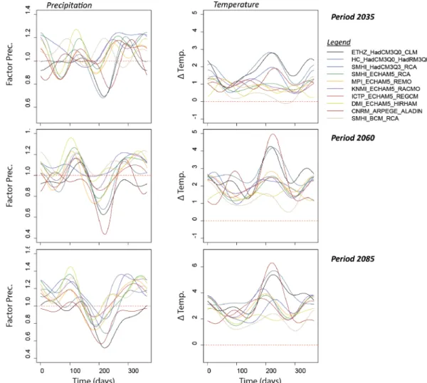
To simulate future climate conditions, a total of ten GCM-RCM model chains (Fig.2and Table S3 of theESM) for the A1B emission scenario were used (CH2011 2011). Thirty time series were created comprising ten model chains for three climate change periods, in order to estimate uncertainty under possible future climatic conditions. The scenarios were de-rived directly from the output of individual GCM-RCM mod-el chains by means of the statistical downscaling technique to the MeteoSwiss monitoring network, with an inverse distance weighting interpolation (Bosshard et al.2011). Bosshard et al. (2011) developed an extension of the simple delta change method that scales observational time series by a climate change signal extracted from climate model output. Thirty-year mean annual cycles of temperature and precipitation were represented by a superposition of harmonics. This method ameliorates the effects of natural variability on artificial fluc-tuations in the annual cycle—more details about the down-scaling method are given in Bosshard et al.2011and CH2011 2011. The obtained model chains provide a daily time series of
delta change factors for precipitation and temperature relative to the reference period 1980–2009 for three time periods: 2035 (2021–2050), 2060 (2045–2074) and 2085 (2070– 2099). Changes in temperature lead directly to changes in ET. In the following analysis, all applied recharge models were run for 30 years of daily simulations for each time period. Note that using only one emission scenario and one downscal-ing method constrained the uncertainty analysis (van Vuuren et al.2011). Using more emission scenarios would certainly increase the uncertainty related to the GCM-RCM combina-tions; however, the used delta change method is still one of the most used approaches in hydrological impact studies (Goderniaux et al.2015); Teutschbein and Seibert2012) and the choice of using one emission scenario is mainly based on several restrictions of the downscaling method to station scale. The restrictions are methodological aspects (some driven model chains can produce an overshooting of climate change signals at some locations; see Bosshard et al. 2011 for details) and reduced data availability on a daily scale (CH2011 2011), as well as length of the simulation period (CH2011 2011).
Fig. 2 Daily climatic change factors (delta-change approach) for each climate model chain for scenario A1B. The left column shows factor changes in daily precipitation, the right column shows mean daily delta temperature changes for the MeteoSwiss weather station in Zurich-Reckenholz
Results
and discussion
In the following section, results of the model calibration of the simpler models against the reference recharge are shown. The best-estimate model parameters were used to systematically evaluate the model performance under historical and future conditions. A comparison between three calibration periods was carried out, in order to evaluate if simpler models show a better model performance if different calibration data sets were applied and, lastly, the relationship between model struc-ture, calibration data set and model performance for climate-change impact studies is addressed.
Calibration under average climatic conditions and validation
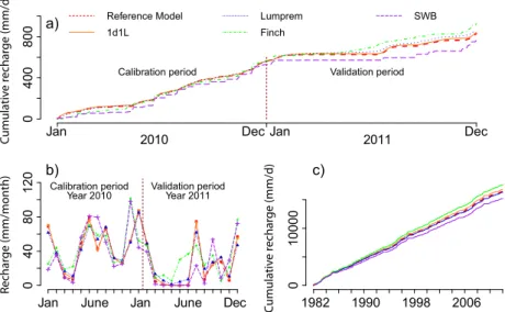
For the calibration period 2010, the simpler calibrated re-charge models reproduced the monthly and cumulative refer-ence recharge surprisingly well, despite considerably different model structures (Fig. 3a,b as well as Table S4 of the ESM).However, sharp rises of recharge after strong precipita-tion events appear for the SWB and Finch model, while the recharge pattern is smoother for the other models. The differ-ent behavior can be directly related to the conceptual model complexity, discussed later. For the validation period 2011–2013, including a year with a long dry spell in spring 2011 (Staudinger et al. 2015), differences in recharge occur for all simpler models, especially for the SWB and Finch model.
Simulating the historical recharge with the reference model for a 30-year period leads to a mean annual value of 543 mm/ year which is very similar to simulated mean annual recharge of 588 mm/year for a study area in northern Switzerland, east of the city of Zurich (Stoll et al. 2011). In addition, similar values are also found in both studies for actual evapotranspiration. Although recharge differences increase for the validation
period between the reference model and the simplified models, the simple models perform quite well for the historical climate conditions (Fig. 3c). This 30-year simulation of historical re-charge shows only small variability among the different models. The SWB model underestimates (−10 %), whereas the Finch model overestimates (+7.5 %) the total recharge rate. Also, the 1d1L and Lumprem models respectively over- and underestimate the predicted value from the reference model, although by less than 2 %.
Model performance for future climate conditions
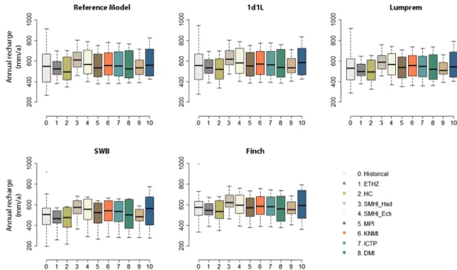
Simulations of recharge for the period 2035 show a large variability in the results (Fig. 4). The mean groundwater re-charge increases by 4.2 % (+22.8 mm) for the 2D reference model considering all 10 climate model chains relative to the historical modelled reference period 1982–2011. However, due to the variability among the different climate model chains, a range of mean change of groundwater recharge be-tween −4.3 % (−23.3 mm) and +14.4 % (+78.1 mm) was simulated. Similar ranges can also be observed for all other groundwater recharge models (Table 1). It is interesting to note that models with increasing simplification tend to under-estimate changes in recharge compared to the more complex reference 2D model. Mean recharge as well as the lower (minimum) and upper bound (maximum) of recharge decrease with increasing model simplification.
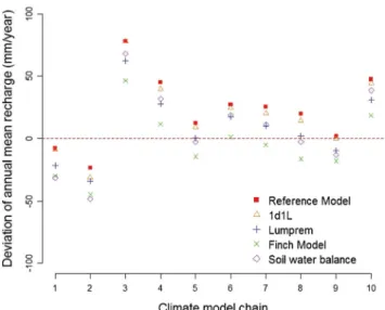
In Fig. 5 deviations of future recharge (2035 period) from the baseline scenario are shown for all models and all climate model chains. The variability is larger among climate model chains than among recharge models. For different climate model chains, the mean deviation of each model spreads over a range of 130 mm/year, while for a given climate model chain, all recharge models fall within a range of 30 mm/year only. The model 1d1L shows recharge values close to
Calibration period Validation period
04 0 0 8 0 0 Jan Dec Reference Model 1d1L Lumprem Finch SWB 04 0 8 0 1 2 0 Jan Calibration period
Year 2010 Validation periodYear 2011
0 10000 1982 1990 1998 2006 C umulativ e r echar ge (mm/d) Rechar ge (mm/month) Jan Dec Jan
June June Cumulativ
e r echar ge (mm/d) Dec 2010 2011 a) b) c)
Fig. 3 a 2D simulated monthly reference recharge (red dashed line) and fitted recharge for 1d1L (orange line), Lumprem (blue line), Finch (green line) and SWB model (purple line) for the 2010 and 2013 period. The 2D reference recharge from the year 2010 was used for the calibration of the simplified models. The recharge values from years 2011– 2013 were used for the validation. b Monthly recharge for the year calibration year 2010 and validation period 2011–2013 and c cumulative daily recharge between 1982–2013
predictions from the reference 2D model. The Finch and SWB models perform differently. Based on the Finch model, more climate model chains would predict a decrease in recharge, whereas the reference model indicates an increase. An identi-cal pattern between all recharge models for each climate mod-el chain can be observed.
Effect of extreme climatic conditions for model performance and calibration
In section‘Model performance for future climate conditions’, it was observed that an identical pattern between all models for each climate model chain exists. Here, the drivers for the observed model bias were identified by using the MSR for each year. For most years, the MSR values are greater than 0.9 for each recharge model, meaning that model simplifica-tion does not have a dominant effect and changes in recharge for future climate conditions are only a function of the scenar-io (Fig.6); however, for each model, some outliers appear. These outliers correspond to weather conditions with distinct-ly different precipitation amounts and distributions, as well as temperature values. For instance, the drought year 2003 offset by the delta change values corresponds to the lowest value for each recharge model and climate model chain. The corre-sponding values for the outliers are approximately 0.85 (1d1L), 0.65 (Lumprem), 0.4 (Finch) to 0 (SWB). This pattern shows the sensitivity of the models to extreme climatic con-ditions and can be directly related to the conceptual model
complexity, discussed in the next section. The SWB and Finch models give similar results to the physically based models for those years with average temperature ranges and precipitation distribution; for extremes, however, they simu-lated different recharge rates. Although model simplification does not have a dominant effect for most years, the model sensitivity to climatic extremes can, however, become increas-ingly important due to a higher probability, frequency and duration of extremes in future periods (Schar and Jendritzky 2004). Calculating the NSE and PBIAS for each climate mod-el chain, a similar order of modmod-el performance following the degree of simplification among the different models can be observed as well (Table S5 of the ESM).
The lowest values for NSE and highest values of PBIAS can be found for climate model chains with the strongest Fig. 4 Boxplot of 30-year historical recharge and for 10 climate model
chains for the period 2035 based on delta change factors. Color filled boxes show the upper and lower quartile with the mean value as a black
line within the boxes. The whiskers, vertical lines emanating from each box, indicate values outside the upper and lower quartile
Table 1 Percentage changes with respect to the historic condition for the scenario period 2035 (2021–2050) in groundwater recharge rates due to the variability between the different climate model chains and different groundwater recharge models
Model Median (%) Mean (%) Min (%) Max (%)
2D 4.2 4.2 −4.3 14.4
1d1L 3.1 3.4 −5.6 14.0
Lumprem 1.1 1.6 −6.3 11.6
Finch −1.7 −0.9 −7.7 8.0
increase in temperature and decrease in precipitation (e.g. Table S5 of theESMfor the ETHZ_HadCM3Q0_CLM cli-mate model chain). For future time periods (2060 and 2085), where the increase in temperature and change in precipitation distribution are greater than in 2035, the model performance for some models decreases.
T a k i n g t h e c l i m a t e c h a n g e m o d e l c h a i n ETHZ_HadCM3Q0_CLM as an example, it can be observed that over the complete time series (periods 2035–2085), the 1d1L model shows only a small change in model performance (Fig.7). Here, the NSE values are close to 1, whereas for all
other recharge models, a decrease throughout the different climate model periods can be observed.
The decline in NSE follows the degree of simplification, and thus the SWB model shows the largest decrease up to a value of−2.5. Similar observations can be made using PBIAS, where the percentage of bias increases with increasing time period. The 1d1L and Lumprem model drift only slightly, whereas Finch, followed by SWB, shows a drastic change, indicating that the discrepancies between the models are not stationary within climate change simulations.
The monthly differences between the modelled reference 2D model recharge and the simplified models indicate that an underestimation occurs in spring and summer, whereas a small overestimation can be observed during autumn and win-ter (Fig. S4 of theESM). This seasonal trend is stable over each time period for each simplified model and can be directly related to the conceptual model complexity discussed in the next section.
The relationship between predictive model bias and the calibration data set was quantified in order to evaluate whether simpler models show less predictive model bias for actual and future time periods when extreme conditions and longer time series of observation are included in the calibration. In addi-tion to the year 2010 (average year), the years 2002/2003 (wet/ dry year) and a time series (year 2004–2009) were chosen as calibration periods. In Fig.8, a comparison between the ob-tained MSR under the different calibration periods is shown. During the calibration period 2002/2003 an improved perfor-mance of the Finch model, especially for the outliers, can be observed. This is a direct consequence of including extreme Fig. 5 Deviations between mean annual recharge from the historical
baseline and for the period 2035 time slot for ten model chains
Fig. 6 Model scenario ratio (MSR) for the 1d1L, Lumprem, Finch and SWB model for each climate model chain. Color-filled boxes show the upper and lower quartile with the mean value as a black line within the boxes. The whiskers, vertical lines emanating from each box, indicate values outside the upper and lower quartile. Points outside the whiskers show outliers for recharge estimations which corresponds to weather conditions with distinctly different precipitation amounts and distributions, as well as temperature values
years in the calibration. Small changes for the 1d1L and Lumprem models can be observed, whereas the SWB model with the inflexible model structure shows no change in MSR. Similar improvements can be found if the calibration period 2004–2009 is used. A longer time series in the calibration period increases the model performance for all models, with exception of the SWB model, which shows no better perfor-mance. The differences between the calibration period 2002/ 2003 and 2004–2009 are marginal, but slightly better for the latter case. Similar results can be observed for the MSR (mean), NSE and PBIAS (Table S6 of the ESM)—for i n s t a n c e , f o r t h e c l i m a t e m o d e l c h a i n C N R M _ APRPEGE_ALADIN (CNMR), the NSE increases from 0.49 to 0.71.
Relation between model simplification and model performance
Changes in predicted groundwater recharge depend strongly on the degree of model simplification, and thus an important source of uncertainty is structural complexity. The interrela-tionships between model parameters and recharge for the em-pirical water balance models such as the Finch and SWB models, are based on a time series of observations and lead to an averaging effect. The extremes of historical climate con-ditions like extreme summer temperatures and precipitation events are smoothed out. This is why all simplified ground-water recharge models perform well for historical years with average temperature ranges and precipitation amounts but per-formance is different for extremes. These observations are in line with the study of Sorensen et al. (2014). They show a generally good agreement between simulated and observed soil moisture content for four soil-water-balance models but significant differences occur under extreme periods and in the seasonal patterns. Due to predicted distinctly different climate
conditions with an increasing frequency of extremes, the smoothing effect becomes increasingly important.
From a mechanistic point of view, an important detail for recharge differences under extremes is related to ET process-es. The effect of rapid infiltration in the reference model, often associated with strong summer precipitation events, cannot be simulated by the simplified models and leads to a general underestimation of the modelled reference recharge during the summer. In contrast, the overestimation during the winter shows that the simplified models simulate more recharge than the reference model, which indicates that the calibrated model parameter sets from the simplified models take a surrogate role to compensate the misfit during the summer. Satisfactory results can still be obtained for annual recharge but the errors between reference and simplified recharge on seasonal patterns are larger, which is also observed in a model comparison study of Ghasemizade et al. (2015) These results clearly show the advantages of using a 2D complex model compared to simple 1D model. It is, however, possible to reduce the averaging effect for the simple empirical models by choosing a calibration data set that includes climatic ex-tremes or a long time period as demonstrated in this study and for instance by Coron et al. (2012) and Seiller et al. (2012) for rainfall-runoff models.
Summary and conclusions
A solid understanding of how reliable predictions associated with different kinds of uncertainty under climate change is in-dispensable. Therefore, a range of numerical experiments were established to understand the link between the different sources of uncertainties in climate change studies. The majority of pre-vious studies did not consider uncertainty of the hydrogeological model conceptualization and only a few exceptions include a multi-model approach. Although these exceptions indicate Fig. 7 Variations of a
NSE-Coefficient and b PBIAS for different groundwater recharge models. ETHZ_HadCM3Q0_ CLM climate model chain is used for the periods 2035, 2060 and 2085
general trends, all predictions are based on homogenous model parameterization. The effects of the calibration strategy and ob-servation period were not considered, and the missing link be-tween the mechanics of the model structure and the recharge under climate change has not been yet established.
In the presented numerical experiment, a heterogeneous 2D reference model was generated based on a classical soil type to simulate historical and future groundwater recharge rates based on predicted future climatic forcing functions. Simpler models were calibrated against the modelled output of the reference model, and recharge predictions of both reference and simpler models were compared to evaluate the effect of model simplification for climate-change impact studies.
It was demonstrated that model simplification leads to differ-ent recharge rates under climate change. In addition, it was shown that the 1D homogenous physically based model best reproduces the reference recharge from the 2D heterogeneous model. The effect of variability in the hydrologic properties such as homogenous versus heterogeneous model parameterization has only a minor influence on recharge predictions in this spe-cific case. However, it might be different in soils with dominant
macro components or different clay content. The soil-water-balance models perform differently and relatively poorly com-pared to the physically based and lumped models, especially under extreme conditions. In this numerical experiment, large differences in the predictions between a variety of models can be observed and are expected to occur for a wide range of soil types; furthermore it is expected that the differences become larger in reality due to higher degree of complexity.
The applied model performance indicators suggest, how-ever, that model simplification is not the controlling factor for recharge differences under future climatic forcing functions. Recharge changes for future periods are mainly a function of the climate scenario, but more extreme weather conditions lead to model bias in the predictions and must be considered, especially due to the fact that discrepancies in model results are not stationary within climate change simulations.
Due to the influence of more extreme weather conditions, the chosen calibration strategy is also important. If possible, the calibration data set should include climatic extremes or a longer time series with a high variability to minimise the mod-el bias induced by the calibration. Note that daily climatic Fig. 8 Comparison between the
obtained MSR for each simplified model during the calibration period 2010 (brown color), 2002/2003 (light-blue color) and 2004–2009 (green color). Results for three model chains are shown, where an improved performance of the Finch model under the calibration period 2002/2003 and 2004–2009 can be observed, especially for the outliers that correspond to weather conditions with distinctly different precipitation amounts and distributions, as well as temperature values. Only small changes for the 1d1L and Lumprem models can be observed, whereas the SWB model with the inflexible model structure shows no change in MSR. Color-filled boxes show the upper and lower quartile with the mean value as a black line within the boxes. The whiskers, vertical lines emanating from each box, indicate values outside the upper and lower quartile. Points outside the whiskers (small empty circles) show outliers for recharge estimations
forcing functions were used but it is expected that the differ-ences between the models become larger in reality due to pos-sible higher precipitation-event intensity on sub-daily scales.
The scientific community has emphasized the need to use outputs from a range of GCMs or RCMs to recognize the importance of climate model uncertainty (e.g. Goderniaux et al.2011; Toews and Allen 2009; Kurylyk and MacQuarrie 2013). The authors fully agree with this recommendation, but believe that the adopted approach is incomplete. As was demonstrated, different model concepts and associated com-plexities lead (not surprisingly) to different results. It is there-fore recommended that ensembles of climate projections should be coupled with ensembles of hydrogeological models to produce credible predictions of future recharge and the associated uncertainties. Although the proposed approach is certainly computationally demanding and more efficient methods to simulate the effect of climate change on recharge are desired, the proposed holistic approach will provide a more realistic representation of future uncertainty in recharge estimations.
Acknowledgements The authors gratefully acknowledge the financial assistance provided by the Swiss National Science Foundation, Project NFP 61, Sustainable Water Management. We are grateful for the valuable feedback by the editor, reviewer Sergey Grinevskii and the anonymous reviewer. We thank John Molson and Anja Bretzler for their assistance with the manuscript. The CH2011 data were obtained from the Center for Climate Systems Modeling (C2SM).
References
Aeschbach-Hertig W, Gleeson T (2012) Regional strategies for the accel-erating global problem of groundwater depletion. Nat Geosci 5:853–861
Allen DM, Mackie DC, Wei M (2004) Groundwater and climate change: a sensitivity analysis for the Grand Forks aquifer, southern British Columbia, Canada. Hydrogeol J 12:270–290. doi: 10.1007/s10040-003-0261-9
Allen RG, Pereira LS, Smith M, Raes D, Wright JL (2005) FAO-56 dual crop coefficient method for estimating evaporation from soil and application extensions. J Irrig Drain E-ASCE 131(1)2–13. doi:10. 1061/(Asce)0733-9437(2005)131:1(2)
Bakker M, Bartholomeus RP, Ferre TPA (2013) PrefaceBGroundwater recharge: processes and quantification^. Hydrol Earth Syst Sci 17: 2653–2655. doi:10.5194/hess-17-2653-2013
Bastola S, Murphy C, Sweeney J (2011) The role of hydrological model-ling uncertainties in climate change impact assessments of Irish river catchments. Adv Water Resour 34:562–576
Bennett ND, Croke BFW, Guariso G, Guillaume JHA, Hamilton SH, Jakeman AJ, Marsili-Libelli S, Newham LTH, Norton JP, Perrin C, Pierce SA, Robson B, Seppelt R, Voinov AA, Fath BD, Andreassian V (2013) Characterising performance of environmental models. Environ Modell Softw 40:1–20. doi:10.16/j.envsoft.2012. 09.011
Bosshard T, Kotlarski S, Ewen T, Schar C (2011) Spectral representation of the annual cycle in the climate change signal. Hydrol Earth Syst Sci 15:2777–2788. doi:10.5194/hess-15-2777-2011
Brigode P, Oudin L, Perrin C (2013) Hydrological model parameter in-stability: a source of additional uncertainty in estimating the hydro-logical impacts of climate change? J Hydrol 476:410–425 Brouyere S, Carabin G, Dassargues A (2004) Climate change impacts on
groundwater resources: modelled deficits in a chalky aquifer, Geer basin, Belgium. Hydrogeol J 12:123–134. doi: 10.1007/s10040-003-0293-1
Brunner P, Simmons CT (2012) HydroGeoSphere: a fully integrated, physically based hydrological model. Ground Water 50:170–176. doi:10.1111/j.1745-6584.2011.00882.x
Carsel RF, Parrish RS (1988) Developing joint probability distributions of soil-water retention characteristics. Water Resour Res 24:755–769. doi:10.1029/Wr024i005p00755
CH2011 (2011) Swiss climate change scenarios 2011. C2SM MeteoSwiss, ETH, NCCR Climate, and OcC, Zurich, Switzerland, 88 pp
Coron L, Andreassian V, Perrin C, Lerat J, Vaze J, Bourqui M, Hendrickx F (2012) Crash testing hydrological models in contrasted climate conditions: an experiment on 216 Australian catchments. Water Resour Res 48, W05552 doi:10.1029/2011wr011721
Crosbie RS, Dawes WR, Charles SP, Mpelasoka FS, Aryal S, Barron O, Summerell GK (2011) Differences in future recharge estimates due to GCMs, downscaling methods and hydrological models. Geophys Res Lett 38, L11406. doi:10.1029/2011gl047657
Cuthbert MO, Tindimugaya C (2010) The importance of preferential flow in controlling groundwater recharge in tropical Africa and implica-tions for modelling the impact of climate change on groundwater resources. J Water Clim Change 1:234–245. doi:10.2166/ Wcc.2010.040
Doherty JE (2011) PEST: model-independent parameter estimation. User manual. Watermark, Brisbane, Australia. Available athttp://www. pesthomepage.org/Downloads.php. Accessed 29 May 2015 Döll P, Fiedler K (2008) Global-scale modeling of groundwater recharge.
Hydrol Earth Syst Sci 12:863–885
Droogers P, Van Loon A, Immerzeel WW (2008) Quantifying the impact of model inaccuracy in climate change impact assessment studies using an agro-hydrological model. Hydrol Earth Syst Sci 12: 669–678
Ferguson IM, Maxwell RM (2010) Role of groundwater in watershed response and land surface feedbacks under climate change. Water Resour Res 46, W00f02. doi:10.1029/2009wr008616
Finch JW (1998) Estimating direct groundwater recharge using a simple water balance model: sensitivity to land surface parameters. J Hydrol 211:112–125. doi:10.1016/S0022-1694(98)00225-X
Finch JW (2001) Estimating change in direct groundwater recharge using a spatially distributed soil water balance model. Quart J Eng Geol Hydrogeol 34:71–83
Ghasemizade M, Moeck C, Schirmer M (2015) The effect of model complexity in simulating unsaturated zone flow processes on re-charge estimation at varying time scales. J Hydrol 529:3–1173. doi:10.1016/j.jhydrol.2015.09.027
Goderniaux P, Brouyere S, Blenkinsop S, Burton A, Fowler HJ, Orban P, Dassargues A (2011) Modeling climate change impacts on ground-water resources using transient stochastic climatic scenarios. Water Resour Res 47, W12516. doi:10.1029/2010wr010082
Goderniaux P, Brouyere S, Fowler HJ, Blenkinsop S, Therrien R, Orban P, Dassargues A (2009) Large scale surface-subsurface hydrological model to assess climate change impacts on groundwater reserves. J Hydrol 373:122–138. doi:10.1016/j.jhydrol.2009.04.017
Goderniaux P, Brouyère S, Wildemeersch S, Therrien R, Dassargues A (2015) Uncertainty of climate change impact on groundwater re-serves: application to a chalk aquifer. J Hydrol 528:108–121. doi:
10.1016/j.jhydrol.2015.06.018
Green TR, Taniguchi M, Kooi H, Gurdak JJ, Allen DM, Hiscock KM, Treidel H, Aureli A (2011) Beneath the surface of global change: impacts of climate change on groundwater. J Hydrol 405:532–560
Gupta HV, Sorooshian S, Yapo PO (1999) Status of automatic calibration for hydrologic models: comparison with multilevel expert calibra-tion. J Hydrol Eng 4:135–143. doi:10.1061/(Asce)1084-0699(1999) 4:2(135)
Hartmann A, Lange J, Aguado AV, Mizyed N, Smiatek G, Kunstmann H (2012) A multi-model approach for improved simulations of future water availability at a large Eastern Mediterranean karst spring. J Hydrol 468:130–138
Holman IP (2006) Climate change impacts on groundwater recharge: uncertainty, shortcomings, and the way forward? Hydrogeol J 4: 637–647. doi:10.1007/s10040-005-0467-0
Jiang T, Chen YD, Xu C-y, Chen X, Chen X, Singh VP (2007) Comparison of hydrological impacts of climate change simulated by six hydrological models in the Dongjiang Basin South China. J Hydrol 336:316–333. doi:10.1016/j.jhydrol.2007.01.010
Jyrkama MI, Sykes JF (2007) The impact of climate change on spatially varying groundwater recharge in the Grand River watershed (Ontario). J Hydrol 338:237–250. doi:10.1016/j.jhydrol.2007. 02.036
Kim JH, Jackson RB (2012) A global analysis of groundwater recharge for vegetation, climate, and soils. Vadose Zone J 11
Kingston DG, Taylor RG (2010) Sources of uncertainty in climate change impacts on river discharge and groundwater in a headwater catch-ment of the Upper Nile Basin, Uganda. Hydrol Earth Syst Sci 14: 1297–1308. doi:10.5194/hess-14-1297-2010
Kinzelbach W, Bauer P, Siegfried T, Brunner P (2003) Sustainable groundwater management: problems and scientific tools. Episodes 26:279–284
Krause P, Boyle DP, Bäse F (2005) Comparison of different efficiency criteria for hydrological model assessment. Adv Geosci 5:89–97. doi:10.5194/adgeo-5-89-2005
Kresic N (2006) Hydrogeology and groundwater modeling. CRC, Boca Raton, FL
Kristensen KJ, Jensen SE (1975) A model of estimating actual evapo-transpiration from potential evapoevapo-transpiration. Nordic Hydrol 6: 170–188
Kurylyk BL, MacQuarrie KTB (2013) The uncertainty associated with estimating future groundwater recharge: a summary of recent re-search and an example from a small unconfined aquifer in a northern humid-continental climate. J Hydrol 492:244–253. doi:10.1016/j. jhydrol.2013.03.043
Leterme B, Mallants D, Jacques D (2012) Sensitivity of groundwater recharge using climatic analogues and HYDRUS-1D. Hydrol Earth Syst Sci 16:2485–2497. doi:10.5194/hess-16-2485-2012
Lorenz DL, Delin GN (2007) A regression model to estimate regional ground water recharge. Ground Water 45:196–208
Merz R, Parajka J, Bloschl G (2011) Time stability of catchment model parameters: implications for climate impact analyses. Water Resour Res 47(2), W02531
Mileham L, Taylor R, Thompson J, Todd M, Tindimugaya C (2008) Impact of rainfall distribution on the parameterisation of a soil-moisture balance model of groundwater recharge in equatorial Africa. J Hydrol 359:46–58. doi:10.1016/j.jhydrol.2008.06.007
Mileham L, Taylor RG, Todd M, Tindimugaya C, Thompson J (2009) The impact of climate change on groundwater recharge and runoff in a humid, equatorial catchment: sensitivity of projections to rainfall intensity. Hydrol Sci J 54:727–38. doi:10.1623/hysj.54.4.727
Moeck C, Hunkeler D, Brunner P (2015) Tutorials as a flexible alternative to GUIs: An example for advanced model calibration using Pilot Points. Environ Modell Softw 66:78–86
Nash JE, Sutcliffe JV (1970) River flow forecasting through conceptual models, part I: a discussion of principles. J Hydrol 10:282–290. doi:
10.1016/0022-1694(70)90255-6
Newcomer ME, Gurdak JJ, Sklar LS, Nanus L (2014) Urban recharge beneath low impact development and effects of climate variability and change. Water Resour Res 50:1716–1734
Owor M, Taylor RG, Tindimugaya C, Mwesigwa D (2009) Rainfall intensity and groundwater recharge: empirical evidence from the Upper Nile Basin. Environ Res Lett 4(3)
Petheram C, Walker G, Grayson R, Thierfelder T, Zhang L (2002) Towards a framework for predicting impacts of land-use on re-charge: 1. a review of recharge studies in Australia. Aust J Soil Res 40:397–417
Pulido-Velazquez D, Garcia-Arostegui JL, Molina JL, Pulido-Velazquez M (2015) Assessment of future groundwater recharge in semi-arid regions under climate change scenarios (Serral-Salinas aquifer, SE Spain). Could increased rainfall variability increase the recharge rate? Hydrol Process 29:828–844
Richter W, Lillich W (1975) Abriss der Hydrogeologie [Introduction to hydrogeology]. Schweizerbart’sche, Stuttgart, Germany, 281 pp Rossman NR, Zlotnik VA, Rowe CM, Szilagyi J (2014) Vadose zone lag
time and potential 21st century climate change effects on spatially distributed groundwater recharge in the semi-arid Nebraska Sand Hills. J Hydrol 519:656–669
Schaap MG, Leij FJ, van Genuchten MT (2001) ROSETTA: a computer program for estimating soil hydraulic parameters with hierarchical pedotransfer functions. J Hydrol 251:163–176. doi: 10.1016/S0022-1694(01)00466-8
Schar C, Jendritzky G (2004) Climate change: Hot news from summer 2003. Nature 432:559–560. doi:10.1038/432559a
Schluter S, Vanderborght J, Vogel HJ (2012) Hydraulic non-equilibrium during infiltration induced by structural connectivity. Adv Water Resour 44:101–112. doi:10.1016/j.advwatres.2012.05.002
Scibek J, Allen DM (2006a) Comparing modelled responses of two high-permeability, unconfined aquifers to predicted climate change. Global Planet Change 50:50–62. doi:10.1016/j.gloplacha. 2005.10.002
Scibek J, Allen DM (2006b) Modeled impacts of predicted climate change on recharge and groundwater levels. Water Resour Res 42, W11405. doi:10.1029/2005wr004742
Seiller G, Anctil F, Perrin C (2012) Multimodel evaluation of twenty lumped hydrological models under contrasted climate conditions. Hydrol Earth Syst Sci 16:1171–1189. doi: 10.5194/hess-16-1171-2012
Seneviratne SI, Lehner I, Gurtz J, Teuling AJ, Lang H, Moser U, Grebner D, Menzel L, Schroff K, Vitvar T, Zappa M (2012) Swiss prealpine Rietholzbach research catchment and lysimeter: 32 year time series and 2003 drought event. Water Resour Res 48, W06526. doi:10. 1029/2011wr011749
Serrat-Capdevila A, Valdes JB, Perez JG, Baird K, Mata LJ, Maddock T (2007) Modeling climate change impacts and uncertainty on the hydrology of a riparian system: The San Pedro Basin (Arizona/Sonora). J Hydrol 347:48–66. doi:10. 1016/j.jhydrot.2007.08.028
Shah N, Nachabe M, Ross M (2007) Extinction depth and evapotranspi-ration from ground water under selected land covers. Ground Water 45:329–338. doi:10.1111/j.1745-6584.2007.00302.x
Shamir E, Megdal SB, Carrillo C, Castro CL, Chang HI, Chief K, Corkhill FE, Eden S, Georgakakos KP, Nelson KM, Prietto J (2015) Climate change and water resources management in the Upper Santa Cruz River, Arizona. J Hydrol 521:18–33
Sorensen JPR, Finch JW, Ireson AM, Jackson CR (2014) Comparison of varied complexity models simulating recharge at the field scale. Hydrol Process 28:2091–2102. doi:10.1002/Hyp.9752
Staudinger M, Weiler M, Seibert J (2015) Quantifying sensitivity to droughts: an experimental modeling approach. Hydrol Earth Syst Sci 19:1371–1384
Stoll S, Franssen HJH, Barthel R, Kinzelbach W (2011) What can we learn from long-term groundwater data to improve climate change impact studies? Hydrol Earth Syst Sci 15:3861–3875. doi:10.5194/ hess-15-3861-2011
Sulis M, Paniconi C, Rivard C, Harvey R, Chaumont D (2011) Assessment of climate change impacts at the catchment scale with a detailed hydrological model of surface–subsurface interactions and comparison with a land surface model. Water Resour Res 47, W01513. doi:10.1029/2010wr009167
Sulis M, Paniconi C, Marrocu M, Huard D, Chaumont D (2012) Hydrologic response to multimodel climate output using a physical-ly based model of groundwater/surface water interactions. Water Resour Res 48, W12510. doi:10.1029/2012wr012304
Teutschbein C, Seibert J (2012) Bias correction of regional climate model simulations for hydrological climate-change impact studies: review and evaluation of different methods. J Hydrol 456–457:12–29 doi:
10.1016/j.jhydrol.2012.05.052
Teng J, Vaze J, Chiew FHS, Wang B, Perraud JM (2012) Estimating the relative uncertainties sourced from GCMs and hydrological models in modeling climate change impact on runoff. J Hydrometeorol 13: 122–139
Therrien R, McLaren RG, Sudicky EA (2010) HydroGeoSphre: a three dimensional numerical model describing fully integrated subsurface and surface flow and solute transport. Groundwater Simulations Group, University of Waterloo, Waterloo, ON
Toews MW, Allen DM (2009) Evaluating different GCMs for predicting spatial recharge in an irrigated arid region. J Hydrol 374: 265–281. doi:10.1016/j.jhydrol.2009.06.022
Van Genuchten MT (1980) A closed-form equation for predicting the hydraulic conductivity of unsaturated soils. Soil Sci Soc Am J 44: 892–898
van Roosmalen L, Sonnenborg TO, Jensen KH (2009) Impact of climate and land use change on the hydrology of a large-scale agricultural
catchment. Water Resour Res 45, W00a15. doi:10.1029/ 2007wr006760
van Vuuren D, Edmonds J, Kainuma M, Riahi K, Thomson A, Hibbard K, Hurtt G, Kram T, Krey V, Lamarque J-F, Masui T, Meinshausen M, Nakicenovic N, Smith S, Rose S (2011) The representative con-centration pathways: an overview. Climatic Change 109:5–31. doi:
10.1007/s10584-011-0148-z
Vaze J, Post DA, Chiew FHS, Perraud JM, Viney NR, Teng J (2010) Climate non-stationarity: validity of calibrated rainfall-runoff models for use in climate change studies. J Hydrol 394:447–457
Vogel H-J, Ippisch O (2008) Estimation of a critical spatial discretization limit for solving Richards’ equation at large scales. Vadose Zone J 7: 112–114. doi:10.2136/vzj2006.0182
von Freyberg J, Moeck C, Schirmer M (2015) Estimation of groundwater recharge and drought severity with varying model complexity. J Hydrol 527:844–857. doi:10.1016/j.jhydrol.2015.05.025
Watson TA, Doherty JE, Christensen S (2013) Parameter and predictive outcomes of model simplification. Water Resour Res 49:3952– 3977. doi:10.1002/Wrcr.20145
Wohling DL, Leaney FW, Crosbie RS (2012) Deep drainage estimates using multiple linear regression with percent clay content and rain-fall. Hydrol Earth Syst Sci 16:563–572
Woldeamlak ST, Batelaan O, De Smedt F (2007) Effects of climate change on the groundwater system in the Grote-Nete catchment, Belgium. Hydrogeol J 15:891–901. doi: 10.1007/s10040-006-0145-x
Zhang Y, Wang JC, Jing JH, Sun JC (2014) Response of groundwater to climate change under extreme climate conditions in North China Plain. J Earth Sci-China 25:612–618