Crack propagation in dynamics by embedded strong discontinuity approach: Enhanced solid versus discrete lattice model

HAL Id: hal-01996636

https://hal.utc.fr/hal-01996636

Submitted on 5 Feb 2019

HAL is a multi-disciplinary open access

archive for the deposit and dissemination of

sci-entific research documents, whether they are

pub-lished or not. The documents may come from

teaching and research institutions in France or

abroad, or from public or private research centers.

L’archive ouverte pluridisciplinaire HAL, est

destinée au dépôt et à la diffusion de documents

scientifiques de niveau recherche, publiés ou non,

émanant des établissements d’enseignement et de

recherche français ou étrangers, des laboratoires

publics ou privés.

Crack propagation in dynamics by embedded strong

discontinuity approach: Enhanced solid versus discrete

lattice model

Mijo Nikolić, Xuan Do, Adnan Ibrahimbegovic, Željana Nikolić

To cite this version:

Mijo Nikolić, Xuan Do, Adnan Ibrahimbegovic, Željana Nikolić.

Crack propagation in

dynam-ics by embedded strong discontinuity approach: Enhanced solid versus discrete lattice model.

Computer Methods in Applied Mechanics and Engineering, Elsevier, 2018, 340, pp.480-499.

�10.1016/j.cma.2018.06.012�. �hal-01996636�

ScienceDirect

Comput. Methods Appl. Mech. Engrg. 340 (2018) 480–499

www.elsevier.com/locate/cma

Crack propagation in dynamics by embedded strong discontinuity

approach: Enhanced solid versus discrete lattice model

Mijo Nikoli´c

_{, Xuan Nam Do}

_{, Adnan Ibrahimbegovic}

_{, Željana Nikoli´c}

a_{Université de Technologie de Compiègne/Sorbonne Universités, Laboratoire Roberval de Mécanique, Centre de Recherche Royallieu, 60200}

Compiègne, France

b_{University of Split, Faculty of Civil Engineering, Architecture and Geodesy, 21000 Split, Croatia}

Received 6 December 2017; received in revised form 5 April 2018; accepted 7 June 2018 Available online 20 June 2018

Abstract

In this work we propose and compare the two models for crack propagation in dynamics. Both models are based on embedded strong discontinuities for localized cohesive type crack description and both provide the advantage to not to require tracking algorithms. The first one is based on discrete lattice approach, where the domain is discretized with Voronoi cells held together prior to crack occurrence by cohesive links represented in terms of Timoshenko beams. The second one is based on constant strain triangular solid element. In both models, propagation of cracks activates enhancements in the displacement field leading to embedded strong discontinuities. The latter remain localized inside the element, regulated by the localized traction separation behavior defined through exponential softening law. Thus, the both models provide the result that remain mesh-independent, with fracture energy as the model parameter. We show that implementation in dynamics framework can be obtained by adding inertial effects without modifying the existing quasi-statics models. In order to provide reliable results, classical implicit Newmark algorithm can be used for time integration. The two presented models are subjected to dynamic crack propagation benchmarks, where detailed analysis on strain, kinetic, plastic free and dissipated energy during simulation is verified by comparison to the amount of total work which is introduced into the system. The main strength of the proposed approach is that cracks initiation, propagation, their coalescence, merging and branching are automatically obtained without any tracking algorithms. In addition, since the discontinuities remain localized inside elements, accurate results can be obtained even with coarser grids, leading to efficient methodology capable of capturing complex crack patterns in dynamics.

c

⃝2018 Elsevier B.V. All rights reserved.

Keywords:Dynamic crack propagation; Embedded strong discontinuities; Localized failure; Plastic free energy; Damage free energy; Kinetic energy; Strain energy

∗

Corresponding author.

E-mail address:adnan.ibrahimbegovic@utc.fr(A. Ibrahimbegovic). https://doi.org/10.1016/j.cma.2018.06.012

1. Introduction

The description of dynamic crack propagation remains challenging task due to the presence of complex phenomena pertinent to cracks initiation, propagation and growth, branching, multiple cracks interaction, their coalescence and merging. These phenomena are also under the strong influence of the size of the fracture process zone (FPZ), i.e. the zone around the crack where nonlinear and dissipative mechanisms occur. Numerical methods are often the only way to find the solution for such problem, with the main challenge to make it reliable. Since the standard finite element procedure shows strong dependence on mesh when simulating cracks [1], many enhanced and extended finite element methods based on inserting discontinuity lines and enriching the displacement fields, have been developed. Depending on the type of material and the size of the FPZ, one can choose the enrichments for the method either based on the theory of linear elastic fracture mechanics (LEFM) or cohesive zone formulation. LEFM can be used in the case when FPZ around the crack (and the crack tip) is small compared to the size of the crack or specimen, and when the bulk is isotropic and linear elastic. For instance, extended finite element method (X-FEM) with crack tip asymptotic fields and discontinuous enrichment for displacement jump across the crack line can be found in [2–4]. On the other hand, when LEFM is not applicable and when FPZ influences the behavior of the material, cohesive type formulation of fracture can be used. Cohesive approach is described as a gradual separation of crack surfaces across the crack tip or cohesive zone which is resisted by cohesive tractions when material elements are pulled away. Namely, once the critical value of traction is reached, softening in material is triggered with decreasing traction and increasing crack opening. This represents the constitutive model for crack opening and input for our simulations. Enhanced methods which allow for arbitrary cohesive crack growth are cohesive X-FEM [5–7] and embedded strong discontinuity finite element method (ED-FEM) [8–10]. They can both deal with cracks in a mesh independent way due to their enrichments. Tracking algorithms, which can be quite computationally costly, are often used with these methods, especially to solve the complex crack phenomena in dynamics, such as branching. Recently, phase field models [11,12] have been used to successfully represent complex brittle crack behavior in dynamics, by smearing and smoothening the boundary of the crack over a small region. They can be used to avoid tracking algorithms, but apparently very fine meshes usually with adaptive refinement are needed to resolve steep displacement fields.

In this work we propose the two models for dynamic crack growth based on localized cohesive crack representation, which will also surpass the need for crack tracking algorithms, and that moreover can be equally used for fine and coarse mesh. Both models are based on embedded strong discontinuity approach (ED-FEM), which is a discrete crack description where displacement fields are enhanced with additional kinematics to provide displacement jumps [8]. The main difference with respect to X-FEM (see [13]), where discontinuity is considered globally through additional nodal unknowns, is that additional degrees of freedom and corresponding enrichment functions related to crack opening are kept at the element level. One can solve the corresponding equations locally, which allows for the straightforward implementation within standard computer code architecture. Any ED-FEM formulation provides localized interpretation of cracks leading to mesh-independent post-peak softening response, which is defined through cohesive traction separation law. Mesh independency is considered here in the context of fracture energy, which we use here as the input parameter for our cohesive softening behavior. Namely, it has been observed that softening curve depends on the size of the FPZ and dissipative mechanisms in the zone. The main benefit of present formulation is that it acts as a natural localization limiter for the FPZ and one does not need to implement the characteristic length parameter to stabilize its size and correspondingly the post-peak softening behavior [1,14].

The first model that we propose herein relies on discrete lattice element approach with embedded strong discontinuities for quasi-static crack propagation described in [14]. In the present work we extend such quasi-static formulation into dynamic framework. The second model is based on enhanced triangular constant strain element where strain localization band collapses into a surface leading to embedded strong discontinuity, or jump in displacement field. The latter approach is described in [15] for quasi static case with further development to show how to extend it to dynamic framework in [16], and its resulting benefits for quasi-static test with slow loading rate in reducing the total number of iterations. Here we seek to extend these two models and to provide their validation on well known dynamic benchmarks. The difference in the two models is that post-peak softening behavior related to discontinuity is governed by plasticity framework in discrete lattice model, while damage framework is chosen in enhanced triangular model. This is applicable in quasi brittle or plastic materials with pronounced FPZ where diffuse micro-cracks or plastic dissipation around the crack and crack tip influence the failure mechanisms. Although these two models are different and are initially developed for different purposes (the presented discrete lattice model is developed for failure in heterogeneous quasi brittle materials such as rocks and concrete, while enhanced solid triangular element is

developed for failure in solids), they have similarities and common strengths allowing us to summarize the features of the approach based on embedded strong discontinuity crack description:

• embedded strong discontinuity can represent localized and arbitrary crack growth with cohesive approach in which discontinuous enrichment is coupled with softening traction separation law

• due to local element-wise crack description, tracking algorithms are not needed (although some ED-FEM based models use it) since complex stress states and material structure can automatically drive correct crack propagation

• multiple cracks with their interaction, coalescence or branching can easily be obtained automatically without additional complexities and interventions

• embedded strong discontinuity formulation guarantees mesh independence in terms of fracture energies in post-peak softening regime, which is also confirmed in this work with extensive simulations with different mesh sizes. Moreover, accurate complex crack patterns and failure mechanisms can be obtained with fairly coarse grids leading to high computational efficiency

• complete simulation is performed on initial mesh, which does not need to be updated during the crack evolution • brittle and ductile cracks with pronounced FPZ can be captured by choosing appropriate level of fracture energy.

They can also be triggered with mode I leading to tensile cracks and mode II resulting in shear bands.

The main reason for mesh-independent representation in ED-FEM approach is that discontinuity, or displacement jump, always remains localized inside the element and behaves as a localization limiter that enhances the classical continuum mechanics theoretical formulation. The numerical implementation of the discontinuity requires a modification of the standard finite element procedure, which is similar to the method of incompatible modes [17].

The appealing fact in the strong discontinuity concept is also that dynamics framework can be built up without extensively changing existing codes developed for quasi-static cases. In particular, inertial terms based on global mass matrix do not modify the local element-wise problem of discontinuity. The global dynamics equation of motion can then be integrated in time with existing time integration schemes. Here, we use the classical Newmark implicit algorithm for global time integration in order to provide more reliable solution. The local time integration for plasticity and damage evolution of discontinuities are also performed implicitly to keep the same solution reliability.

The paper is organized as follows. Section2 presents the discrete lattice model with embedded strong discon-tinuities developed in dynamics framework. Section 3 gives the description of enhanced triangular solid model with embedded strong discontinuities in dynamic framework. Section4provides the numerical simulations of well known dynamic benchmarks for crack propagation performed with both models. Besides crack patterns, we also give quantitative values for energy dissipation and plastic/damage free energy during the crack evolution, together with strain and kinetic energy. All components of energy are verified by comparison to the total amount of input work which is introduced into the system. Conclusion is given in Section5.

2. Discrete lattice model with embedded strong discontinuities

The proposed discrete lattice model has been developed for quasi-static propagation of cracks in heterogeneous materials and already applied in progressive failure simulations of rocks [18,19], concrete [20] and saturated porous medium [21,22]. It relies on representing the cohesive links by spatial beam models, as a class of discrete lattice models where geometry is built using Delaunay triangulation. Here, the Delaunay edges in triangulation can be considered as lattice elements representing cohesive links between the Voronoi cells, each filled-in with a single phase of material (Fig. 1.a). Such structure allows for cracks representation with a progressive failure of adjacent cohesive links (Fig. 1.c). In this approach we simulate lattice elements with enhanced 2D Timoshenko beams in order to provide the complete set of 2D failure modes, with mode I as tensile crack opening and mode II as shear sliding. Each failure mode activates an embedded strong discontinuity in corresponding direction. The geometric properties such as the beams cross section can easily be extracted from the area (line in 2D) between two neighboring Voronoi cells (Fig. 1.b). Thus, the global stiffness of the mesh is controlled by the size of the cross sections of Timoshenko beams.

Generally, discrete lattice models have been extensively used to successfully represent complex failure mechanisms occurring in heterogeneous materials, such as concrete or rocks [23–26]. They have also been applied in multiphysics failure applications [27,28], thermal conductivity [29], vibration analysis [30,31], dynamic crack propagation [32,33]

Fig. 1. (a) Structure of discrete lattice model with Voronoi cells as units of heterogeneous material and cohesive links between them (b) neighboring Voronoi cells—h is extracted from Voronoi diagram and represents the height of the beam cross section. By coarsening or refining mesh, h correspondingly increases or decreases which keeps the global stiffness of the specimen steady (c) failure of adjacent cohesive links.

and impact applications [34,35]. However, none of these models is comparable to the present model, which provides the failure mechanisms in mode I and mode II in terms of embedded discontinuities in Timoshenko lattice beam elements.

In the proposed model, the discrete lattice structure allows to find the solution for dynamic crack propagation, interaction of multiple cracks and fracture process zone without any additional global degrees of freedom or algorithms for crack tracking. Moreover, the embedded discontinuities allow to represent failure and softening without dependence on mesh.

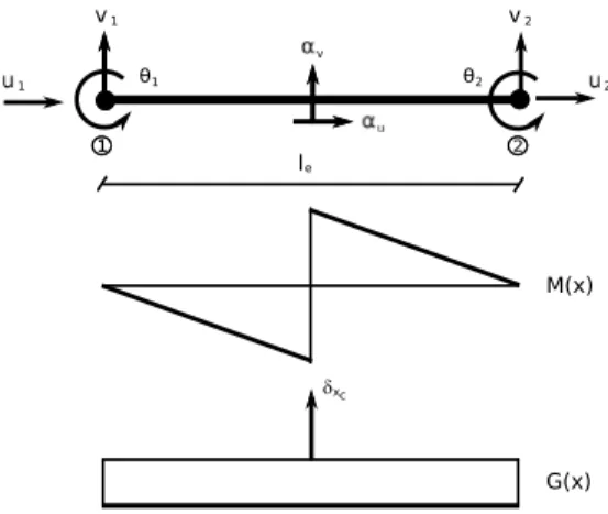
Next we give the formulation for 2D Timoshenko beam element enhanced with embedded strong discontinuity, which is capable to provide failure mechanisms and corresponding displacement jump inside the element (Fig. 1.c). The occurrence of jump in the displacement field is followed by softening plasticity behavior. One can trigger jump in normal displacement for mode I and transverse displacement for mode II.

2.1. Enhanced kinematics of 2D Timoshenko beam element

One can start from standard kinematics of a geometrically linear Timoshenko beam finite element of length leand

cross section A = h · 1 in order to obtain the strain measuresϵ

ϵ(x) = ⎡ ⎢ ⎢ ⎢ ⎢ ⎣ ϵ(x) = du d x γ (x) = dv d x −θ κ(x) = dθ d x ⎤ ⎥ ⎥ ⎥ ⎥ ⎦ (1)

where u = [u v θ]T _{is the generalized displacement vector with longitudinal displacement, transverse displacement}

and rotation as shown inFig. 2andϵ = [ϵ γ κ]T is a corresponding strain vector.

In order to represent the mode I as axial failure and mode II failure as shear failure, we introduce discontinuities in the generalized displacement field of the 2D Timoshenko beam. This is achieved with Heaviside function Hxcdefined

by Hxc(x) = 0 for x ≤ xcand Hxc(x) = 1 and vectorα = [αu αv 0]

T _{which represents the vector of displacement}

jumps at the point of discontinuity xc placed in the middle of the beam. The position of discontinuity corresponds

to intersection of the neighboring Voronoi cells (Fig. 1.c). The embedded strong discontinuity inside element will allow to provide mesh independent response in terms of energy for softening law. More precisely, fracture energy as input parameter will remain independent on mesh. We can write the displacement field as the sum of continuous displacement and a displacement jump as

u(x) = u(x) +αHxc = ⎡ ⎣ u(x) v(x) θ(x) ⎤ ⎦ + ⎡ ⎣ αu αv 0 ⎤ ⎦ Hxc. (2)

Fig. 2. Timoshenko beam with standard degrees of freedom and additional ones related to jumps in the displacement fields. M(x) and G(x) are the discontinuity related additional enrichment functions.

Thus, Eq.(2) can be rewritten by adding and subtracting a regular differentiable function from Heaviside function (see [20] for more details) and the resulting finite element interpolations for displacement field can be recast as

u(x) = N1(x)u1+N2(x)u2+α (Hxc−N2(x))

  

M(x)

(3)

where regular part of Timoshenko beam displacements is interpolated with shape functions as linear polynomials, N1(x) = 1 −_lx

e, N2(x) =

x

le. An additional discontinuity-related unknown is accompanied by enrichment function for

displacement field denoted as M

M(x) = {− x le ;x ∈[0, xc⟩ 1 − x le ;x ∈ ⟨xc, le]. (4)

The function M(x) (seeFig. 2) is an element enrichment function, containing element unit jump function, which characterizes the embedded discontinuity approach where the contribution of the discontinuity will cancel at element nodes leaving only standard nodal unknowns. Moreover, additional discontinuity degrees of freedomα can be kept inside the element, which are solved for at the element level by computation that are independent on the global finite element procedure. We can write the enhanced total displacement field in a matrix form as

u = Nua+Mα (5)

with N as 3 × 6 matrix containing element shape functions N1(x) and N2(x), and M is 3 × 3 matrix containing

discontinuity interpolation functions M positioned at the first two diagonal entries related to translational degrees of freedom, leaving rotation interpolation intact.

Interpolation of enhanced strain field requires the derivatives of shape functions B1(x) = −_l1

e, B2(x) =

1

le and the

derivative G of enrichment M, leading to

G(x) = G(x) +δxc, G(x) = −

1 le

. (6)

The function G is split into regular part G and singular part in terms ofδxc. The expression above reduces to

G(x) = −B2(x). The interpolated enhanced strain field can be obtained with

ϵ = Bua+Gα + αδxc (7)

where B is 3 × 6 beam strain–displacement matrix corresponding to Eq.(1)and G is the 3 × 3 matrix of derivatives of discontinuity enriched function G at the entries related to translational degrees of freedom.

2.2. Variational equation

The virtual strain field can be constructed in the same way as real enhanced strain field

δϵ = Bδua+Gvδα + δαδxc (8)

whereδuaandδα represent virtual displacement field and virtual displacement jump. We can build the virtual work

equation Gi nt,(e)−Gex t,(e)=0, where internal work is defined as Gi nt,(e)=∫le

0 (δϵ)

T_{σdx. The finite element assembly}

procedure with enhanced elements produces the two groups of equations Anel e=1(f i nt,(e)_−fex t_{) = 0} h(e)= ∫ le 0 GTσdx + t, ∀e ∈ [1, nel]. (9)

The first of these is a set of global equations where fi nt,(e)₌∫le

0 B

T_{σdx. The second equation with condition h}(e)₌₀

needs to be enforced in each element where discontinuity is activated, which leads to definition of the traction vector at discontinuity

t = − ∫ le

0

Gσ dx. (10)

Note that assembly operator in the first equation in(9)considers all elements, while the second equation remains limited to a particular element due to character of interpolation function for discontinuity which takes zero values at the element boundary.

In order to solve the nonlinear problem addressed in Eq.(9), the consistent linearization (e.g. see [1]) of both equations has to be performed. The standard Newton incremental-iterative procedure is used to provide new iterative values of nodal displacements

Anel

e=1

[

K_n+1e,(i)∆u(i )_n+1+F_n+1e,(i)∆α(i )_n+1]=Anel

e=1

[

fex t_n+1,e−fi nt_n+1,e,(i)] h_n+1e,(i)+(F_v,n+1e,(i) +K(i )_d,n+1)∆u_n+1(i ) +(He_n+1,(i)+K(i )_α,n+1)∆α(i )_n+1=0

(11)

where the explicit form of matrices is

Ke_n+1,(i)= ∫ le 0 BTC(i )_n+1Bd x, Fe_n+1,(i)= ∫ le 0 BTC(i )_n+1Gd x Fe_v,n+1,(i) = ∫ le 0 GTC(i )_n+1Bd x, He_n+1,(i)= ∫ le 0 GTC(i )_n+1Gd x (12)

and C(i )_n+1 =di ag(E A, G A, E I ) is the tangent stiffness for 3D Timoshenko beam. Similarly, K(i )_d,n+1and K(i )_α,n+1are the consistent tangent stiffness for discontinuity

∆t(i )_n+1=K(i )_d,n+1∆u_n+1(i ) +K(i )_α,n+1∆α(i )_n+1. (13) Enforcement of the local equation in(9) allows us to exploit the static condensation of the additional degrees of freedom (e.g. [1]). This leads to the reduced size of stiffness matrix corresponding to global unknowns only, which is calculated as follows:

ˆ

Ke_n+1,(i)=Ke_n+1,(i)−Fe_n+1,(i),T(He_n+1,(i)+K_α,n+1(i ) )−1(F_v,n+1e,(i) +K_d(i )_,n+1). (14) A reduced stiffness matrix contributes to finite element assembly procedure to provide global set of linearized equilibrium equations. Computed incremental displacements ∆u(i )_n+1are used to perform corresponding displacement vector update Anel e=1Kˆe_n+1∆u (i ) n+1= A n_el e=1 [ fex t_n+1,e−fi nt_n+1,e,(i)] H⇒u(i +1)_n+1 =u(i )_n+1+∆u(i )_n+1. (15)

2.3. Extension to dynamics

Since embedded discontinuity contribution is kept at the element level with internal force vector fi nt_n+1,e,(i)contained inside an element, one can easily extend the proposed approach to the dynamics framework by applying the d’Alembert principle to the system of equations written above. By applying the standard finite element interpolations and assembly procedure, classical global system of equations of motion Man+1+fi ntn+1=f

ex t

n+1is obtained. Global mass

matrix M = Anel

e=1Me is assembled from element mass matrices Me =

∫le

0 N

T_{ρ ANdx, where ρ represents material}

density and A beam cross section. Vector an+1contains nodal accelerations.

One can apply the classical implicit Newmark scheme to solve the corresponding dynamics equation of motion. The displacement and velocity updates can be expressed in terms of Newmark’sβ and γ parameters as

un+1=un+∆t vn+(∆t )2 [ (1 2−β)an+βan+1 ] vn+1=vn+∆t[(1 −γ )an+γ an+1 ] (16)

where ∆t is increment in time. In order to solve nonlinear equations of motion, we can first combine Eqs.(16)to obtain an+1 an+1= − 1 2−β β an− vn β∆t + 1 (∆t )2β(un+1−un). (17)

The linearization procedure on the result in (17) will provide the possible iterative improvement and updates un+1=u(i )_n+1+∆u(i )_n+1. The insertion of linearized equation(17)into equations of motion will produce the following

system of equations which can be solved by Newton procedure:

Anel e=1 ( ₁ (∆t )2βM e₊ ˆ Ke_n+1 ) ∆u(i )_n+1= Anel e=1 [ fex t_n+1,e−fi nt_n+1,e,(i)−Mea(i )_n+1] H⇒u(i +1)_n+1 =u(i )_n+1+∆u(i )_n+1. (18)

It is important to note that embedded discontinuity is confined in internal force vector and that statically condensed stiffness matrix still remains the same like in quasi-static case. Moreover, the corresponding extension for dynamic crack propagation can be performed just by adding inertial terms on top of existing formulation for quasi-static case. Here, we use Newmark’s parametersβ = 1/4 and γ = 1/2 and Newton’s algorithm with line search to obtain the corresponding displacement update and solution of nonlinear system. Note that we did not have to use any additional damping matrix or other similar contribution.

2.4. Plastic softening

Internal force vector in(9)in a beam lattice contains stress resultantsσ = [N V M]T, where axial and shear are computed with softening plasticity as a result of occurrence of failure modes I and II activated upon reaching failure threshold. The response to rotation is kept linear elastic. The evolution of softening plasticity variables is governed by singular part of deformation field at the position of discontinuity, while stress field remains smooth [8]. The computation of vectorσ can be split into two scalar equations, where each failure mode appears separately. In order to simplify the following presentation, we will write the scalar equations, which are valid for computation of both failure modes and corresponding stress resultants in axial and transverse directions. Here we start with a Helmholtz free energy potential for softening plasticity

Ψ (σ, q) = 1 2σ ϵ e    Ψel +Ξ (ξ)    Ψpl ; Ξ (ξ) = −qξ (19)

whereξ represents internal softening variable, ϵeis elastic strain and q is a stress-like softening variable defined with exponential softening constitutive law for discontinuity

q =σu ( 1 − ex p ( −ξ σu Gf )) (20)

Gf is the corresponding value of fracture energy representing input parameter,σuis the failure threshold for mode I.

We useτuas a threshold for mode II. We can write the failure detection function for softening as

Φ(t, q) = t − (σu−q) ≤ 0 (21)

where t is a traction acting at the discontinuity computed from(10).

The evolution equations for discontinuity can be written similarly to standard plasticity with the main difference that the plastic deformation in softening remains localized at the particular point (represented by the Dirac function)

˙ α = ˙λ∂Φ ∂σ = ˙λsign(σ) ˙ ξ = ˙λ∂Φ_∂q = ˙λ (22)

whereλ is the plastic multiplier associated with the softening behavior and α is equivalent to the accumulated plastic strain at the discontinuity. The plastic dissipation in softening plasticity can be obtained with the second law of thermodynamics and written in a distributional sense. Its local form is given as (see also [8])

˙ DP =σ ˙ϵ − d dtΨ (σ, q) = [sign(σ ) + q(ξ)]   σu ˙ ξ. (23)

The total energy balance involving first and second laws of thermodynamics in any finite element elastoplastic model is given as

Wi nput =EK+ES+ EP+DP

  

Plastic Work WPl

(24)

where Wi nput is the total input work introduced into the system, EK is kinetic energy, ES strain energy, EP plastic

free energy and DP is energy dissipation due to plasticity. Note that ESand EPcorrespond to elastic and plastic parts

of free energy Ψel and Ψpl, respectively, defined by softening plasticity potential from(19). As indicated in [36], it is important to distinguish between energy dissipation DP and plastic work WPl, where plastic work represents

the combination of plastic dissipation and plastic free energy. Namely, only one part of this non-recoverable plastic work is dissipated and converted into heat. The remaining part of the plastic work, also known as stored energy of cold work, is stored as internal energy and occurs as a consequence of rearrangement of microstructural crystals [37]. Details on energy dissipation analysis in various plasticity hardening models can be found in [36].

Energy balance equation(24) can also be recovered by using the theorem of expended stress power (see [8]) combined with energy dissipation which states

˙ DP = ˙Wi nput− d dt [∫ Ω Ψ dΩ ] − d dt [∫ Ω eKdΩ ] . (25)

Note that ˙DP is a rate of dissipation. ˙Wi nput represents the rate of input work which is equal to internal stress power.

If we rewrite equation(25)and decompose free energy Ψ into elastic and plastic parts, being strain and plastic free energy densities eSand eP respectively, with kinetic energy density eK, we obtain

˙ Wi nput = d dt [∫ Ω eKdΩ ] + d dt [∫ Ω eSdΩ ] + d dt [∫ Ω ePdΩ ] + ˙DP. (26)

Integration over time of(26)will provide energy balance equation(24)and the total values for energy components ∫ t t0 ˙ Wi nputdt    Wi nput = ∫ t t0 d dt [∫ Ω eKdΩ ] dt    EK + ∫ t t0 d dt [∫ Ω eSdΩ ] dt    ES + ∫ t t0 d dt [∫ Ω ePdΩ ] dt    EP + ∫ t t0 ˙ DPdt    DP . (27)

Here we deal with elastoplastic softening model where energy balance must be satisfied. It is important to emphasize that energy dissipation must always be positive, while plastic free energy need not be. In softening regime, the integral of plastic free energy will become negative (due to negative sign in free potential). Then, the sum of total dissipation and negative plastic free energy will result in the amount of plastic work.

In our analyses, we will plot the values of plastic work because it represents the area under the softening curve. Moreover, integration of plastic work across the fracture zone to infinity allows us to recover the fracture energy needed to drive the material until the total failure (see [1,8])

Gf = ∫ ∞ 0 σuex p ( −ξ σu Gf ) dξ. (28)

Note that the plastic work (combination of plastic dissipation and plastic free energy) is computed by above integral (28) in the limits up to the current time step. That integral is solved analytically in our code. The final analytically integrated expression for total plastic work from beginning of the simulation up to the current time step is WPl =Gf

(

1 − ex p(−σu

Gfξb

))

, withξbbeing the value of internal variable at the current time step.

The computational procedure for calculation of discontinuity variables and stress is similar to return mapping algorithm of standard hardening plasticity. Trial values of failure function and traction acting at the discontinuity are computed in order to check if the failure occurred or not. If yes, internal variables of discontinuity are updated and traction is computed with updated internal variables. The details can be found in [1,18–20].

Since the normal and the shear force (mode I and mode II failure also) in the Timoshenko beam are uncoupled, we need to define the failure surfaces for both directions and check them separately. The computational algorithm is thus performed for both modes independently using axial and shear stiffnesses of the beam. Here, we take the two trial failure surfaces for detection of failure modes I and II

Φ_utr i al_,n+1=t_utr i al_,n+1−(_σ u−qu,n ) Φ_v,n+1tr i al =⏐⏐t_v,n+1tr i al ⏐⏐ − (_τ u−qv,n ) (29)

whereσuandτuare failure thresholds for mode I and II and n denotes time step.

3. Enhanced solid model with embedded strong discontinuities

The proposed solid model, based on triangular constant strain finite elements with embedded strong discontinuities has already been developed for quasi static failure of solids [15]. It has also successfully been used to account for dynamic effects under slowly increasing loads in [16]. The inertial effects were shown to reduce the number of iterations and to increase computational robustness, especially with complex crack paths. In the present paper we subject the developed model to the well known benchmarks for dynamic crack propagation in which fast dynamics and significant inertial forces drive the specimen failure mechanisms.

Enrichment procedure resulting with embedded strong discontinuity in the solid element is in principle similar to the one presented above in the discrete lattice model. The main difference pertains to triangular constant strain finite element and 2D enhancement functions related to discontinuity in contrast to those presented in lattice model, which were 1D shape functions for Timoshenko beam. Another difference in the two presented models is that constitutive law for discontinuity exhibits damage softening behavior, in contrast to plasticity softening presented in lattice model. However, the distinction between damage and plasticity becomes pronounced when one goes through unloading and cyclic loading [1], which is not the case of the main interest in this work. Thus, we can compare the performance of these two models in crack propagation problems and also collect the common conclusions and characteristics of the embedded strong discontinuity approach.

Next we briefly present the main ingredients of the formulation for enhanced triangular finite element with embedded discontinuity, which again allows for the condensation of additional degrees of freedom before proceeding towards the solution at the global level. We also show that global tracking algorithm is not necessary neither in this model.

3.1. Enhanced kinematics

The embedded strong discontinuity for localized failure representation in solid element is obtained by introducing the displacement jump with Heaviside function in the total displacement field

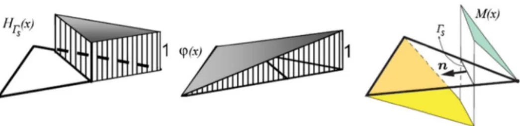
Fig. 3. Discontinuous shape function (2D case) for a CST element with constant discontinuity jumps.

where ¯¯u denotes displacement jump and Heaviside function is defined as

HΓs(x) =

{1 x ∈∂Ω−

0 x ∈∂Ω+ (31)

with∂Ω−_and∂Ω+_{are the boundary of the two sub-domains separated by discontinuity. The enhanced strain can be}

computed from displacement field as sum of regular continuous part and discontinuous part as

ϵ(x, t) = ¯ϵ(x, t) + ¯¯ϵ(x, t)δΓs(x) (32) where ¯ ϵ(x, t) = ▽s_{u(x, t) + H¯} Γs▽ s_{¯¯u(x, t)} ¯¯ ϵ(x, t) = (¯¯u(x, t) ⊗ n)s (33)

and n is a normal vector to discontinuity line (seeFig. 3) The finite element interpolation for a triangular CST element in which the displacement jump is taken as constant can provide the interpolated total displacement field

u(x, t) =ˆu(x, t) + ¯¯u(x, t) [HΓs(x) −ϕ(x)] (34)

where_ˆu(x, t) represents the classical displacement interpolation of a CST from which we can get the regular strain field as_ˆu(x, t) = Nua. By introducing an additional shape function M(x) = HΓs(x) −ϕ(x) shown inFig. 3and its

derivative G, we can obtain interpolated real strain and virtual strain field

ϵ(x, t) = Bd + Gr¯¯u H⇒∂ϵ(x, t) = Bw + Gvβ¯¯ (35)

B stands for a matrix form of the strain–displacement operator ∇s_{, G}

vis referred to as an incompatible mode function

modified so that it can fulfill the patch test condition, whileβ and w are respectively, displacement jump and virtual¯¯ displacement field.

3.2. Linearization of virtual work

The virtual work equation is established from enhanced real and virtual strain fields like in the discrete lattice model described above. Here, we give the assembled virtual work equations with included mass terms and inertial effects ⎧ ⎪ ⎨ ⎪ ⎩ r(e)_n+1,(i)_{= A}nel e=1 [

f(e)_{ex t},(i)_,n+1−f(e)_{i nt},(i)_,n+1−Ma(e)_n+1,(i)] f or x ∈Ω \ Γs

h(e)_n+1,(i)= ∫ Ωe ¯ G_vTσ(e)_n+1,(i)dΩe+ ∫ Γs ¯¯ GT_vtΓsdΓs =0 f or x ∈Γs. (36)

In order to solve this system of nonlinear equations, we perform the consistent linearization (see [1]) which results with [ Ane=1el ˆKe A nel e=1F e F(e),T H(e) ]i n+1 ( ∆d(e)_n+1,(i) ∆ ¯¯u(e)_n+1,(i) ) = ( Ane=1el r (e)_,(i) n+1 h(e)_n+1,(i) ) . (37)

The embedded strong discontinuity approach allows to exploit the condensation of discontinuity related parameters producing the final linearized equation

Ane=1el (K (e)_,(i) e f f,n+1∆d (e)_,(i) n+1 ) = A nel e=1r (e)_,(i) e f f,n+1. (38)

The effective matrix K(e)_{e f f},(i)_,n+1contains the contribution from static condensation due to embedded strong discontinuity, where element sub-matrices H(e) _{and F}(e) _{are computed in a similar manner to the one presented in Section 2.}

Additionally, the effective matrix also contains the contribution from the Newmark algorithm for time integration in dynamics K(e)_{e f f},(i)_,n+1=ˆK (e),(i) n+1 −F (e),(i) n+1 (H (e),(i) n+1 ) −1_F(e),(i),T n+1 + 1 (∆t )2βM e ₍₃₉₎

and residual is computed by subtracting the inertial terms

r(e)_{e f f},(i)_,n+1=r(e)_n+1,(i)−Me_a(i )

n+1. (40)

3.3. Damage softening

The occurrence of localized failure in enhanced CST element is followed by damage softening constitutive law for crack opening. The model is also developed so that it can account for damage hardening behavior, which is summarized in free energy potential defined as

ψ(ϵ, D, ξ) = 1 2ϵ · ¯D¯ −1_{ϵ + ¯Ξ (¯ξ)¯}    ¯ ψ(¯ϵ, ¯D,¯ξ) +1 2¯¯u · ¯¯Q −1 ¯¯u +Ξ (¯¯ξ)¯¯    ¯¯ ψ(¯¯u,¯¯Q,¯¯ξ) δΓs. (41)

We can note that free energy is split into two parts, where the first one concerns the hardening part and the second one softening localized part which is introduced by Dirac function. In this work we are interested in localized softening part only which occurs when the failure is detected by damage softening functionΦ = 0, with no hardening. Here,¯¯

¯¯

Ξ (¯¯ξ) = − ¯¯q ¯¯ξ and stress-like damage softening variable is defined as exponential function ¯¯ q = ¯¯σf [ 1 − ex p(− ¯¯ β ¯¯ σf ¯¯ξ) ] H⇒K = −¯¯ ∂ ¯¯q ∂¯¯ξ = −βexp(−¯¯ ¯¯ β ¯¯ σf ¯¯ξ). (42)

The softening detection function is defined as ¯¯

Φ(tΓs, ¯¯q) =Φ(tˆ¯¯ Γs) − ( ¯¯σf − ¯¯q) (43)

whereΦ(tˆ¯¯ Γs) is a function of degree one containing the traction vector tΓs = (σn)Γs which acts at discontinuity

surface. We can write the loading–unloading conditions and consistency condition

˙¯¯γ ≥ 0 Φ(t˙¯¯ Γs, ¯¯q) ≤ 0 ˙¯¯γΦ(t˙¯¯ Γs, ¯¯q) = 0. (44)

The damage dissipation in localized softening can be defined as

˙ DP = 1 2tΓs · ˙¯¯ Q t_Γ s − dΞ (¯¯ ¯¯ξ) d¯¯ξ ˙¯¯ξ = 1 2tΓs · ˙¯¯ Q t_Γ s + ¯¯q˙¯¯ξ. (45)

Similarly to plasticity case described above, the integration of the theorem of expended stress power provides the value for fracture energy

Gf = ∫ ∞ 0 ¯¯ σfex p(− ¯¯ β ¯¯ σf ¯¯ξ)d ¯¯ξ (46)

while damage work WDcan be obtained by integrating the expression(46)in the range from zero to current value

Fig. 4. Set up for Kalthoff’s experiment.

4. Numerical simulations

In this section we present the results of numerical simulations. Each simulation deals with problem where localized failure with crack initiation and propagation is triggered by impulsive load and where the inertial effects are important. The presented examples include some demanding problems, including Kalthoff’s experiment in which plate with two notches is subjected to edge impact [38] and dynamic crack branching problem [39]. Simulations are conducted with both models presented above, which are implemented into research version of the computer code FEAP [40].

4.1. Pre-notched plate subjected to impulsive load—kalthoff ’s experiment

In this test, the two notched maraging steel specimen is subjected to the edge impact of a projectile applied in the direction of the notches (seeFig. 4). The available experimental results for such test, reported in Kalthoff [38] (with variation of this test with one notch in Zhou et al. [41]), attracted large interest turning this example into the benchmark. Namely, numerical computations for the test are conducted with various methods such as XFEM [3–5], ED-FEM [9,10], phase field [11,12] or discrete lattice model [32,33].

Geometry and boundary conditions of the specimen are given inFig. 4. The projectile impact is represented in the model by imposed velocity, which is initially applied and held constant. We can consider here only half of the mesh due to the symmetry in order to reduce the computational cost. The initial notch is modeled directly by leaving the space in the mesh. The material parameters for maraging steel are chosen for model parameters withρ = 8000 kg/m3_,

E = 190 GPa andν = 0.3. The maximal uniaxial tensile stress of σu =1.07 GPa is considered for threshold value

which triggers the failure mechanism in mode I. The other model parameters are fracture energy in mode I chosen as Gf,I =5 × 104 N/m for plasticity model and softening variable βI =17 GPa/mm chosen for the damage model.

We also consider the possible failure in mode II, with model parameters for shear threshold value chosen asτu =1

GPa, fracture energy for mode II in plasticity model Gf,I I =5 × 104 N/m and damage model parameter βI I =17

GPa/mm.

When subjected to edge impulsive load, the maraging steel exhibits failure mode transition. Namely, for lower loading rates, failure is influenced by mode I tensile crack at an angle of about 70◦. High loading rates on the contrary produce failure in mode II by adiabatic shear bands which are experimentally observed in [38].

First we model the case with lower loading rate where we impose constant velocity ofv0=16.5 m/s at the position

of projectile impact. Three different mesh densities are used for the same experiment and with both models. It should be noted that elements in discrete lattice model mesh are Timoshenko beams, which are positioned at Delaunay edges

Fig. 5. Crack opening [mm] at the end of simulation time with discrete lattice model for (a) Mesh1, (b) Mesh2 (c) Mesh3; applied impact velocity isv0=16.5 m/s.

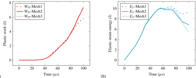
Fig. 6. Energy evolution with discrete lattice model for applied impact velocityv0=16.5 m/s: (a) plastic work versus time (b) elastic strain energy

versus time.

from triangulation. Three different meshes are used, named Mesh1, Mesh2 and Mesh3 representing coarse, medium and fine mesh. They result with 2122, 6732 and 17 629 Timoshenko beam lattice elements, respectively. The three corresponding meshes for enhanced solid model are composed of 1383, 4421 and 11 649 triangular elements for coarse, medium and fine mesh.

Fig. 5shows the contour plot obtained with discrete lattice model for low loading rate impact. It can be observed that for all mesh densities, the main crack propagates from the top of the notch at an angle of about 70◦_{, the same as}

observed in experiment. The simulation is run for 100 µs and the crack propagated to similar position in all three cases. It is worth noting that this crack is governed dominantly by tensile failure and failure function for mode I activated the embedded discontinuity and strain softening behavior inside failing elements. Since no tracking algorithm has been used to enforce only one crack, secondary crack propagated in the lower right corner of the specimen. The cracks are propagated by the stress concentration at the crack tip, while stress distribution governed the failure direction. Continuity of the crack was preserved without enforcing it with tracking algorithm.

Figs. 6and7reveal energy balance for the failure obtained with discrete lattice model. Firstly, the plastic work and elastic strain energy are plotted with respect to time inFig. 6. Since embedded discontinuity and corresponding element enrichment procedure provide the possibility of failure mechanism inside elements with mesh independent softening response, plastic work also remains mesh independent. We can observe fromFig. 6.a that the plastic work in all three meshes remains very close, since cracks propagated until the same position in the mesh and localized failure occurred in the interiors of lattice elements. The minor perturbation in plastic work is produced by the secondary

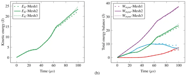
Fig. 7. Energy evolution with discrete lattice model for applied impact velocityv0 =16.5 m/s: (a) kinetic energy versus time (b) total energy

balance versus time (purple—total input work, red—plastic work, blue—elastic strain energy, green—kinetic energy). (For interpretation of the references to colour in this figure legend, the reader is referred to the web version of this article.)

Fig. 8. Crack opening [mm] at the end of simulation time with enhanced triangle model for (a) Mesh1, (b) Mesh2, (c) Mesh3; applied impact velocity isv0=16.5 m/s.

crack in coarse mesh, which propagated in slightly different manner in the later stage of simulation. This can be explained by microstructural difference in coarse mesh, where indeed the irregular grid introduces small perturbation and crack always propagate through the weakest links among adjacent ones. The elastic strain energy computed from elastic strain follows the similar pattern inFig. 6.b, except that coarse mesh reaches slightly higher peak value.

Fig. 7.a shows kinetic energy evolution in time for all meshes, which is computed as K = 1₂vn+1Mvn+1, with v

being velocity vector and M mass matrix. The total energy balance is plotted inFig. 7.b, where the sum of plastic work (combination of plastic free energy and dissipation), strain and kinetic energy in every time step equals the total input work introduced into the system by external loads. The total input work on the boundary can be computed as Wi nput = ∑

nst ep

n=1 Fn+1/2·∆uΓ, with Γ denoting the boundary. Computation of total input work also provides the

possibility to verify all the internal energy components.

The mode I dominated crack was also obtained with enhanced triangular solid model, where failure function for tensile crack opening governed the crack propagation.Fig. 8shows the failure pattern for all three meshes. Although the cracks appear to be thicker for coarse mesh, it is only the consequence of smoothening in post-processing on a larger grid. In fact, the three failure mechanism remains localized inside elements. This is generally the characteristics of embedded discontinuity way of enrichment, which is confirmed here with two different models. The main crack remains at the similar angle for all meshes, while secondary crack emerged again from the lower right angle. The tracking algorithm was not needed with enhanced solid model, since the stress concentration at the crack tip naturally propagated the crack preserving the continuity. The plots for damage work and elastic strain energy are given inFig. 9.

Fig. 9. Energy evolution with enhanced triangle model for applied impact velocityv0=16.5 m/s: (a) damage work versus time (b) elastic strain

energy versus time.

Fig. 10. Energy evolution with enhanced triangle model for applied impact velocityv0=16.5 m/s: (a) kinetic energy versus time (b) total energy

balance versus time (purple—total input work, red—damage work, blue—elastic strain energy, green—kinetic energy). (For interpretation of the references to colour in this figure legend, the reader is referred to the web version of this article.)

The curves for damage work obtained with enhanced triangular solid model in different meshes remain fairly close. The main distinction with respect to the results obtained with discrete lattice model is that for such chosen damage parametersβI andβI I, damage work is much less pronounced in triangular damage model. Elastic strain energy is

also slightly different with respect to plasticity model, due to less damage work. Kinetic energy and total energy balance obtained with damage model are shown inFig. 10.

Next, we apply the higher rate of impact load to the same specimen, with imposed velocity ofv0 =50 m/s. The

results obtained with discrete lattice model are presented inFig. 11. One can note fromFig. 11.a and b that impact experiment now results in a completely different failure behavior, with crack propagating straight from the notch horizontally and curving a little bit near the end of the specimen. It is the mode II dominated crack, where failure function for shear governed the propagation of the crack. This is in agreement with experimental result observed from [38], where high rates of loading cause adiabatic shear band and failure due to sliding in maraging steel specimens. It is also confirmed experimentally that development of shear band requires and absorbs more energy than in tensile failure pattern. This fact has been recovered with our model where plastic work and elastic strain energy reach higher values (seeFig. 11.c) than in the previous test. The high rate loading test was conducted with Mesh1 and Mesh2. The

Fig. 11. Adiabatic shear band development with discrete lattice model for impact velocity ofv0=50 m/s: (a) shear band sliding [mm] (Mesh1)

(b) shear band sliding [mm] (Mesh2) (c) total energy balance.

Fig. 12. Set up for crack branching experiment.

crack path is not identical in two meshes as a consequence of small perturbation in irregular mesh. All the components of energy confirm this variation.

Adiabatic shear band could not be obtained with enhanced triangular solid element, since the crack got arrested immediately at the beginning of the simulation. The same was observed in experiment where shear failure gets arrested in most of the cases and applied velocities. Different thicknesses of the notch are also varied in experiment. The shear failure also got arrested with the discrete lattice model in the range of imposed velocities betweenv0 =30 m/s and

v0=50 m/s.

4.2. Crack branching experiment

The next simulations are conducted to obtain the crack branching phenomena, which is experimentally observed in [39]. Numerical simulations of the branching experiment with various models are reported in [5,9,10,32] among others. A pre-notched square plate is subjected dynamically to tension load. The geometry and loading conditions are shown inFig. 12. The chosen values of model material parameters are E = 3.24 GPa,ν = 0.35, ρ = 1.19 g/cm3_and

the mean value of ultimate tensile failure threshold isσu =129 MPa, with standard deviation of 2%. The fracture

energy for mode I in plasticity model is Gf,I =4 × 103N/m, while corresponding parameter for damage softening

model isβI = 35 GPa/mm. Two meshes, one with 4400 (Mesh 1) and the other with 5885 (Mesh 2) Timoshenko

beam elements were used in discrete lattice model simulations, while the solid element mesh corresponding to Mesh 1 results with 2891 triangular elements.

We show that embedded discontinuity formulation can also be used to obtain branching of the main crack among other complex crack patterns, without using global crack tracking procedure or additional crack branching criterion. We applied two imposed velocities (v0 = 7 m/s and v0 = 11 m/s) on top and bottom of the square specimen.

Fig. 13. Crack branching test (Mesh 1): Crack opening [mm] at the end of simulation time with discrete lattice model (a)v0=7 m/s, (b) v0=11

m/s.

Fig. 14. Crack branching test (Mesh 2): Crack opening [mm] at the end of simulation time with discrete lattice model (a)v0=7 m/s, (b) v0=11

m/s.

Figs. 13–15show the contours of the specimen and corresponding opening of the crack obtained with discrete lattice and enhanced solid element, respectively. One can observe that the crack path is not identical in all cases. Moreover, crack is propagated as a consequence of material structure which is defined here by applied heterogeneity.

All the presented computations (Kalthoff’s test and crack branching test) have been conducted on a single core processor with FEAP software. The increment of time is taken to be ∆t = 1 µs for all computations. The convergence between internal and external force vector of implicit dynamic nonlinear solver in a typical time step, with propagating crack, is reached within 10 iterations. More demanding time step, including significant stress redistributions and failure of multiple adjacent elements that simultaneously enter softening phase, is typically converged within 20 iterations. The Newton nonlinear solver is combined with line search technique to increase robustness. CPU time (discrete lattice model) required for full simulation of Kalthoff’s test with impact velocityv0 = 16.5 m/s is 208 s

(Mesh1), 8446 s (Mesh2) and 154 600 s (Mesh3). Kalthoff’s test simulation with impact velocityv0 =50 m/s is run

for 431 s (Mesh1) and 16 289 s (Mesh2). Crack branching test simulation forv0=7 m/s is finished in 2235 s (Mesh1)

and 4591 s (Mesh2).

5. Conclusions

We developed and validated against experiments two models for crack propagation in dynamics framework. Both models are based on embedded strong discontinuity finite element approach. The first model is based on Timoshenko

Fig. 15. Crack branching test: Crack opening [mm] at the end of simulation time with enhanced triangle model (a)v0=7 m/s, (b)v0=11 m/s.

beam lattice extracted from Voronoi cells, where Timoshenko beams are equipped with embedded discontinuity enhancements to provide failure modes I and II. This model was developed in our earlier works for quasi-static failure in heterogeneous materials. Here, we show that extension to dynamics framework can be upgraded in a straightforward manner by adding the inertial contributions without need for changing the existing quasi static model. The second model is based on enhanced triangular solid element, where failure also occurs due to modes I and II. The extension to dynamics framework is performed in the same way, without any need to change the code for existing quasi static case. The presented two models are developed initially for failure in heterogeneous materials and solid structures, respectively.

We conducted the two dynamic crack propagation benchmarks with both models where we could summarize the features of the approach for crack phenomena based on embedded strong discontinuity. Namely, since contribution of embedded strong discontinuity enhancement remains local inside elements, different mesh sizes, and even fairly coarse grids, could be used to obtain results for presented dynamics benchmarks. The same approach allows to keep the fixed mesh during the whole simulation, due to crack propagating in the element interiors. These benefits lead to high computational efficiency. It is important to note that we did not use any tracking procedure for crack which would additionally increase the computational cost. Namely, tracking the crack path was not the major concern of this work. Instead, we rather focus upon the true energy balance and leave the material structure and complex stress states across the crack tip to govern the crack path. For instance, stress concentration occurring on the top of the notch and crack would trigger and extend the crack, while stress state and inertial forces orientate the crack in corresponding directions. Complexities, such as multiple cracks with their interaction, are shown to be represented very well. Dynamic crack branching phenomena can be obtained with both models. The tensile cracks are obtained in the so-called Kalthoff’s experiment where low rate of the impact load triggers the crack at an angle at about 70◦with both models. For high loading rate adiabatic shear band, or mode II crack, is obtained with discrete lattice model. However it could not be obtained with enhanced triangular solid model since the shear crack got arrested soon in the simulation.

The proposed methodology is computationally very efficient with various failure and crack related complexities being resolved. It can be used for computation of homogeneous solids and heterogeneous materials.

The true benefits of the approach could be used for failure applications in 3D environment where complex cracks become surfaces. Their interaction will automatically be resolved like shown in the present 2D case, while at the same time relatively coarse grids could provide correct failure phenomena all resulting with high computational efficiency.

Acknowledgments

Mijo Nikoli´c and ˇZeljana Nikoli´c would like to thank the Croatian Science Foundation for the funding of this work under the project Development of numerical models for reinforced-concrete and stone masonry structures under seismic loading based on discrete cracks(IP-2014-09-2319).

Xuan Nam Do and Adnan Ibrahimbegovic would like to thank the Hauts-de-France Region (CR Picardie) (120-2015-RDISTRUCT-000010 and RDISTRUCT-000010) and the European Regional Development Fund (ERDF)

2014/2020 for Chaire-de-Mecanique (120-2015-RDISTRUCTF-000010 and RDISTRUCTI-000004) for the funding of this work.

This support is gratefully acknowledged.

References

[1] A. Ibrahimbegovic, Nonlinear Solid Mechanics: Theoretical Formulations and Finite Element Solution Methods, Springer, London, 2009. [2] N. Moes, J. Dolbow, T. Belytschko, A finite element method for crack growth without remeshing, Internat. J. Numer. Methods Engrg. 46

(1999) 131–150.

[3] J. Rethore, A. Gravouil, A. Combescure, An energy-conserving scheme for dynamic crack growth using the eXtended finite element method, Internat. J. Numer. Methods Engrg. 63 (2005) 631–659.

[4] Z.L. Liu, T. Menouillard, T. Belytschko, An XFEM/spectral element method for dynamic crack propagation, Int. J. Fract. 169 (2011) 183–198. [5] T. Belytschko, H. Chen, J. Xu, G. Zi, Dynamic crack propagation based on loss of hyperbolicity and a new discontinuous enrichment, Internat.

J. Numer. Methods Engrg. 58 (2003) 1873–1905.

[6] N. Moes, T. Belytschko, Extended finite element method for cohesive crack growth, Eng. Fract. Mech. 69 (2002) 813–833.

[7] G. Ferte, P. Massin, N. Moes, 3D crack propagation with cohesive elements in the extended finite element method, Comput. Methods Appl. Mech. Engrg. 300 (2016) 347–374.

[8] J.C. Simo, J. Oliver, F. Armero, An analysis of strong discontinuities induced by strain-softening in rate-independent inelastic solids, Comput. Mech. 12 (1993) 277–296.

[9] F. Armero, C. Linder, Numerical simulation of dynamic fracture using finite elements with embedded discontinuities, Int. J. Fract. 160 (2009) 119–141.

[10] A.E. Huespe, J. Oliver, P.J. Sanchez, S. Blanco, V. Sonzogni, Strong discontinuity approach in dynamic fracture simulations, Mec. Comput. 25 (2006) 1997–2018.

[11] M.J. Borden, C.V. Verhoosel, M.A. Scott, T.J.R. Hughes, C.M. Landis, A phase-field description of dynamic brittle fracture, Comput. Methods Appl. Mech. Engrg. 217–220 (2012) 77–95.

[12] M. Hofacker, C. Miehe, A phase field model of dynamic fracture: Robust field updates for the analysis of complex crack patterns, Internat. J. Numer. Methods Engrg. 93 (2013) 276–301.

[13] J. Oliver, A.E. Huespe, P.J. Sanchez, A comparative study on finite elements for capturing strong discontinuities: E-FEM vs X-FEM, Comput. Methods Appl. Mech. Engrg. 195 (2006) 4732–4752.

[14] M. Nikolic, E. Karavelic, A. Ibrahimbegovic, P. Miscevic, Lattice element models and their peculiarities, Arch. Comput. Methods Eng. (2017). http://dx.doi.org/10.1007/s11831-017-9210-y.

[15] D. Brancherie, A. Ibrahimbegovic, Novel anisotropic continuum-discrete damage model capable of representing localized failure of massive structures, Eng. Comput. 26 (1/2) (2009) 100–127.

[16] X.N. Do, A. Ibrahimbegovic, D. Brancherie, Dynamics framework for 2D anisotropic continuum-discrete damage model for progressive localized failure of massive structures, Comput. Struct. 183 (2017) 14–26.

[17] A. Ibrahimbegovic, E. Wilson, A modified method of incompatible modes, Commun. Appl. Numer. Method 7 (1991) 187–194.

[18] M. Nikolic, A. Ibrahimbegovic, P. Miscevic, Brittle and ductile failure of rocks: Embedded discontinuity approach for representing mode I and mode II failure mechanisms, Internat. J. Numer. Methods Engrg. 102 (2015) 1507–1526.

[19] M. Nikolic, A. Ibrahimbegovic, Rock mechanics model capable of representing initial heterogeneities and full set of 3D failure mechanisms, Comput. Methods Appl. Mech. Engrg. 290 (2015) 209–227.

[20] E. Karavelic, M. Nikolic, A. Ibrahimbegovic, A. Kurtovic, A concrete meso-scale model with full set of 3D failure modes with random distribution of aggregate and cement phase. Part I: formulation and numerical implementation, Comput. Methods Appl. Mech. Engrg. (2017). http://dx.doi.org/10.1016/j.cma.2017.09.013.

[21] M. Nikolic, A. Ibrahimbegovic, P. Miscevic, Discrete element model for the analysis of fluid-saturated fractured poro-plastic medium based on sharp crack representation with embedded strong discontinuities, Comput. Methods Appl. Mech. Engrg. 298 (2016) 407–427.

[22] E. Hadzalic, A. Ibrahimbegovic, M. Nikolic, Failure mechanisms in coupled poro-plastic medium, Coupled Systems Mechanics 7 (1) (2018) 43–59.

[23] E. Schlangen, J.G.M. Van Mier, Simple lattice model for numerical simulation of fracture of concrete materials and structures, Mater. Struct. 25 (1992) 534–542.

[24] G. Cusatis, Z. Bazant, L. Cedolin, Confinement-shear lattice CSL model for fracture propagation in concrete, Comput. Methods Appl. Mech. Engrg. 195 (2006) 7154–7171.

[25] P. Grassl, M. Jirasek, Meso-scale approach to modelling the fracture process zone of concrete subjected to uniaxial tension, Internat. J. Solids Struct. 47 (2010) 957–968.

[26] M. Vassaux, C. Oliver-Leblond, B. Richard, F. Ragueneau, Beam-particle approach to model cracking and energy dissipation in concrete: Identification strategy and validation, Cem. Concr. Compos. 70 (2016) 1–14.

[27] B. Savija, J. Pacheco, E. Schlangen, Lattice modeling of chloride diffusion in sound and cracked concrete, Cem. Concr. Compos. 42 (2013) 30–40.

[28] A.S. Sattari, Z.H. Rizvi, H.B. Motra, F. Wuttke, Meso-scale modeling of heat transport in a heterogeneous cemented geomaterial by lattice element method, Granular Matter 19 (2017) 66.

[29] Z.H. Rizvi, D. Shrestha, A.S. Sattari, F. Wuttke, Numerical modelling of effective thermal conductivity for modified geomaterial using lattice element method, Heat Mass Transfer 54 (2) (2018) 483–499.

[30] B. Savija, E. Schlangen, On the use of a lattice model for analyzing of in-plane vibration of thin plates, Computers. Materials & Continua 48 (2015) 181–202.

[31] M. Attar, A. Karrech, K. Regenauer-Lieb, Non-linear modal analysis of structural components subjected to unilateral constraints, J. Sound Vib. 389 (2017) 380–410.

[32] M. Braun, J. Fernandez-Saez, A 2D discrete model with a bilinear softening constitutive law applied to dynamic crack propagation problems, Int. J. Fract. 197 (2016) 81–97.

[33] L. Kosteski, R.B. D’Ambra, I. Iturrioz, Crack propagation in elastic solids using the truss-like discrete element method, Int. J. Fract. 174 (2012) 139–161.

[34] G.A. D’Addetta, F. Kun, E. Ramm, H.J. Herrmann, From solids to granulates - Discrete element simulations of fracture and fragmentation processes in geomaterials, in: P.A. Vermeer, S. Diebels, W. Ehlers, H.J. Herrmann, S. Luding, E. Ramm (Eds.), Continuous and Discontinuous Modelling of Cohesive Frictional Materials, Springer, Berlin, 2001, pp. 231–258.

[35] A. Ibrahimbegovic, A. Delaplace, Microscale and mesoscale discrete models for dynamic fracture of structures built of brittle material, Comput. & Structures 81 (2003) 1255–1265.

[36] H. Yang, S.S. Sinha, Y. Feng, D.B. McCallen, B. Jeremic, Energy dissipation analysis of elastic-plastic materials, Comput. Methods Appl. Mech. Engrg. 331 (2018) 309–326.

[37] P. Rosakis, A.J. Rosakis, G. Ravichandran, J. Hodowany, A thermodynamic internal variable model for the partition of plastic work into heat and stored energy in metals, J. Mech. Phys. Solids 48 (2000) 581–607.

[38] J.F. Kalthoff, Modes of dynamic shear failure in solids, Int. J. Fract. 101 (2000) 1–31.

[39] K. Ravi-Chandar, W.G. Knauss, An experimental investigation into dynamic fracture: III On steady-state crack propagation and crack branching, Int. J. Fract. 26 (1984) 141–154.

[40] R.L. Taylor, FEAP Finite element Analysis Program. University of California, Berkeley,http://www.ce.berkeley.edu.rlt.

[41] M. Zhou, A.J. Rosakiss, G. Ravichandran, Dynamically propagating shear bands in impact-loaded prenotched plates - I. Experimental investigations of temperature signatures and propagating speed, J. Mech. Phys. Solids 44 (1996) 981–1006.