HAL Id: hal-01081186
https://hal.inria.fr/hal-01081186v2
Submitted on 22 Oct 2015HAL is a multi-disciplinary open access archive for the deposit and dissemination of sci-entific research documents, whether they are pub-lished or not. The documents may come from teaching and research institutions in France or abroad, or from public or private research centers.
L’archive ouverte pluridisciplinaire HAL, est destinée au dépôt et à la diffusion de documents scientifiques de niveau recherche, publiés ou non, émanant des établissements d’enseignement et de recherche français ou étrangers, des laboratoires publics ou privés.
Distributed under a Creative Commons Attribution - NonCommercial - NoDerivatives| 4.0
Georeplicated World
Roy Friedman, Michel Raynal, François Taïani
To cite this version:
Roy Friedman, Michel Raynal, François Taïani. Fisheye Consistency: Keeping Data in Synch in a Georeplicated World. [Research Report] 2022, IRISA. 2014. �hal-01081186v2�
PI 2022 – October 22, 2015
Fisheye Consistency: Keeping Data in Synch in a Georeplicated World
Roy Friedman* , Michel Raynal** ,*** François Taïani**
Abstract: Over the last thirty years, numerous consistency conditions for replicated data have been proposed and implemented. Popular examples of such conditions include linearizability (or atomicity), sequential consistency, causal consistency, and eventual consistency. These consistency conditions are usually defined independently from the computing entities (nodes) that manipulate the replicated data; i.e., they do not take into account how computing entities might be linked to one another, or geographically distributed. To address this lack, as a first contribution, this paper introduces the notion of proximity graph between computing nodes. If two nodes are connected in this graph, their operations must satisfy a strong consistency condition, while the operations invoked by other nodes are allowed to satisfy a weaker condition. The second contribution is the use of such a graph to provide a generic approach to the hybridization of data consistency conditions into the same system. We illustrate this approach on sequential consistency and causal consistency, and present a model in which all data operations are causally consistent, while operations by neighboring processes in the proximity graph are sequentially consistent. The third contribution of the paper is the design and the proof of a distributed algorithm based on this proximity graph, which combines sequential consistency and causal consistency (the resulting condition is called fisheye consistency). In doing so the paper not only extends the domain of consistency conditions, but provides a generic provably correct solution of direct relevance to modern georeplicated systems.
Key-words: Asynchronous message-passing system, Broadcast abstraction, Causal consistency, Data consistency, Data replication, Geographical distribution, Linearizability, Provable property, Sequential consistency.
La cohérence en œil de poisson : maintenir la synchronisation des données dans un monde géo-répliqué Résumé : Au cours des trente dernières années, de nombreuses conditions de cohérence pour les données répliquées ont été pro-posées et mises en oeuvre. Les exemples courants de ces conditions comprennent la linéarisabilité (ou atomicité), la cohérence séquentielle, la cohérence causale, et la cohérence éventuelle. Ces conditions de cohérence sont généralement définies indépen-damment des entités informatiques (noeuds) qui manipulent les données répliquées; c’est à dire qu’elles ne prennent pas en compte la façon dont les entités informatiques peuvent être liées les unes aux autres, ou géographiquement distribuées. Pour combler ce manque, ce document introduit la notion degraphe de proximité entre les noeuds de calcul d’un système réparti. Si deux noeuds sont connectés dans ce graphe, leurs activités doivent satisfaire une condition de cohérence forte, tandis que les opérations invoquées par d’autres noeuds peuvent ne satisfaire qu’une condition plus faible. Nous proposons d’utiliser un tel graphe pour fournir une approche générique à l’hybridation de conditions de cohérence des données dans un même système. Nous illustrons cette approche sur l’exemple de la cohérence séquentielle et de la cohérence causale, et présentons un modèle dans lequel, d’une part, toutes les opérations sont causalement cohérentes, et, d’autre part, les opérations par des processus qui sont voisins dans le graphe de proximité satisfont la cohérence séquentielle. Nous proposons et prouvons un algorithme distribué basé sur ce graphe de proximité, qui combine la cohérence séquentielle et la cohérence causal (nous appelons la cohérence obtenuecohérence en oeil de poisson). Ce faisant, le papier non seulement étend le domaine des conditions de cohérence, mais fournit une solution algorithmiquement correcte et générique directement applicable aux systèmes géo–répartis modernes.
Mots clés : Systèmes par passage de messages asynchrones, Abstractions de diffusion, Cohérence Causale, Cohérence des données, Réplication des données, Distribution géographiques, Linéarisabilité, Propriété prouvables, Cohérence Séquentielle
*
The Technion Haifa, Israel
**
Institut Universitaire de France
***
1
Introduction
Data consistency in distributed systems Distributed computer systems are growing in size, be it in terms of machines, data, or geographic distribution. Insuring strong consistency guarantees (e.g., linearizability [19]) in such large-scale systems has attracted a lot of attention over the years, and remains today a highly challenging area, for reasons of cost, failures, and scalability. One popular strategy to address these challenges has been to propose and implement weaker guarantees (e.g., causal consistency [2], or eventual consistency [38]).
These weaker consistency models are not a desirable goal in themselves [5], but rather an unavoidable compromise to obtain acceptable performance and availability [7, 12, 39]. These works try in general to minimize the violations of strong consistency, as these create anomalies for programmers and users. They further emphasize the low probability of such violations in their real deployments [14].
Recent related works For brevity, we cannot name all the many weak consistency conditions that have been proposed in the past. We focus instead on the most recent works in this area. One of the main hurdles in building systems and applications based on weak consistency models is how to generate an eventually consistent and meaningful image of the shared memory or storage [38]. In particular, a paramount sticking point is how to handle conflicting concurrent write (or update) operations and merge their result in a way that suits the target application. To that end, various conditions that enables custom conflict resolution and a host of corresponding data-types have been proposed and implemented [3, 4, 9, 13, 25, 29, 35, 34].
Another form of hybrid consistency conditions can be found in the seminal works on release consistency [17, 20] and hybrid consistency [6, 15], which distinguish between strong and weak operations such that strong operations enjoy stronger consistency guarantees than weak operations. Additional mechanisms and frameworks that enable combining operations of varying consistency levels have been recently proposed in the context of large scale and geo-replicated data centers [37, 39].
Motivation and problem statement In spite of their benefits, the above consistency conditions generally ignore the relative “distance” between nodes in the underlying “infrastructure”, where the notions of “distance” and “infrastructure” may be logical or physical, depending on the application. This is unfortunate as distributed systems must scale out and geo-replication is becoming more common. In a geo-replicated system, the network latency and bandwidth connecting nearby servers is usually at least an order of magnitude better than what is obtained between remote servers. This means that the cost of maintaining strong consistency among nearby nodes becomes affordable compared to the overall network costs and latencies in the system.
Some production-grade systems acknowledge the importance of distance when enforcing consistency, and do propose consistency mechanisms based on node locations in a distributed system (e.g. whether nodes are located in the same or in different data-centers). Unfortunately these production-grade systems usually do not distinguish between semantics and implementation. Rather, their consistency model is defined in operational terms, whose full implications can be difficult to grasp. In Cassandra [21], for instance, the application can specify for each operation the type of consistency guarantee it desires. For example, the constraints QUORUM and ALL require the involvement of a quorum of replicas and of all replicas, respectively; while LOCAL_QUORUM is satisfied when a quorum of the local data center is contacted, and EACH_QUORUM requires a quorum in each data center. These guarantees are defined by their implementation, but do not provide the programmer with a precise image of the consistency they deliver.
The need to take into account “distance” into consistency models, and the current lack of any formal underpinning to do so are exactly what motivates the hybridization of consistency conditions that we propose in this paper (which we call fisheye consistency). Fisheye consistency conditions provide strong guarantees only for operations issued at nearby servers. In particular, there are many applications where one can expect that concurrent operations on the same objects are likely to be generated by geographically nearby nodes, e.g., due to business hours in different time zones, or because these objects represent localized information, etc. In such situations, a fisheye consistency condition would in fact provide global strong consistency at the cost of maintaining only locally strong consistency.
Consider for instance a node A that is “close” to a node B, but “far” from a node C, a causally consistent read/write register will offer the same (weak) guarantees to A on the operations of B, as on the operations of C. This may be suboptimal, as many applications could benefit from varying levels of consistency conditioned on “how far” nodes are from each other. Stated differently: a node can accept that “remote” changes only reach it with weak guarantees (e.g.,
because information takes time to travel), but it wants changes “close” to it to come with strong guarantees (as “local” changes might impact it more directly).
In this work, we propose to address this problem by integrating a notion of node proximity in the definition of data consistency. To that end, we formally define a new family of hybrid consistency models that links the strength of data consistency with the proximity of the participating nodes. In our approach, a particular hybrid model takes as input a proximity graph, and two consistency conditions, taken from a set of totally ordered consistency conditions, namely a strong one and a weaker one. A classical set of totally ordered conditions is the following one: linearizability, sequential consistency, causal consistency, and PRAM-consistency [24]. Moreover, as already said, the notion of proximity can be geographical (cluster-based physical distribution of the nodes), or purely logical (as in some peer-to-peer systems).
The philosophy we advocate is related to that of Parallel Snapshot Isolation (PSI) proposed in [36]. PSI combines strong consistency (Snapshot Isolation) for transactions started at nodes in the same site of a geo-replicated system, but only ensures causality among transactions started at different sites. In addition, PSI prevents write-write conflicts by preventing concurrent transactions with conflicting write sets, with the exception of commutable objects.
Although PSI and our work operate at different granularities (fisheye-consistency is expressed on individual opera-tions, each accessing a single object, while PSI addresses general transactions), they both show the interest of consistency conditions in which nearby nodes enjoy stronger semantics than remote ones. In spite of this similitude, however, the family of consistency conditions we propose distinguishes itself from PSI in a number of key dimensions. First, PSI is a specific condition while fisheye-consistency offers a general framework for defining multiple such conditions. PSI only distinguished between nodes at the same physical site and remote nodes, whereas fisheye-consistency accepts arbitrary proximity graphs, which can be physical or logical. Finally, the definition of PSI is given in [36] by a reference imple-mentation, whereas fisheye-consistency is defined in functional terms as restrictions on the ordering of operations that can be seen by applications, independently of the implementation we propose. As a result, we believe that our formal-ism makes it easier for users to express and understand the semantics of a given consistency condition and to prove the correctness of a program written w.r.t. such a condition.
Roadmap The paper is composed of 6 sections. Section 2 introduces the system model and two classical data consis-tency conditions, namely, sequential consisconsis-tency (SC) [23] and causal consisconsis-tency (CC) [2]. Then, Section 3 defines the notion of proximity graph and the associated fisheye consistency condition, which considers SC as its strong condition and CC as its weak condition. Section 4 presents a broadcast abstraction, and Section 5 builds on top of this communi-cation abstraction a distributed algorithm implementing this hybrid proximity-based data consistency condition. These algorithms are generic, where the genericity parameter is the proximity graph. Interestingly, their two extreme instantia-tions provide natural implementainstantia-tions of SC and CC. Finally, Section 6 concludes the paper.
2
System Model and Basic Consistency Conditions
2.1 System model
The system consists of n processes denoted p1, ..., pn. We note Π the set of all processes. Each process is sequential
and asynchronous. “Asynchronous” means that each process proceeds at its own speed, which is arbitrary, may vary with time, and remains always unknown to the other processes. Said differently, there is no notion of a global time that could be used by the processes.
Processes communicate by sending and receiving messages through channels. Each channel is reliable (no message loss, duplication, creation, or corruption), and asynchronous (transit times are arbitrary but finite, and remain unknown to the processes). Each pair of processes is connected by a bi-directional channel.
2.2 Basic notions and definitions
This section is a short reminder of the fundamental notions typically used to define the consistency guarantees of dis-tributed objects, namely, operation, history, partial order on operations, and history equivalence. Interested readers will find in-depth presentations of these notions in textbooks such as [8, 18, 26, 30].
Concurrent objects with sequential specification A concurrent object is an object that can be simultaneously accessed by different processes. At the application level the processes interact through concurrent objects [18, 30]. Each object is defined by a sequential specification, which is a set including all the correct sequences of operations and their results that can be applied to and obtained from the object. These sequences are called legal sequences.
Execution history The execution of a set of processes interacting through objects is captured by a history ̂H= (H, →H
), where →H is a partial order on the set H of the object operations invoked by the processes.
Concurrency and sequential history If two operations are not ordered in a history, they are said to be concurrent. A history is said to be sequential if it does not include any concurrent operations. In this case, the partial order →H is a
total order.
Equivalent history Let ̂H∣p represent the projection of ̂H onto the process p, i.e., the restriction of ̂H to operations occurring at process p. Two histories ̂H1 and ̂H2are equivalent if no process can distinguish them, i.e.,∀p ∈ Π ∶ ̂H1∣p =
̂ H2∣p.
Legal history H being a sequential history, let ̂̂ H∣X represent the projection of ̂H onto the object X. A history ̂H is legalif, for any object X, the sequence ̂H∣X belongs to the specification of X.
Process Order Notice that since we assumed that processes are sequential, we restrict the discussion in this paper to execution histories ̂H for which for every process p, ̂H∣p is sequential. This total order is also called the process order for p.
2.3 Sequential consistency
Intuitively, an execution is sequentially consistent if it could have been produced by executing (with the help of a sched-uler) the processes on a monoprocessor. Formally, a history ̂H is sequentially consistent (SC) if there exists a history ̂S such that:
• ̂S is sequential,
• ̂S is legal (the specification of each object is respected),
• ̂H and ̂S are equivalent (no process can distinguish ̂H—what occurred—and ̂S—what we would like to see, to be able to reason about).
One can notice that SC does not demand that the sequence ̂S respects the real-time occurrence order on the operations. This is the fundamental difference between linearizability and SC.
p
op1p: X.read→0 op2p: X.write(3)
q
op1q: X.write(2) op2q: X.read→3
Figure 1: A sequentially consistent execution
An example of a history ̂H that is sequentially consistent is shown in Figure 1. Let us observe that, although op1q occurs before op1p in physical time, op1p does not see the effect of the write operation op1q, and still returns 0. A legal sequential history ̂S, equivalent to ̂H, can be easily built, namely, X.read→ 0, X.write(2), X.write(3), X.read → 3.
2.4 Causal consistency
In a sequentially consistent execution, all processes perceive all operations in the same order, which is captured by the existence of a sequential and legal history ̂S. Causal consistency [2] relaxes this constraint for read-write registers, and allows different processes to perceive different orders of operations, as long as causality is preserved.
Formally, a history ̂H in which processes interact through concurrent read/write registers is causally consistent (CC) if:
• There is a causal order;H on the operations of ̂H, i.e., a partial order that links each read to at most one latest
write (or otherwise to an initial value), so that the value returned by the read is the one written by this latest write and;H respects the process order of all processes.
• For each process pi, there is a sequential and legal history ̂Sithat
– is equivalent to ̂H∣(pi+ W ), where ̂H∣(pi+ W ) is the sub-history of ̂H that contains all operations of pi,
plus the writes of all the other processes, – respects;H (i.e.,;H ⊆ →Si).
Intuitively, this definition means that all processes see causally related write operations in the same order, but can see operations that are not causally related (o1;/H o2∧ o2;/H o1) in different orders.
p op1p: X.write(2) q op1q: X.write(3) r op1 r: X.read→2 op2r: X.read→3 s op1s: X.read→3 op2s: X.read→2
Figure 2: An execution that is causally consistent (but not sequentially consistent)
An example of causally consistent execution is given in Figure 2. The processes r and s observe the write operations on X by p (op1p) and q (op1q) in two different orders. This is acceptable in a causally consistent history because op1p and op1qare not causally related. This would not be acceptable in a sequentially consistent history, where the same total order
on operations must be observed by all the processes. (When considering read/write objects, this constitutes the maim difference between SC and CC.)
3
The Family of Fisheye Consistency Conditions
This section introduces a hybrid consistency model based on (a) two consistency conditions and (b) the notion of a proximity graph defined on the computing nodes (processes). The two consistency conditions must be totally ordered in the sense that any execution satisfying the stronger one also satisfies the weaker one. Linearizability and SC define such a pair of consistency conditions, and similarly SC and CC are such a pair.
3.1 The notion of a proximity graph
Let us assume that for physical or logical reasons linked to the application, each process (node) can be considered either close to or remote from other processes. This notion of “closeness” can be captured trough a proximity graph denoted G = (Π, EG ⊆ Π × Π), whose vertices are the n processes of the system (Π). The edges are undirected. NG(pi) denotes
the neighbors of piinG.
The aim ofG is to state the level of consistency imposed on processes in the following sense: the existence of an edge between two processes inG imposes a stronger data consistency level than between processes not connected in G.
Example To illustrate the semantic of G, we extend the original scenario that Ahamad, Niger et al use to motivate causal consistency in [2]. Consider the three processes of Figure 3, paris, berlin, and new -york . Processes paris and berlin interact closely with one another and behave symmetrically : they concurrently write the shared variable X, then set the flags R and S respectively to 1, and finally read X. By contrast, process new -york behaves sequentially w.r.t. paris and berlin: new -york waits for paris and berlin to write on X, using the flags R and S, and then writes X.
process paris is X← 1 R← 1 a← X end process process berlin is X← 2 S← 1 b← X end process
process new -york is repeat c← R until c = 1 repeat d← S until d = 1 X← 3
end process
Figure 3: new -york does not need to be closely synchronized with paris and berlin, calling for a hybrid form of consistency
If we assume a model that provides causal consistency at a minimum, the write of X by new -york is guaranteed to be seen after the writes of paris and berlin by all processes (because new -york waits on R and S to be set to 1). Causal consistency however does not impose any consistent order on the writes of paris and berlin on X. In the execution shown on Figure 4, this means that although paris reads 2 in X (and thus sees the write of berlin after its own write), berlin might still read 1 in b (thus perceiving ‘X.write(1)’ and ‘X.write(2)’ in the opposite order to that of paris).
paris
X.write(1) R.write(1) X.read→2
berlin
X.write(2) S.write(1) X.read→b?
new -york
. . . S.read→1 R.read→1 X.write(3)
Figure 4: Executing the program of Figure 3.
Sequential consistency removes this ambiguity: in this case, in Figure 4, berlin can only read 2 (the value it wrote) or 3 (written by new -york ), but not 1. Sequential consistency is however too strong here: because the write operation of new -york is already causally ordered with those of paris and berlin, this operation does not need any additional synchronization effort. This situation can be seen as an extension of the write concurrency freedom condition introduced in [2]: new -york is here free of concurrent write w.r.t. paris and berlin, making causal consistency equivalent to sequential consistency for new -york . paris and berlin however write to X concurrently, in which case causal consistency is not enough to ensure strongly consistent results.
If we assume paris and berlin execute in the same data center, while new -york is located on a distant site, this example illustrates a more general case in which, because of a program’s logic or activity patterns, no operations at one site ever conflict with those at another. In such a situation, rather than enforce a strong (and costly) consistency in the whole system, we propose a form of consistency that is strong for processes within the same site (here paris and berlin), but weak between sites (here between paris, berlin on one hand and new -york on the other).
In our model, the synchronization needs of individual processes are captured by the proximity graph G introduced at the start of this section and shown in Figure 5: paris and berlin are connected, meaning the operations they execute should be perceived as strongly consistent w.r.t. one another ; new -york is neither connected to paris nor berlin, meaning a weaker consistency is allowed between the operations executed at new -york and those of paris and berlin.
p b
ny
3.2 Fisheye consistency for the pair (sequential consistency, causal consistency)
When applied to the scenario of Figure 4, fisheye consistency combines two consistency conditions (a strong and a weaker one, here causal and sequential consistency) and a proximity graph to form an hybrid distance-based consistency condition, which we callG-fisheye (SC,CC)-consistency.
The intuition in combining SC and CC is to require that (write) operations be observed in the same order by all processes if:
• They are causally related (as in causal consistency), • Or they occur on “close” nodes (as defined byG).
Formal definition Formally, we say that a history ̂H isG-fisheye (SC,CC)-consistent if: • There is a causal order;H induced by ̂H (as in causal consistency); and
• ;H can be extended to a subsuming order ★ ;H,G(i.e. ;H ⊆ ★ ;H,G) so that ∀p, q ∈ G ∶ (★ ;H,G)∣{p, q} is a total order
where(;★H,G)∣({p, q} ∩ W ) is the restriction of ★
;H,G to the write operations of p and q; and
• for each process pithere is a history ̂Si that
– (a) is sequential and legal;
– (b) is equivalent to ̂H∣(pi+ W ); and
– (c) respects;★H,G, i.e.,( ★
;H,G)∣(pi+ W ) ⊆ (→Si).
If we apply this definition to the example of Figure 4 with the proximity graph proposed in Figure 5 we obtain the following: because paris and berlin are connected inG, X.write(1) by paris and X.write(2) by berlin must be totally ordered in;★H,G (and hence in any sequential history ̂Si perceived by any process pi). X.write(3) by new-york must
be ordered after the writes on X by paris and berlin because of the causality imposed by;H. As a result, if the system
isG-fisheye (SC,CC)-consistent, b? can be equal to 2 or 3, but not to 1. This set of possible values is as in sequential consistency, with the difference thatG-fisheye (SC,CC)-consistency does not impose any total order on the operation of new -york .
Given a system of n processes, let ∅ denote the graph G with no edges, and K denote the graph G with an edge connecting each pair of distinct processes. It is easy to see that CC is∅-fisheye (SC,CC)-consistency. Similarly SC is K-fisheye (SC,CC)-consistency.
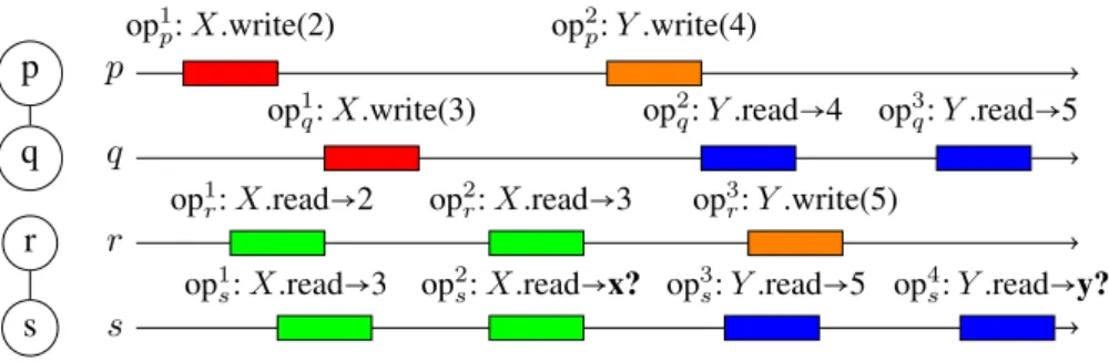
A larger example Figure 6 and Table 1 illustrate the semantic of G-fisheye (SC,CC) consistency on a second, larger, example. In this example, the processes p and q on one hand, and r and s on the other hand, are neighbors in the proximity graphG (shown on the left). There are two pairs of write operations: op1p and op1qon the register X, and op2p and op3ron the register Y . In a sequentially consistency history, both pairs of writes must be seen in the same order by all processes. As a consequence, if r sees the value 2 first (op1r) and then the value 3 (op2r) for X, s must do the same, and only the value 3 can be returned by x?. For the same reason, only the value 3 can be returned by y?, as shown in the first line of Table 1.
In a causally consistent history, however, both pairs of writes ({op1p, op1q} and {op2p, op3r}) are causally independent. As a result, any two processes can see each pair in different orders. x? may return 2 or 3, and y? 4 or 5 (second line of Table 1).
G-fisheye (SC,CC)-consistency provides intermediate guarantees: because p and q are neighbors in G, op1
p and op1q
must be observed in the same order by all processes. x? must return 3, as in a sequentially consistent history. However, because p and r are not connected in G, op2p and op3r may be seen in different orders by different processes (as in a causally consistent history), and y? may return 4 or 5 (last line of Table 1).
p
op1p: X.write(2) op2p: Y .write(4)
q
op1q: X.write(3) op2q: Y .read→4 op3q: Y .read→5
r
op1r: X.read→2 op2r: X.read→3 op3r: Y .write(5)
s
op1
s: X.read→3 op2s: X.read→x? op3s: Y .read→5 op4s: Y .read→y? q
p
r s
Figure 6: IllustratingG-fisheye (SC,CC)-consistency Table 1: Possible executions for the history of Figure 6
Consistency x? y?
Sequential Consistency 3 5
Causal Consistency {2,3} {4,5}
G-fisheye (SC,CC)-consistency 3 {4,5}
4
Construction of an Underlying (SC,CC)-Broadcast Operation
Our implementation ofG-fisheye (SC,CC)-consistency relies on a broadcast operation with hybrid ordering guarantees. In this section, we present this hybrid broadcast abstraction, before moving on the actual implementation of ofG-fisheye (SC,CC)-consistency in Section 5.
4.1 G-fisheye (SC,CC)-broadcast: definition
The hybrid broadcast we proposed, denotedG-(SC,CC)-broadcast, is parametrized by a proximity graph G which deter-mines which kind of delivery order should be applied to which messages, according to the position of the sender in the graphG. Messages (SC,CC)-broadcast by processes which are neighbors in G must be delivered in the same order at all the processes, while the delivery of the other messages only need to respect causal order.
The (SC,CC)-broadcast abstraction provides the processes with two operations, denoted TOCO_broadcast() and TOCO_deliver(). We say that messages are toco-broadcast and toco-delivered.
Causal message order Let M be the set of messages that are toco-broadcast. The causal message delivery order, denoted;M, is defined as follows [10, 33]. Let m1, m2∈ M; m1;M m2, iff one of the following conditions holds:
• m1and m2have been toco-broadcast by the same process, with m1first;
• m1was toco-delivered by a process pibefore this process toco-broadcast m2;
• There exists a message m such that(m1;M m) ∧ (m ;M m2).
Definition of theG-fisheye (SC,CC)-broadcast The (SC,CC)-broadcast abstraction is defined by the following prop-erties.
Validity. If a process toco-delivers a message m, this message was toco-broadcast by some process. (No spurious message.)
Integrity. A message is toco-delivered at most once. (No duplication.)
G-delivery order. For all the processes p and q such that (p, q) is an edge of G, and for all the messages mp and mq
such that mp was toco-broadcast by p and mqwas toco-broadcast by q, if a process toco-delivers mp before mq,
Causal order. If m1 ;M m2, no process toco-delivers m2before m1.
Termination. If a process toco-broadcasts a message m, this message is toco-delivered by all processes.
It is easy to see that ifG has no edges, this definition boils down to causal delivery, and if G is fully connected (clique), this definition specifies total order delivery respecting causal order. Finally, ifG is fully connected and we suppress the “causal order” property, the definition boils to total order delivery.
4.2 G-fisheye (SC,CC)-broadcast: algorithm
Local variables To implement theG-fisheye (SC,CC)-broadcast abstraction, each process pimanages three local
vari-ables.
• causali[1..n] is a local vector clock used to ensure a causal delivery order of the messages; causali[j] is the
sequence number of the next message that piwill toco-deliver from pj.
• totali[1..n] is a vector of logical clock values such that totali[i] is the local logical clock of pi(Lamport’s clock),
and totali[j] is the value of totalj[j] as known by pi.
• pendingi is a set containing the messages received and not yet toco-delivered by pi.
Description of the algorithm Let us remind that for simplicity, we assume that the channels are FIFO. Algorithm 1 describes the behavior of a process pi. This behavior is decomposed into four parts.
The first part (lines 1-6) is the code of the operation TOCO_broadcast(m). Process pifirst increases its local clock
totali[i] and sends the protocol messageTOCOBC(m, ⟨causali[⋅], totali[i], i⟩) to each other process. In addition to the
application message m, this protocol message carries the control information needed to ensure the correct toco-delivery of m, namely, the local causality vector (causali[1..n]), and the value of the local clock (totali[i]). Then, this protocol
message is added to the set pendingiand causali[i] is increased by 1 (this captures the fact that the future application
messages toco-broadcast by piwill causally depend on m).
The second part (lines 7-14) is the code executed by piwhen it receives a protocol messageTOCOBC(m,⟨s causmj [⋅],
s totmj , j⟩) from pj. When this occurs piadds first this protocol message to pendingi, and updates its view of the local
clock of pj (totali[j]) to the sending date of the protocol message (namely, s totmj ). Then, if the local clock of piis late
(totali[i] ≤ s totmj ), pi catches up (line 11), and informs the other processes of it (line 12).
The third part (lines 15-17) is the processing of a catch up message from a process pj. In this case, pi updates its
view of pj’s local clock to the date carried by the catch up message. Let us notice that, as channels are FIFO, a view
stotali[j] can only increase.
The final part (lines 18-31) is a background task executed by pi, where the application messages are toco-delivered.
The set C contains the protocol messages that were received, have not yet been toco-delivered, and are “minimal” with respect to the causality relation ;M. This minimality is determined from the vector clock s causmj [1..n], and the
current value of pi’s vector clock (causali[1..n]). If only causal consistency was considered, the messages in C could
be delivered.
Then, pi extracts from C the messages that can be toco-delivered. Those are usually called stable messages. The
notion of stability refers here to the delivery constraint imposed by the proximity graphG. More precisely, a set T1 is
first computed, which contains the messages of C that (thanks to the FIFO channels and the catch up messages) cannot be made unstable (with respect to the total delivery order defined byG) by messages that pi will receive in the future.
Then the set T2is computed, which is the subset of T1 such that no message received, and not yet toco-delivered, could
make incorrect – w.r.t.G – the toco-delivery of a message of T2.
Once a non-empty set T2has been computed, piextracts the message m whose timestamp⟨s totmj [j], j⟩ is “minimal”
with respect to the timestamp-based total order (pj is the sender of m). This message is then removed from pendingi
and toco-delivered. Finally, if j ≠ i, causali[j] is increased to take into account this toco-delivery (all the messages m′
toco-broadcast by pi in the future will be such that m; m′, and this is encoded in causali[j]). If j = i, this causality
update was done at line 5.
Algorithm 1 TheG-fisheye (SC,CC)-broadcast algorithm executed by pi 1: operationTOCO_broadcast(m)
2: totali[i] ← totali[i] + 1
3: for all pj∈ Π ∖ {pi} do sendTOCOBC(m, ⟨causali[⋅], totali[i], i⟩) to pj 4: pendingi← pendingi∪ ⟨m, ⟨causali[⋅], totali[i], i⟩⟩
5: causali[i] ← causali[i] + 1 6: end operation
7: on receivingTOCOBC(m, ⟨s causmj [⋅], s totmj , j⟩) 8: pendingi← pendingi∪ ⟨m, ⟨s causmj [⋅], s totmj , j⟩⟩
9: totali[j] ← s totmj ▷ Last message from pjhad timestamp s totmj
10: if totali[i] ≤ s totmj then
11: totali[i] ← s totmj + 1 ▷ Ensuring global logical clocks
12: for all pk∈ Π ∖ {pi} do sendCATCH_UP(totali[i], i) to pk 13: end if
14: end on receiving
15: on receivingCATCH_UP(last_datej, j) 16: totali[j] ← last_datej
17: end on receiving
18: background task T is
19: loop forever
20: wait until C≠ ∅ where
21: C≡ {⟨m, ⟨s causmj [⋅], s totmj , j⟩⟩ ∈ pendingi∣ s causmj [⋅] ≤ causali[⋅]} 22: wait until T1≠ ∅ where
23: T1≡ {⟨m, ⟨s causmj [⋅], s totmj , j⟩⟩ ∈ C ∣ ∀pk∈ NG(pj) ∶ ⟨totali[k], k⟩ > ⟨s tot m j , j⟩} 24: wait until T2≠ ∅ where
25: T2≡ ⎧⎪⎪⎪ ⎪⎪⎪ ⎨⎪⎪ ⎪⎪⎪⎪ ⎩ ⟨m, ⟨s causm j [⋅], s totmj , j⟩⟩ ∈ T1 RRRRR RRRRR RRRRR RRRR ∀pk∈ NG(pj), ∀⟨mk,⟨s causmkk[⋅], s totmkk, k⟩⟩ ∈ pendingi∶ ⟨s totmk k , k⟩ > ⟨s tot m j , j⟩ ⎫⎪⎪⎪ ⎪⎪⎪ ⎬⎪⎪ ⎪⎪⎪⎪ ⎭
26: ⟨m0,⟨s causmj00[⋅], s totmj00, j0⟩⟩ ← arg min ⟨m,⟨s causm j [⋅],s tot m j ,j⟩⟩∈T2 {⟨s totm j , j⟩} 27: pendingi← pendingi∖ ⟨m0,⟨s causmj00[⋅], s tot
m j , j0⟩⟩ 28: TOCO_deliver(m0) to application layer
29: if j0≠ i then causali[j0] ← causali[j0] + 1 end if ▷ for causali[i] see line 5 30: end loop forever
4.3 Proof of Theorem 1
The proof combines elements of the proofs of the traditional causal-order [11, 33] and total-order broadcast algo-rithms [22, 7] on which Algorithm 1 is based. It relies in particular on the monoticity of the clocks causali[1..n]
and totali[1..n], and the reliability and FIFO properties of the underlying communication channels. We first prove some
useful lemmata, before proving termination, causal order, and G-delivery order in intermediate theorems. We finally combine these intermediate results to prove Theorem 1.
We use the usual partial order on vector clocks:
C1[⋅] ≤ C2[⋅] iff ∀pi∈ Π ∶ C1[i] ≤ C2[i]
with its accompanying strict partial order:
C1[⋅] < C2[⋅] iff C1[⋅] ≤ C2[⋅] ∧ C1[⋅] ≠ C2[⋅]
We use the lexicographic order on the scalar clocks⟨s totj, j⟩:
⟨s totj, j⟩ < ⟨s toti, i⟩ iff (s totj < s toti) ∨ (s totj = s toti∧ i < j)
We start by three useful lemmata on causali[⋅] and totali[⋅]. These lemmata establish the traditional properties
expected of logical and vector clocks.
Lemma 1 The following holds on the clock values taken by causali[⋅]:
1. The successive values taken bycausali[⋅] in Process piare monotonically increasing.
2. The sequence ofcausali[⋅] values attached toTOCOBCmessages sent out by Processpiare strictly increasing.
Proof Proposition 1 is derived from the fact that the two lines that modify causali[⋅] (lines 5, and 29) only increase
its value. Proposition 2 follows from Proposition 1 and the fact that line 5 insures successiveTOCOBCmessages cannot
include identical causali[i] values. 2Lemma 1
Lemma 2 The following holds on the clock values taken by totali[⋅]:
1. The successive values taken bytotali[i] in Process piare monotonically increasing.
2. The sequence oftotali[i] values included inTOCOBCandCATCH_UPmessages sent out by Processpiare strictly
increasing.
3. The successive values taken bytotali[⋅] in Process piare monotonically increasing.
Proof Proposition 1 is derived from the fact that the lines that modify totali[i] (lines 2 and 11) only increase its value
(in the case of line 11 because of the condition at line 10). Proposition 2 follows from Proposition 1, and the fact that lines 2 and 11 insures successiveTOBOBCandCATCH_UPmessages cannot include identical totali[i] values.
To prove Proposition 3, we first show that:
∀j ≠ i ∶ the successive values taken by totali[j] in piare monotonically increasing. (1)
For j ≠ i, totali[j] can only be modified at lines 9 and 16, by values included inTOBOBCandCATCH_UPmessages,
when these messages are received. Because the underlying channels are FIFO and reliable, Proposition 2 implies that the sequence of last_datej and s totmj values received by pifrom pj is also strictly increasing, which shows equation (1).
From equation (1) and Proposition 1, we conclude that the successive values taken by the vector totali[⋅] in pi are
monotonically increasing (Proposition 3). 2Lemma 2
Lemma 3 Consider an execution of the protocol. The following invariant holds: for i ≠ j, if m is a message sent frompj topi, then at any point ofpi’s execution outside of lines 28-29,s causmj [j] < causali[j] iff that m has been
Proof We first show that if m has been toco-delivered by pi, then s causmj [j] < causali[j], outside of lines 28-29. This
implication follows from the condition s causmj [⋅] ≤ causali[⋅] at line 21, and the increment at line 29.
We prove the reverse implication by induction on the protocol’s execution by process pi. When pi is initialized
causali[⋅] is null:
causal0i[⋅] = [0⋯0] (2)
because the above is true of any process, with Lemma 2, we also have
s causmj [⋅] ≥ [0⋯0] (3)
for all message m that is toco-broadcast by Process pj.
(2) and (3) imply that there are no messages sent by pjso that s causmj [j] < causal0i[j], and the Lemma is thus true
when pistarts.
Let us now assume that the invariant holds at some point of the execution of pi. The only step at which the invariant
might become violated in when causali[j0] is modified for j0≠ i at line 29. When this increment occurs, the condition
s causmj0[j0] < causali[j0] of the lemma potentially becomes true for additional messages. We want to show that there
is only one single additional message, and that this message is m0, the message that has just been delivered at line 28,
thus completing the induction, and proving the lemma. For clarity’s sake, let us denote causal○
i[j0] the value of causali[j0] just before line 29, and causal ●
i[j0] the value
just after. We have causal●
i[j0] = causali○[j0] + 1.
We show that s causm0
j0 [jo] = causal
○
i[j0], where s causmj00[⋅] is the causal timestamp of the message m0delivered
at line 28. Because m0is selected at line 26, this implies that m0∈ T2⊆ T1⊆ C. Because m0∈ C, we have
s causm0
j0 [⋅] ≤ causal
○
i[⋅] (4)
at line 21, and hence
s causm0
j0 [j0] ≤ causal
○
i[j0] (5)
At line 21, m0 has not been yet delivered (otherwise it would not be in pendingi). Using the contrapositive of our
induction hypothesis, we have
s causm0 j0 [j0] ≥ causal ○ i[j0] (6) (5) and (6) yield s causm0 j0 [j0] = causal ○ i[j0] (7)
Because of line 5, m0is the only message tobo_broadcast by Pj0 whose causal timestamp verifies (7). From this
unicity and (7), we conclude that after causali[j0] has been incremented at line 29, if a message m sent by Pj0 verifies
s causmj0[j0] < causali●[j0], then
• either s causmj0[j0] < causali●[j0] − 1 = causal○i[j0], and by induction assumption, m has already been delivered;
• or s causmj0[j0] = causal●i[j0] − 1 < causali○[j0], and m = m0, and m has just been delivered at line 28.
2Lemma 3
Termination
Theorem 2 All messages toco-broadcast using Algorithm 1 are eventually toco-delivered by all processes in the system. Proof We show Termination by contradiction. Assume a process pi toco-broadcasts a message mi with timestamp
⟨s causmi
i [⋅], s tot mi
i , i⟩, and that miis never toco-delivered by pj.
If i≠ j, because the underlying communication channels are reliable, pjreceives at some point theTOCOBCmessage
containing mi(line 7), after which we have
⟨mi,⟨s causmi i[⋅], s totmi i, i⟩⟩ ∈ pendingj (8)
mimight never be toco-delivered by pj because it never meets the condition to be selected into the set C of pj (noted
Cj below) at line 21. We show by contradiction that this is not the case. First, and without loss of generality, we can
choose mi so that it has a minimal causal timestamp s causmi i[⋅] among all the messages that j never toco-delivers (be
it from pi or from any other process). Minimality means here that
∀mx, pjnever delivers mx⇒ ¬(s causmxx < s causmi i) (9)
Let us now assume miis never selected into Cj, i.e., we always have
¬(s causmi
i [⋅] ≤ causalj[⋅]) (10)
This means there is a process pkso that
s causmi
i [k] > causalj[k] (11)
If i= k, we can consider the message m′
isent by i just before mi(which exists since the above implies s caus mi
i [i] >
0). We have s causm′i
i [i] = s caus mi
i [i] − 1, and hence from (11) we have
s causm′i
i [i] ≥ causalj[k] (12)
Applying Lemma 3 to (12) implies that pj never toco-delivers m′i either, with s caus m′i
i [i] < s caus mi
i [i] (by way of
Proposition 2 of Lemma 1), which contradicts (9).
If i ≠ k, applying Lemma 3 to causali[⋅] when pi toco-broadcasts mi at line 3, we find a message mk sent by pk
with s causmk
k [k] = s caus mi
i [k] − 1 such that mkwas received by pibefore pitoco-broadcast mi. In other words, mk
belongs to the causal past of mi, and because of the condition on C (line 21) and the increment at line 29, we have
s causmk
k [⋅] < s caus mi
i [⋅] (13)
As for the case i= k, (11) also implies
s causmk
k [k] ≥ causalj[k] (14)
which with Lemma 3 implies that that pj never delivers the message mkfrom pk, and with (13) contradicts mi’s
mini-mality (9).
We conclude that if a message mi from pi is never toco-delivered by pj, after some point miremains indefinitely in
Cj
mi∈ Cj (15)
Without loss of generality, we can now choose miwith the smallest total order timestamp⟨s totmi i, i⟩ among all the
messages never delivered by pj. Since these timestamps are totally ordered, and no timestamp is allocated twice, there is
only one unique such message.
We first note that because channels are reliable, all processes pk ∈ NG(pi) eventually receive the TOCOBC
proto-col message of pi that contains mi (line 7 and following). Lines 10-11 together with the monotonicity of totalk[k]
(Proposition 1 of Lemma 2), insure that at some point all processes pk have a timestamp totalk[k] strictly larger than
s totmi
i :
∀pk∈ NG(pi) ∶ totalk[k] > s tot mi
i (16)
Since all changes to totalk[k] are systematically rebroadcast to the rest of the system using TOCOBCorCATCHUP
protocol messages (lines 2 and 11), pj will eventually update totalj[k] with a value strictly higher than s totmi i. This
update, together with the monotonicity of totalj[⋅] (Proposition 3 of Lemma 2), implies that after some point:
∀pk∈ NG(pi) ∶ totalj[k] > s tot mi
i (17)
and that mi is selected in T1j. We now show by contradiction that mi eventually progresses to T2j. Let us assume mi
∃pk∈ NG(pi), ∃⟨mk,⟨s caus mk k [⋅], s tot mk k , k⟩⟩ ∈ pendingj ∶ ⟨s totmk k , k⟩ ≤ ⟨s tot m i , i⟩ (18) Note that there could be different pk and mk satisfying (18) in each loop of Task T . However, because NG(pi) is
finite, the number of timestamps⟨s totmk
k , k⟩ such that ⟨s tot mk
k , k⟩ ≤ ⟨s tot m
i , i⟩ is also finite. There is therefore one
process pk0 and one message mk0 that appear infinitely often in the sequence of(pk, mk) that satisfy (18). Since mk0
can only be inserted once into pendingj, this means mk0 remains indefinitely into T
j
2, and hence pendingj, and is never
delivered. (18) and the fact that i≠ k0(because pi/∈ NG(pi)) yields
⟨s totmk0
k , k0⟩ < ⟨s tot m
i , i⟩ (19)
which contradicts our assumption that mihas the smallest total order timestamps⟨s totmi i, i⟩ among all messages never
delivered to pj. We conclude that after some point miremains indefinitely into T2j.
mi∈ T2j (20)
If we now assume miis never returned by arg min at line 26, we can repeat a similar argument on the finite number of
timestamps smaller than⟨s totmi , i⟩, and the fact that once they have been removed form pendingj(line 27), messages are
never inserted back, and find another message mkwith a strictly smaller time-stamp that pj that is never delivered. The
existence of mkcontradicts again our assumption on the minimality of mi’s timestamp⟨s totmi , i⟩ among undelivered
messages.
This shows that miis eventually delivered, and ends our proof by contradiction. 2T heorem 2
Causal Order
We prove the causal order property by induction on the causal order relation;M.
Lemma 4 Consider m1 andm2, two messages toco-broadcast by Processpi, withm1 toco-broadcast before m2. If a
processpjtoco-deliversm2, then it must have toco-deliveredm1beforem2.
Proof We first consider the order in which the messages were inserted into pendingj(along with their causal timestamps
s causmi 1∣2). For i= j, m1was inserted before m2 at line 4 by assumption. For i≠ j, we note that if pj delivers m2 at
line 28, then m2was received from pi at line 7 at some earlier point. Because channels are FIFO, this also means
m1 was received and added to pendingj before m2was. (21)
We now want to show that when m2 is delivered by pj, m1 is no longer in pendingj, which will show that m1 has
been delivered before m2. We use an argument by contradiction. Let us assume that
⟨m1,⟨s causmi 1, s totmi 1, i⟩⟩ ∈ pendingj (22)
at the start of the iteration of Task T which delivers m2to pj. From Proposition 2 of Lemma 1, we have
s causm1
i < s caus m2
i (23)
which implies that m1 is selected into C along with m2(line 21):
⟨m1,⟨s causmi 1, s totmi 1, i⟩⟩ ∈ C
Similarly, from Proposition 2 of Lemma 2 we have: s totm1
i < s tot m2
i (24)
which implies that m1 must also belong to T1 and T2 (lines 23 and 25). (24) further implies that⟨s totmi 2, i⟩ is not the
minimal s tot timestamp of T2, and therefore m0 ≠ m2 in this iteration of Task T . This contradicts our assumption that
m2 was delivered in this iteration; shows that (22) must be false; and therefore with (21) that m1 was delivered before
Lemma 5 Consider m1andm2so thatm1was toco-delivered by a processpibeforepitoco-broadcastsm2. If a process
pj toco-deliversm2, then it must have toco-deliveredm1beforem2.
Proof Let us note pkthe process that has toco-broadcast m1. Because m2is toco-broadcasts by piafter pitoco-delivers
m1 and increments causali[k] at line 29, we have, using Lemma 3 and Proposition 1 of Lemma 1:
s causm1
k [k] < s caus m2
i [k] (25)
Because of the condition on set C at line 21, when pj toco-delivers m2at line 28, we further have
s causm2
i [⋅] ≤ causalj[⋅] (26)
and hence using (25)
s causm1
k [k] < s caus m2
i [k] ≤ causalj[k] (27)
Applying Lemma 3 to (27), we conclude that pjmust have toco-delivered m1 when it delivers m2. 2Lemma 5
Theorem 3 Algorithm 1 respects causal order.
Proof We finish the proof by induction on;M. Let’s consider three messages m1, m2, m3such that
m1;M m3;M m2 (28)
and such that:
• if a process toco-delivers m3, it must have toco-delivered m1;
• if a process toco-delivers m2, it must have toco-delivered m3;
We want to show that if a process toco-delivers m2, it must have tolo-delivered m1. This follows from the transitivity
of temporal order. This result together with Lemmas 4 and 5 concludes the proof. 2T heorem 3
G-delivery order
Theorem 4 Algorithm 1 respectsG-delivery order.
Proof Let’s consider four processes pl, ph, pi, and pj. pland ph are connected inG. plhas toco-broadcast a message
ml, and ph has toco-broadcast a message mh. pi has toco-delivered mlbefore mh. pj has toco-delivered mh. We want
to show that pj has toco-delivered mlbefore mh.
We first show that:
⟨s totmh
h , h⟩ > ⟨s tot ml
l , l⟩ (29)
We do so by considering the iteration of the background task T (lines 18-18) of pi that toco-delivers ml. Because
ph∈ NG(pl), we have
⟨totali[h], h⟩ > ⟨s totml l, l⟩ (30)
at line 23.
If mh has not been received by pi yet, then because of Lemma 3.2, and because communication channels are FIFO
and reliable, we have:
⟨s totmh
h , l⟩ > ⟨totali[h], h⟩ (31)
which with (30) yields (29).
If mhhas already been received by pi, by assumption it has not been toco-delivered yet, and is therefore in pendingi.
More precisely we have:
⟨mh,⟨s causmhh[⋅], s totmhh, h⟩⟩ ∈ pendingi (32)
which, with ph∈ NG(pl), and the fact that mlis selected in T i
We now want to show that pj must have toco-delivered ml before mh. The reasoning is somewhat the symmetric
of what we have done. We consider the iteration of the background task T of pj that toco-delivers mh. By the same
reasoning as above we have
⟨totalj[l], l⟩ > ⟨s totmhh, h⟩ (33)
at line 23.
Because of Lemma 3.2, and because communication channels are FIFO and reliable, (33) and (29) imply that mlhas
already been received by pj. Because mhis selected in T2j at line 25, (29) implies that mhis no longer in pendingj, and
so must have been toco-delivered by pjearlier, which concludes the proof. 2T heorem 4
Theorem 1 Algorithm 1 implements aG-fisheye (SC,CC)-broadcast. Proof
• Validity and Integrity follow from the integrity and validity of the underlying communication channels, and from how a message mjis only inserted once into pendingi (at line 4 if i= j, at line 8 otherwise) and always removed
from pendingiat line 27 before it is toco-delivered by piat line 28;
• G-delivery order follows from Theorem 4; • Causal order follows from Theorem 3; • Termination follows from Theorem 2.
2T heorem 1
5
An Algorithm Implementing
G-Fisheye (SC,CC)-Consistency
5.1 The high level object operations read and write
Algorithm 2 uses theG-fisheye (SC,CC)-broadcast we have just presented to realized G-fisheye (SC,CC)-consistency using a fast-read strategy. This algorithm is derived from the fast-read algorithm for sequential consistency proposed by Attiya and Welch [7], in which the total order broadcast has been replaced by ourG-fisheye (SC,CC)-broadcast.
Algorithm 2 ImplementingG-fisheye (SC,CC)-consistency, executed by pi 1: operation X.write(v)
2: TOCO_broadcast(WRITE(X, v, i)) 3: deliveredi ← false ;
4: wait until deliveredi = true 5: end operation 6: operation X.read() 7: return vx 8: end operation 9: on toco_deliverWRITE(X, v, j) 10: vx← v ;
11: if(i = j) then deliveredi← true endif 12: end on toco_deliver
The write(X, v) operation uses the G-fisheye (SC,CC)-broadcast to propagate the new value of the variable X. To insure any other write operations that must be seen before write(X, v) by piare properly processed, pienters a waiting
loop (line 4), which ends after the message WRITE(X, v, i) that has been toco-broadcast at line 2 is toco-delivered at
line 11.
The read(X) operation simply returns the local copy vx of X. These local copies are updated in the background
Theorem 5 Algorithm 2 implementsG-fisheye (SC,CC)-consistency.
5.2 Proof of Theorem 5
The proof uses the causal order on messages;M provided by theG-fisheye (SC,CC)-broadcast to construct the causal
order on operations ;H. It then gradually extends;H to obtain ★
;H,G. It first uses the property of the broadcast
algorithm on messages to-broadcast by processes that are neighbors inG, and then adapts the technique used in [27, 31] to show that WW (write-write) histories are sequentially consistent. The individual histories ̂Si are obtained by taking a
topological sort of(;★H,G)∣(pi+ W ).
For readability, we denote in the following rp(X, v) the read operation invoked by process p on object X that returns
a value v (X.read→ v), and wp(X, v) the write operation of value v on object X invoked by process p (X.write(v)). We
may omit the name of the process when not needed.
Let us consider a history ̂H= (H,po→H) that captures an execution of Algorithm 2, i.e., po
→H captures the sequence of
operations in each process (process order, po for short). We construct the causal order;H required by the definition of
Section 3.2 in the following, classical, manner:
• We connect each read operation rp(X, v) = X.read → v invoked by process p (with v ≠ , the initial value) to the
write operation w(X, v) = X.write(v) that generated theWRITE(X, v) message carrying the value v to p (line 10
in Algorithm 2). In other words, we add an edge⟨w(X, v)→ rrf p(X, v)⟩ to po
→H (with w and rpas described above)
for each read operation rp(X, v) ∈ H that does not return the initial value . We connect initial read operations
r(X, ) to an element that we add to H.
We call these additional relations read-from links (noted→).rf • We take;H to be the transitive closure of the resulting relation.
;H is acyclic, as assuming otherwise would imply at least one of theWRITE(X, v) messages was received before
it was sent. ;H is therefore an order. We now need to show ;H is a causal order in the sense of the definition of
Section 2.4, i.e., that the result of each read operation r(X, v) is the value of the latest write w(X, v) that occurred before r(X, v) in ;H (said differently, that no read returns an overwritten value).
Lemma 6 ;H is a causal order.
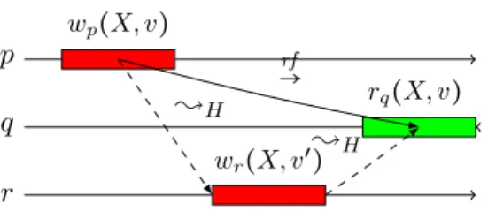
Proof We show this by contradiction. We assume without loss of generality that all values written are distinct. Let us consider wp(X, v) and rq(X, v) so that wp(X, v)
rf
→ rq(X, v), which implies wp(X, v) ;H rq(X, v). Let us assume
there exists a second write operation wr(X, v′) ≠ wp(X, v) on the same object, so that
wp(X, v) ;H wr(X, v′) ;H rq(X, v) (34)
(illustrated in Figure 7). wp(X, v) ;H wr(X, v′) means we can find a sequence of operations opi∈ H so that
wp(X, v) →0op0...→iopi→i+1...→kwr(X, v′) (35)
with →i∈ { po
→H, rf
→}, ∀i ∈ [1, k]. The semantics of po→H and rf
→ means we can construct a sequence of causally related (SC,CC)-broadcast messages mi ∈ M between the messages that are toco-broadcast by the operations wp(X, v) and
wr(X, v′), which we noteWRITEp(X, v) andWRITEr(X, v′) respectively:
WRITEp(X, v) = m0 ;M m1...;M mi;M ...;M mk′=WRITEr(X, v′) (36)
where;M is the message causal order introduced in Section 4.1. We conclude thatWRITEp(X, v) ;M WRITEr(X, v′),
i.e., that WRITEp(X, v) belongs to the causal past of WRITEr(X, v′), and hence that q in Figure 7 toco-delivers WRITEr(X, v′) afterWRITEp(X, v).
We now want to show thatWRITEr(X, v′) is toco-delivered by q before q executes rq(X, v). We can apply the same
reasoning as above to wr(X, v′) ;H rq(X, v), yielding another sequence of operations op′i∈ H:
wr(X, v′) →′0op ′ 0...→ ′ iop ′ i→ ′ i+1...→ ′ k′′ rq(X, v) (37)
p wp(X, v) q rq(X, v) r wr(X, v′) rf → ;H ;H
Figure 7: Proving that;H is causal by contradiction
with→′ i∈ {
po
→H, rf
→}. Because rq(X, v) does not generate any (SC,CC)-broadcast message, we need to distinguish the case
where all op′
i relations correspond to the process order po
→H (i.e., op′i = po
→H,∀i). In this case, r = q, and the blocking
be-havior of X.write() (line 4 of Algorithm 2), insures thatWRITEr(X, v′) is toco-delivered by q before executing rq(X, v).
If at least one op′
icorresponds to the read-from relation, we can consider the latest one in the sequence, which will denote
the toco-delivery of aWRITEz(Y, w) message by q, withWRITEr(X, v′) ;M WRITEz(Y, w). From the causality of the
(SC,CC)-broadcast, we also conclude thatWRITEr(X, v′) is toco-delivered by q before executing rq(X, v).
Because q toco-delivers WRITEp(X, v) beforeWRITEr(X, v′), and toco-deliversWRITEr(X, v′) before it executes
rq(X, v), we conclude that the value v of vx is overwritten by v′at line 10 of Algorithm 2, and that rq(X, v) does not
return v, contradicting our assumption that wp(X, v) rf
→ rq(X, v), and concluding our proof that ;H is a causal order.
2Lemma 6
To construct;★H,G, as required by the definition of (SC,CC)-consistency (Section 3.2), we need to order the write
operations of neighboring processes in the proximity graphG. We do so as follows: • We add an edge wp(X, v)
ww
→ wq(Y, w) to ;H for each pair of write operations wp(X, v) and wq(Y, w) in H
such that:
– (p, q) ∈ EG(i.e., p and q are connected inG);
– wp(X, v) and wq(Y, w) are not ordered in ;H;
– The broadcast message WRITEp(X, v) of wp(X, v) has been toco-delivered before the broadcast message WRITEp(Y, w) of wq(Y, w) by all processes.
We call these additional edges ww links (notedww→ ).
• We take;★H,Gto be the recursive closure of the relation we obtain. ★
;H,G is acyclic, as assuming otherwise would imply that the underlying (SC,CC)-broadcast violates causality.
Be-cause of theG-delivery order and termination of the toco-broadcast (Section 4.1), we know all pairs ofWRITEp(X, v)
andWRITEp(Y, w) messages with (p, q) ∈ EG as defined above are toco-delivered in the same order by all processes.
This insures that all write operations of neighboring processes inG are ordered in;★H,G.
We need to show that;★H,Gremains a causal order, i.e., that no read in ★
;H,Greturns an overwritten value.
Lemma 7 ;★H,G is a causal order.
Proof We extend the original causal order;M on the messages of an (SC,CC)-broadcast execution with the following
order;G M:
m1 ;GM m2if
• m1;M m2; or
• m1was sent by p, m2by q,(p, q) ∈ EG, and m1 is toco-delivered before m2by all processes; or
;G
M captures the order imposed by an execution of an (SC,CC)-broadcast on its messages. The proof is then identical to
that of Lemma 6, except that we use the order;G
M, instead of;M. 2Lemma 7
Theorem 5 Algorithm 2 implementsG-fisheye (SC,CC)-consistency.
Proof The order;★H,G we have just constructed fulfills the conditions required by the definition ofG-fisheye
(SC,CC)-consistency (Section 3.2):
• by construction;★H,Gsubsumes;H (;H ⊆ ★
;H,G);
• also by construction ;★H,G, any pair of write operations invoked by processes p,q that are neighbors in G are
ordered in;★H,G; i.e.,( ★
;H,G)∣({p, q} ∩ W ) is a total order.
To finish the proof, we choose, for each process pi, ̂Sias one of the topological sorts of( ★
;H,G)∣(pi+ W ), following
the approach of [27, 31]. ̂Si is sequential by construction. Because ★
;H,G is causal, ̂Siis legal. Because ★
;H,G respects po
→H, ̂Siis equivalent to ̂H∣(pi+ W ). Finally, ̂Sirespects( ★
;H,G)∣(pi+ W ) by construction. 2T heorem 5
6
Conclusion
This work was motivated by the increasing popularity of geographically distributed systems. We have presented a frame-work that enables to formally define and reason about mixed consistency conditions in which the operations invoked by nearby processes obey stronger consistency requirements than operations invoked by remote ones. The framework is based on the concept of a proximity graph, which captures the “closeness” relationship between processes. As an ex-ample, we have formally definedG-fisheye (SC,CC)-consistency, which combines sequential consistency for operations by close processes with causal consistency among all operations. We have also provided a formally proven protocol for implementingG-fisheye (SC,CC)-consistency.
Another natural example that has been omitted from this paper for brevity isG-fisheye (LIN,SC)-consistency, which combines linearizability for operations by nearby nodes with an overall sequential consistency guarantee.
The significance of our approach is that the definitions of consistency conditions are functional rather than opera-tional. That is, they are independent of a specific implementation, and provide a clear rigorous understanding of the provided semantics. This clear understanding and formal underpinning comes with improved complexity and perfor-mance, as illustrated in our implementation ofG-fisheye (SC,CC)-consistency, in which operations can terminate without waiting to synchronize with remote parts of the system.
More generally, we expect the general philosophy we have presented to extend to Convergent Replicated Datatypes (CRDT) in which not all operations are commutative [28]. These CRDTs usually require at a minimum causal commu-nications to implement eventual consistency. The hybridization we have proposed opens up the path of CRDTs which are globally eventually consistent, and locally sequentially consistent, a route we plan to explore in future work.
Acknowledgments
This work has been partially supported by a French government support granted to the CominLabs excellence laboratory (Project DeSceNt: Plug-based Decentralized Social Network) and managed by the French National Agency for Research (ANR) in the "Investing for the Future" program under reference Nb. ANR-10-LABX-07-01, and by the SocioPlug Project funded by French National Agency for Research (ANR), under program ANR INFRA (ANRANR-13-INFR-0003). We would also like to thank Matthieu Perrin for many enlightening discussions on the topic of weak consistency models, and for pointing out a flaw in an earlier definition of fisheye consistency.
References
[2] Ahamad M., Niger G., Burns J.E., Hut to P.W., and Kohl P. Causal memory: definitions, implementation and programming. Dist. Computing, 9:37-49, 1995.
[3] Almeida S., Leitaõ J., Rodrigues L., ChainReaction: a Causal+ Consistent Datastore based on Chain Replication. 8th ACM Europ. Conf. on Comp. Sys. (EuroSys’13), pp. 85-98, 2013.
[4] Alvaro P., Bailis P., Conway N., and Hellerstein J. M. Consistency without borders 4th ACM Symp. on Cloud Computing (SOCC ’13), 2013, 23
[5] Attiya H. and Friedman R., A correctness condition for high-performance multiprocessors. SIAM Journal on Computing, 27(6):1637-1670, 1998.
[6] Attiya H. and Friedman R., Limitations of Fast Consistency Conditions for Distributed Shared Memories. Information Pro-cessing Letters, 57(5):243-248, 1996.
[7] Attiya H. and Welch J.L., Sequential consistency versus linearizability. ACM Trans. on Comp. Sys., 12(2):91-12, 1994. [8] Attiya H. and Welch J.L., Distributed computing: fundamentals, simulations and advanced topics, (2nd Edition), Wiley-Inter
science, 414 pages, 2004 (ISBN 0-471-45324-2).
[9] Bailis P., Ghodsi A., Hellerstein J. M., and Stoica I., Bolt-on Causal Consistency 2013 ACM SIGMOD Int. Conf. on Manage-ment of Data (SIGMOD’13), pp. 761-772, 2013.
[10] Birman K.P. and Joseph T.A., Reliable communication in presence of failures. ACM Trans. on Comp. Sys., 5(1):47-76, 1987. [11] Birman K., Schiper A., and Stephenson P., Lightweight Causal and Atomic Group Multicast ACM Trans. Comput. Syst., vol.
9, pp. 272-314, 1991.
[12] Brewer E., Towards Robust Towards Robust Distributed Systems 19th ACM Symposium on Principles of Distributed Comput-ing (PODC), Invited talk, 2000.
[13] Burckhardt S., Gotsman A., Yang H., and Zawirski M., Replicated Data Types: Specification, Verification, Optimality 41st ACM Symp. on Principles of Prog. Lang. (POPL’14), pp. 271-284, 2014.
[14] DeCandia G., Hastorun D., Jampani M., Kakulapati G., Lakshman A., Pilchin A., Sivasubramanian S., Vosshall P., and Vogels W., Dynamo: amazon’s highly available key-value store 21st ACM Symp. on Op. Sys. Principles (SOSP’07), pp. 205-220, 2007 [15] Friedman R., Implementing Hybrid Consistency with High-Level Synchronization Operations. Distributed Computing,
9(3):119-129, 1995.
[16] Garg V.K. and Raynal M., Normality: a consistency condition for concurrent objects. Parallel Processing Letters, 9(1):123-134, 1999.
[17] , Gharachorloo K., Lenoski D., Laudon J., Gibbons P., Gupta A., and Hennessy J., Memory consistency and event ordering in scalable shared-memory multiprocessors. 17th ACM Annual International Symp. on Comp. Arch. (ISCA), pp. 15-26, 1990. [18] Herlihy M. and and Shavit N., The Art of Multiprocessor Programming, Morgan Kaufmann Publishers Inc., 508 pages, 2008
(ISBN 978-0-12-370591-4).
[19] Herlihy M. and Wing J., Linearizability: a correctness condition for concurrent objects. ACM Transactions on Programming Languages and Systems, 12(3):463–492, 1990.
[20] Keleher P. Cox A.L., and Zwaenepoel W., Lazy release consistency for software distributed shared memory. Proc. 19th ACM Int’l Symp. on Comp. Arch. (ISCA’92), pages 13–21, 1992.
[21] Lakshman A., and Malik P., Cassandra: a decentralized structured storage system. SIGOPS Oper. Syst. Rev., volume 44, pp. 35-40, 201.
[22] Lamport L., Time, Clocks and the Ordering of Events in a Distributed System Comm. of the ACM, vol. 21, pp. 558-565, 1978 [23] Lamport L., How to make a multiprocessor computer that correctly executes multiprocess programs. IEEE Trans. on Comp.,
C28(9):690–691, 1979.
[25] Lloyd W., Freedman M. J., Kaminsky M., and Andersen D. G., Don’t Settle for Eventual: Scalable Causal Consistency for Wide-area Storage with COPS 23rd ACM Symp. on Op. Sys. Principles, pp. 401-416, 2011
[26] Lynch N.A., Distributed Algorithms. Morgan Kaufman Pub., San Francisco (CA), 872 pages, 1996.
[27] Mizuno M., Raynal M., and Zhou J. Z., Sequential Consistency in Distributed Systems Selected Papers from the International Workshop on Theory and Practice in Dist. Sys., Springer, pp. 224-241, 1995
[28] Oster, G., Urso, P., Molli, P., and Imine, A. Data consistency for P2P collaborative editing. Proceedings of the 2006 20th anniversary conference on Computer supported cooperative work, ACM, pp. 259-268, 2006
[29] Preguiça N.M., Marquès, J.M., Shapiro M., and Letia M., A Commutative Replicated Data Type for Cooperative Editing. Proc. 29th IEEE Int’l Conf. on Dist. Comp. Sys. (ICDCS’09), pp. 395–403, 2009.
[30] Raynal M., Concurrent Programming: Algorithms, Principles, and Foundations, Springer, 515 pages, 2013, ISBN 978-3-642-32026-2.
[31] Raynal M., Distributed Algorirhms for Message-passing Systems, Springer, 500 pages, 2013, ISBN 978-3-642-38122-5. [32] Raynal M. and Schiper A., A suite of formal definitions for consistency criteria in distributed shared Memories. 9th Int’l IEEE
Conf. on Parallel and Dist. Comp. Sys. (PDCS’96), pp. 125-131, 1996.
[33] Raynal M., Schiper A., and Toueg S., The Causal Ordering Abstraction and a Simple Way to Implement. Information Process-ing Letters, 39(6):343-350, 1991.
[34] Saito Y. and Shapiro M., Optimistic Replication. it ACM Computing Survey, 37(1):42-81, March 2005.
[35] Shapiro M., Preguiça N.M., Baquero C., and Zawirski M., Convergent and Commutative Replicated Data Types. Bulletin of the EATCS, 104:67-88, 2011.
[36] Sovran Y., Power R., Aguilera M. K., and Li J., Transactional Storage for Geo-Replicated Systems. 23rd ACM Symposium on Operating Systems Principles (SOSP’11), pp. 385-400, 2011.
[37] Terry D. B., Prabhakaran V., Kotla R., Balakrishnan M., Aguilera M. K., and Abu-Libdeh H., Consistency-based Service Level Agreements for Cloud Storage, 24th ACM Symp. on Op. Sys. Principles (SOSP’13), pp. 309-324, 2013.
[38] Terry D. B., Theimer M. M., Petersen K., Demers A. J., Spreitzer M. J., and Hauser C. H., Managing Update Conflicts in Bayou, a Weakly Connected Replicated Storage System 15th ACM Symp. on Op. Sys. Principles (SOSP’95), pp. 172-182, 1995.
[39] Xie C., Su C., Kapritsos M., Wang Y., Yaghmazadeh N., Alvisi L., and Mahajan P., Salt: Combining ACID and BASE in a Distributed Database. USENIX Operating Systems Design and Implementation (OSDI), 2014.