DOCTORAT DE L'UNIVERSITÉ DE TOULOUSE
Délivré par :
Institut National Polytechnique de Toulouse (INP Toulouse)
Discipline ou spécialité :
Signal, Image, Acoustique et Optimisation
Présentée et soutenue par :
M. QI WEI
le jeudi 24 septembre 2015
Titre :
Unité de recherche :
Ecole doctorale :
BAYESIAN FUSION OF MULTI-BAND IMAGES: A POWERFUL TOOL
FOR SUPER-RESOLUTION
Mathématiques, Informatique, Télécommunications de Toulouse (MITT)
Institut de Recherche en Informatique de Toulouse (I.R.I.T.)
Directeur(s) de Thèse :
M. JEAN YVES TOURNERETM. NICOLAS DOBIGEON
Rapporteurs :
M. CÉDRIC RICHARD, UNIVERSITE DE NICE SOPHIA ANTIPOLIS M. PAUL SCHEUNDERS, UNIVERSITE INSTELLING ANTWERPEN
Membre(s) du jury :
1 M. XAVIER BRIOTTET, ONERA TOULOUSE, Président
2 M. JEAN YVES TOURNERET, INP TOULOUSE, Membre
2 M. JOSE BIOUCAS-DIAS, INSTITUTO SUPERIOR TECNICO LISBONNE, Membre
2 Mme GWENDOLINE BLANCHET, CENTRE NATIONAL D'ETUDES SPATIALES CNES, Membre
I would like to express my special appreciation and thanks to my supervisor professor Jean-Yves Tourneret, you have been a tremendous mentor for me. I would like to thank you for encouraging my research and for allowing me to grow as a problem solver. You have brought the magic of Bayesian inference to me and let me feel the power of MCMC when processing non-convex problems. Thank you very much for supporting me to visit professor José Bioucas-Dias and sending me several times to different conferences, which in fact helps a lot for my work. Besides, your advice on both research as well as on my career have been priceless.
I would also like to thank my co-supervisor Nicolas Dobigeon. You have given me numerous guidances, both theoretically and practically. Without your help, a lot of works would have not been finished smoothly. You have taught me many tricks of coding and writing, which accelerates my progress much. You are always patient and helps me in many details, such as latex writing skills, reference management, etc. Besides, thank you for helping me process the TWINGO surprise.
Especially, I would like to give my many thanks to professor José Bioucas-Dias, who opens the door of optimization for me, making me aware of such a flourish field. You have taught me a lot of op-timization techniques, such as ADMM, dictionary learning, sparse coding, proximity operations, etc. Your insightful analysis for inverse problems in image processing as well as our profound discussion have enlightened me and broadened my horizon greatly.
I would like to thank China Scholarship Council (CSC) for supporting my PhD at University of Toulouse. I would also like to thank my committee members, professor Christophe Collet, professor Cédric Richard, professor Paul Scheunders, professor José Bioucas-Dias (again), professor Xavier
lot from your insightful reviews, comments, remarks and questions about my work.
I am very grateful to professor Simon Godsill at University of Cambridge and professor Michael Elad at Technion, who supported my visiting to their groups, where I have seen very impressive works from excellent students and professors.
I would like to thank Rob Heylen, Émilie Chouzenoux, Saïd Moussaoui, Yifan Zhang, Paul Scheunders (again) for sharing the codes of their works and Jordi Inglada, from Centre National d’Études Spatiales (CNES), for providing the LANDSAT spectral responses used in my works. I am also grateful to Nathalie Brun for sharing the EELS data and offering useful suggestions to process them. I thank Frank Deutsch for helpful discussion on the convergence rate of the alternating projections.
I want to thank the other professors in the IRIT-SC group, including Benoit, Charly, Corinne, Hasan, Herwig, Marie, Marie-Laure, Martial, Nathalie · · · I would also like to thank my colleagues from office F423 who have accompanied me in the pasting three years: Abder, Cécile, Matthieu, Ningning, Pierre-Antoine, Sébastien and Yoann, and my friends: Alexandre, Bouchra, Feng, Jean-Adrien, Jorge, Oliver, Qiankun, Raoul, Romain, Tao, Tarik, Tony, Sokchenda, Victor · · · Besides, I would give my great thanks to Sylvie Eichen, Sylvie Armengaud and Audrey Cathala, who have been our very efficient sectaries in IRIT-ENSEEIHT.
A special thanks to my family. Words cannot express how grateful I am to my mother, father, brother and sister-in-law for all of the sacrifices that you have made on my behalf. Your prayer for me was what sustained me thus far. A special thanks is given to my girlfriend Ningning. You have accompanied me for long time and helped me overcome many difficulties, both in research and in life. You are always my support in the moments when there was no one to answer my queries.
Qi WEI
Hyperspectral (HS) imaging, which consists of acquiring a same scene in several hundreds of contigu-ous spectral bands (a three dimensional data cube), has opened a new range of relevant applications, such as target detection [MS02], classification [C.-03] and spectral unmixing [BDPD+12]. However,
while HS sensors provide abundant spectral information, their spatial resolution is generally more limited. Thus, fusing the HS image with other highly resolved images of the same scene, such as multispectral (MS) or panchromatic (PAN) images is an interesting problem. The problem of fus-ing a high spectral and low spatial resolution image with an auxiliary image of higher spatial but lower spectral resolution, also known as multi-resolution image fusion, has been explored for many years [AMV+11]. From an application point of view, this problem is also important as motivated by
recent national programs, e.g., the Japanese next-generation space-borne hyperspectral image suite (HISUI), which fuses co-registered MS and HS images acquired over the same scene under the same conditions [YI13]. Bayesian fusion allows for an intuitive interpretation of the fusion process via the posterior distribution. Since the fusion problem is usually ill-posed, the Bayesian methodology offers a convenient way to regularize the problem by defining appropriate prior distribution for the scene of interest.
The aim of this thesis is to study new multi-band image fusion algorithms to enhance the resolu-tion of HS image. In the first chapter, a hierarchical Bayesian framework is proposed for multi-band image fusion by incorporating forward model, statistical assumptions and Gaussian prior for the target image to be restored. To derive Bayesian estimators associated with the resulting posterior distribution, two algorithms based on Monte Carlo sampling and optimization strategy have been
served images is introduced as an alternative of the naive Gaussian prior proposed in Chapter 1 to regularize the ill-posed problem. Identifying the supports jointly with the dictionaries circumvented the difficulty inherent to sparse coding. To minimize the target function, an alternate optimization algorithm has been designed, which accelerates the fusion process magnificently comparing with the simulation-based method. In the third chapter, by exploiting intrinsic properties of the blurring and downsampling matrices, a much more efficient fusion method is proposed thanks to a closed-form solution for the Sylvester matrix equation associated with maximizing the likelihood. The proposed solution can be embedded into an alternating direction method of multipliers or a block coordinate descent method to incorporate different priors or hyper-priors for the fusion problem, allowing for Bayesian estimators. In the last chapter, a joint multi-band image fusion and unmixing scheme is proposed by combining the well admitted linear spectral mixture model and the forward model. The joint fusion and unmixing problem is solved in an alternating optimization framework, mainly consisting of solving a Sylvester equation and projecting onto a simplex resulting from the non-negativity and sum-to-one constraints. The simulation results conducted on synthetic and semi-synthetic images illustrate the advantages of the developed Bayesian estimators, both qualitatively and quantitatively.
Acronymes
ADMM alternating direction method of multipliers ANC abundance non-negativity constraint ASC abundance sum-to-one constraint
AVIRIS airborne visible/infrared imaging spectrometer BCD block coordinate descent
BNNT boron-nitride nanotubes
CNMF coupled nonnegative matrix factorization C-SUnSAL constrained SUnSAL
CSC China Scholarship Council DAG directed acyclic graph DD degree of distortion DFT discrete Fourier transform DL dictionary learning
DLR Deutsches Zentrum für Luft- und Raumfahrt, the German Aerospace Agency DR dimensionality reduction
EEA endmember extraction algorithm EELS electron energy-loss spectroscopy
FUMI fusion and unmixing of multi-band images FUSE Fast fUsion based on Sylvester Equation GPU graphics processing units
HISUI hyperspectral imager suite HMC Hamiltonian Monte Carlo HS hyperspectral
HySime hyperspectral signal subspace identification by minimum error ICA independent component analysis
IGMRF in-homogeneous Gaussian Markov random field i.i.d independent and identically distributed
IRIT Institut de Recherche en Informatique de Toulouse KKT Karush-Kuhn-Tucker
LASSO last absolute shrinkage and selection operator LIP linear inverse problem
LLE locally linear embedding LMM linear mixing model LS least-square
MAP maximum a posteriori MCMC Markov Chain Monte Carlo MCRD minimum change rate deviation
METI ministry of economy, trade, and industry MMSE minimum mean square error
MS multispectral
NCLS non-negativity constrained least squares NMSE normalized mean square error
ODL online dictionary learning OMP orthogonal matching pursuit PAN Panchromatic image
PCA principal component analysis PDF probability density function POCS projections onto convex sets RMSE root mean square error
ROSIS reflective optics system imaging spectrometer RSNR reconstruction SNR
SALSA split augmented Lagrangian shrinkage algorithm SAM spectral angle mapper
SE Sylvester equation SNR signal to noise ratio SU Spectral unmixing
SUnSAL sparse unmixing algorithm by variable splitting and augmented Lagrangian SVMAX successive volume maximization
TV total variation
VCA vertex component analysis w.r.t. with respect to
UIQI universal image quality index
≪ much lower ≫ much greater
δ(·) Dirac delta function ⊗ Kronecker product ë · ëF Frobenius norm ë · ë2 ℓ2 norm ë · ë1 ℓ1 norm ë · ë0 ℓ0 pseudo norm tr (·) trace of matrix xi
X target image
xi ith column of X
U target image in a subspace ui ith column of U
H lower dimensional subspace transformation matrix ·T transpose operator YH observed HS image YM observed MS image NH HS noise NM MS noise B blurring matrix S downsampling matrix R spectral response E endmember matrix A abundance matrix xii
mc column number of the HS image
mλ band number of the HS image
m number of pixels in each band of the HS image, i.e., m = mr× mc
nr row number of the MS image
nc column number of the MS image
nλ band number of the MS image
n number of pixels in each band of the MS image, i.e., n = nr× nc
dr decimation factor in row
dc decimation factor in column
d decimation factor in two-dimension, i.e., d = dr× dc
å
mλ dimension of subspace
Usual distributions
MN (M, Σr, Σc) matrix normal distribution with mean M, row covariance matrix Σr and column covariance matrix Σc
IG!ν2,
γ
2
" inverse-gamma distribution with shape parameter ν and scale parameter γ
IW(Ψ, η) inverse-Wishart distribution with shape parameter Ψ and scale parameter η
Acknowledgements iii
Abstract v
Acronyms and notations viii
Introduction 1
List of publications 13
Chapter 1 Bayesian fusion of multi-band images using a Gaussian prior 17
1.1 Introduction . . . 18
1.1.1 Bayesian estimation of X . . . 19
1.1.2 Lower-dimensional subspace . . . 20
1.1.3 Likelihood and prior distributions . . . 21
1.1.4 Hyperparameter prior . . . 22
1.1.5 Posterior distribution . . . 22
1.1.6 Inferring the highly-resolved HS image from the posterior of U . . . 23
1.1.7 Hybrid Gibbs sampler . . . 24
1.1.8 Complexity analysis . . . 28
1.2 Simulation results (MCMC algorithm) . . . 28
1.2.1 Fusion of HS and MS images . . . 28
1.2.3 Evaluation of the fusion quality . . . 32
1.2.4 Comparison with other Bayesian models . . . 34
1.2.5 Estimation of the noise variances . . . 35
1.2.6 Robustness with respect to the knowledge of R . . . 35
1.2.7 Application to Pansharpening . . . 36
1.3 Block Coordinate Descent method . . . 38
1.3.1 Optimization with respect to U . . . 39
1.3.2 Optimization with respect to s2 . . . 40
1.3.3 Optimization with respect to Σ . . . 41
1.3.4 Relationship with the MCMC method . . . 42
1.4 Simulation results (BCD algorithm) . . . 42
1.4.1 Simulation scenario . . . 42
1.4.2 Hyperparameter selection . . . 44
1.4.3 Fusion performance . . . 44
1.5 Conclusion . . . 46
Chapter 2 Bayesian fusion based on a sparse representation 47 2.1 Introduction . . . 48
2.2 Problem formulation . . . 49
2.2.1 Notations and observation model . . . 49
2.2.2 Subspace learning . . . 50
2.3 Proposed fusion method for MS and HS images . . . 50
2.3.1 Ill-posed inverse problem . . . 50
2.3.2 Sparse regularization . . . 52
2.3.3 Dictionary learning . . . 53
2.3.4 Including the sparse code into the estimation framework . . . 54
2.4 Alternate optimization . . . 55
2.4.3 Complexity analysis . . . 59
2.5 Simulation results on synthetic data . . . 59
2.5.1 Simulation scenario . . . 60
2.5.2 Learning the subspace, the dictionaries and the code supports . . . 61
2.5.3 Comparison with other fusion methods . . . 63
2.5.4 Selection of the regularization parameter λ . . . 66
2.5.5 Test with other datasets . . . 67
2.6 Conclusions . . . 73
Chapter 3 Fast fusion based on solving a Sylvester equation 75 3.1 Introduction . . . 76
3.1.1 Background . . . 76
3.1.2 Problem statement . . . 76
3.1.3 Chapter organization . . . 78
3.2 Problem formulation . . . 78
3.3 Fast fusion scheme . . . 80
3.3.1 Sylvester equation . . . 80
3.3.2 Existence of a solution . . . 81
3.3.3 A classical algorithm for the Sylvester matrix equation . . . 82
3.3.4 Proposed closed-form solution . . . 82
3.3.5 Complexity analysis . . . 85
3.4 Generalization to Bayesian estimators . . . 86
3.4.1 Gaussian prior . . . 87
3.4.2 Non-Gaussian prior . . . 88
3.4.3 Hierarchical Bayesian framework . . . 91
3.5 Experimental results . . . 92
3.5.2 Hyperspectral Pansharpening . . . 98
3.6 Conclusion . . . 103
Chapter 4 Multi-band image fusion based on spectral unmixing 105 4.1 Introduction . . . 105
4.2 Problem Statement . . . 107
4.2.1 Linear Mixture Model . . . 107
4.2.2 Forward model . . . 108
4.2.3 Composite fusion model . . . 109
4.2.4 Statistical methods . . . 109
4.3 Problem Formulation . . . 110
4.3.1 Data fitting terms (likelihoods) . . . 110
4.3.2 Constraints and regularizations (priors) . . . 111
4.3.3 Constrained optimization formulation . . . 112
4.4 Alternating Optimization Scheme . . . 113
4.4.1 Optimization w.r.t. the abundance matrix A . . . 113
4.4.2 Optimization w.r.t. the endmember matrix M . . . 116
4.4.3 Convergence analysis . . . 119 4.5 Experimental results . . . 120 4.5.1 Quality metrics . . . 120 4.5.2 Synthetic data . . . 121 4.5.3 Semi-real data . . . 124 4.6 Conclusion . . . 128
Conclusions and perspectives 137 4.6.1 Conclusion . . . 137
4.6.2 Future work . . . 139
A.1 Problem formulation . . . 145
A.1.1 Notations and observation model . . . 145
A.1.2 Bayesian estimation of x . . . 146
A.2 Hierarchical Bayesian model . . . 147
A.2.1 Likelihood function . . . 147
A.2.2 Prior distributions . . . 148
A.2.3 Hyperparameter priors . . . 150
A.2.4 Inferring the highly-resolved HS image from the posterior distribution of its projection u . . . 152
A.3 Hybrid Gibbs Sampler . . . 153
A.3.1 Sampling Σ according to f!Σ|u, s2, z" . . . 153
A.3.2 Sampling u according to f!u|Σ, s2, z" . . . 154
A.3.3 Sampling s2 according to f!s2|u, Σ, z" . . . 156
Appendix B Fusion with unknown spectral response R . . . 157
B.1 Problem formulation . . . 157
B.2 Hierarchical Bayesian model . . . 157
B.2.1 Reformulation in a lower-dimensional subspace . . . 157
B.2.2 Likelihood and prior distributions . . . 158
B.2.3 Hyperparameter priors . . . 159
B.2.4 Posterior distribution . . . 159
B.3 Hybrid Gibbs sampler . . . 160
B.3.1 Sampling the covariance matrix of the image Σ . . . 160
B.3.2 Sampling the pseudo-spectral response matrix Rå . . . 160
B.3.3 Sampling the projected image U . . . 161
B.3.4 Sampling the noise variance vector s2 . . . 161
B.4 Simulation results . . . 162
B.4.2 Hyperparameter Selection . . . 163
B.4.3 Fusion performance . . . 163
B.5 Conclusion . . . 167
Appendix C Proofs related to FUSE algorithm . . . 169
C.1 Proof of Lemma 1 . . . 169
C.2 Proof of Lemma 2 . . . 169
C.3 Proof of Lemma 3 . . . 171
C.4 Proof of Theorem 1 . . . 172
Appendix D A fast unmixing algorithm SUDAP . . . 175
Bibliography 207
1 Hyperspectral data cube . . . 2 2 (Left) Hyperspectral image (size: 99 × 46 × 224, res.: 80m × 80m). (Middle)
Panchro-matic image (size: 396 × 184 res.: 20m × 20m). (Right) Target image (size: 396 × 184× 224 res.: 20m × 20m). . . 3 1.1 LANDSAT-like spectral responses. . . 29 1.2 AVIRIS dataset: (Top 1) HS image. (Top 2) MS image. (Top 3) Reference image.
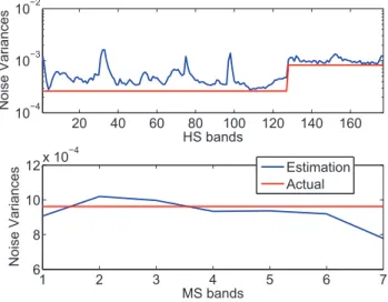
(Middle 1) MAP [HEW04]. (Middle 2) Wavelet MAP [ZDBS09]. (Middle 3) MCMC. (Bottom 1-3) The corresponding RMSE errors. . . 30 1.3 Eigenvalues of Υ for the HS image. . . 30 1.4 Noise variances and their MMSE estimates. (Top) HS image. (Bottom) MS image. . . 35 1.5 LANDSAT-like spectral responses. (Top) without noise. (Bottom) with an additive
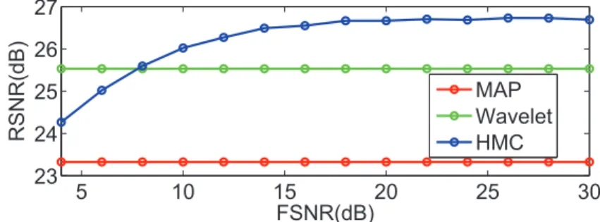
Gaussian noise with FSNR = 8dB. . . 36 1.6 Reconstruction errors of the different fusion methods versus FSNR. . . 37 1.7 ROSIS dataset: (Top left) Reference image. (Top right) PAN image. (Middle left)
Adaptive IHS [RSM+10]. (Middle right) MAP [HEW04]. (Bottom left) Wavelet MAP
[ZDBS09]. (Bottom right) MCMC. . . 38 1.8 AVIRIS dataset: (Top 1) HS image. (Top 2) MS image. (Top 3) Reference image.
(Middle 1) MAP [HEW04]. (Middle 2) Wavelet MAP [ZDBS09]. (Middle 3) MCMC. (Middle 4): Proposed method. (Bottom 1-4) The corresponding RMSE maps (more black, smaller errors; more white, larger errors). . . 43
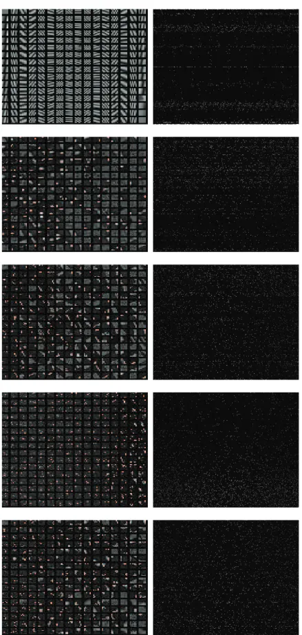
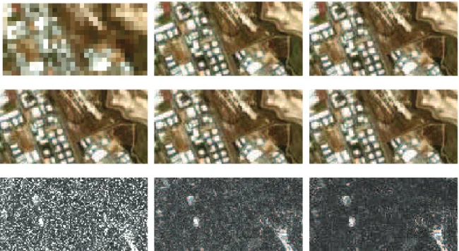
2.1 DAG for the data, parameters and hyperparameters (the fixed parameters appear in boxes). . . 55 2.2 ROSIS dataset: (Left) HS Image. (Middle) MS Image. (Right) Reference image. . . . 60 2.3 IKONOS-like spectral responses. . . 60 2.4 Eigenvalues of Υ for the Pavia HS image. . . 61 2.5 Learned dictionaries (left) and corresponding supports (right). . . 64 2.6 Pavia dataset: (Top 1) Reference image. (Top 2) HS image. (Top 3) MS image.
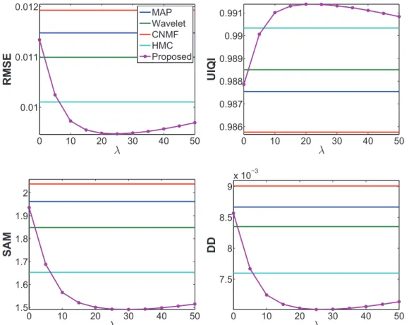
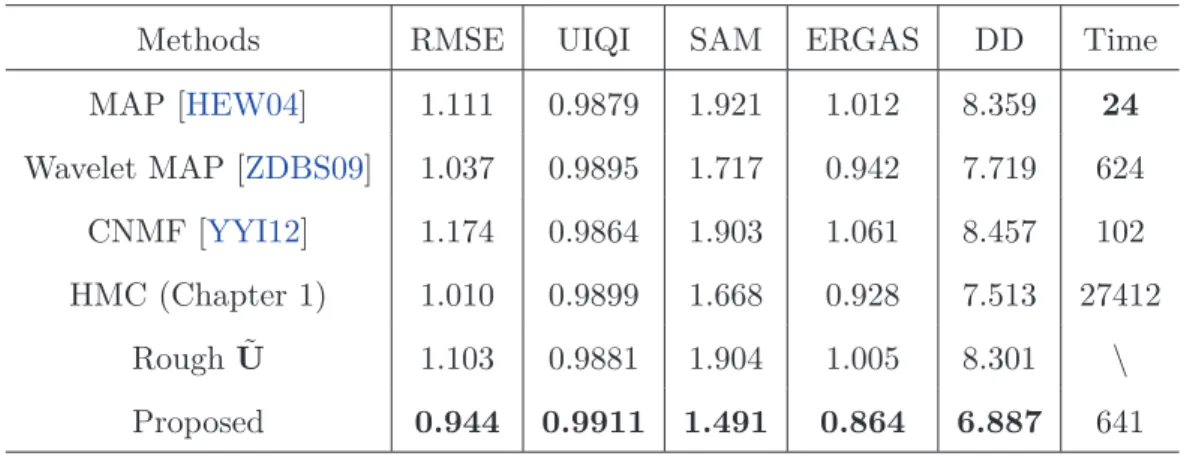
(Mid-dle 1) MAP [HEW04]. (Mid(Mid-dle 2) Wavelet MAP [ZDBS09]. (Mid(Mid-dle 3) CNMF fusion [YYI12]. (Middle 4) MCMC (Chapter 1). (Middle 5) Proposed method. (Bottom 1-5): The Corresponding RMSE maps. . . 66 2.7 Performance of the proposed fusion algorithm versus λ: (Top left) RMSE. (Top right)
UIQI. (Bottom left) SAM. (Bottom right) DD. . . 67 2.8 Whole Pavia dataset: (Top 1) Reference image. (Top 2) HS image. (Top 3) MS image.
(Middle 1) MAP [HEW04]. (Middle 2) Wavelet MAP [ZDBS09]. (Middle 3) CNMF
fusion [YYI12]. (Bottom 1) MCMC (Chapter 1). (Bottom 2) Rough estimation ˜U.
(Bottom 3) Proposed method. . . 68 2.9 LANDSAT-like spectral responses (4 bands in MS image). . . 70 2.10 Moffett dataset (HS+MS): (Top 1) Reference image. (Top 2) HS image. (Top 3) MS
image. (Middle 1) MAP [HEW04]. (Middle 2) Wavelet MAP [ZDBS09]. (Middle 3) CNMF fusion [YYI12]. (Bottom 1) MCMC (Chapter 1). (Bottom 2) Rough estimation
˜
U. (Bottom 3) Proposed method. . . 70 2.11 Moffett dataset (HS+PAN): (Top 1) Reference image. (Top 2) HS image. (Top 3) PAN
image. (Middle 1) MAP [HEW04]. (Middle 2) Wavelet MAP [ZDBS09]. (Middle 3) CNMF fusion [YYI12]. (Bottom 1) HMC (Chapter 1). (Bottom 2) Rough estimation
˜
U. (Bottom 3) Proposed method. . . 72 3.1 Pavia dataset: (Left) HS image. (Middle) MS image. (Right) reference image. . . 92
supervised naive Gaussian prior (1st column), unsupervised naive Gaussian prior (2nd column), sparse representation (3rd column) and TV (4th column). (Row 3 and 4) The corresponding RMSE maps. . . 96 3.3 Convergence speeds of the ADMM [SBDAC15] and the proposed FUSE-ADMM with
TV-regularization. . . 97 3.4 Observations and ground truth: (Left) scaled HS image. (Middle) PAN image. (Right)
Reference image. . . 98 3.5 Hyperspectral pansharpening results: (Row 1 and 2) The state-of-the-art-methods and
corresponding proposed fast fusion methods (FUSE), respectively, with various regu-larizations: supervised naive Gaussian prior (1st column), unsupervised naive Gaus-sian prior (2nd column), sparse representation (3rd column) and TV (4th column). (Row 3 and 4) The corresponding RMSE maps. . . 100 3.6 Madonna dataset: (Top left) HS image. (Top middle) PAN image. (Top right)
Refer-ence image. (Bottom left) Fusion with method in [HEW04]. (Bottom middle) Fusion
with ADMM in Chap. 1. (Bottom right) Fusion with proposed FUSE. . . 102
4.1 Hyperspectral pansharpening results (Moffet dataset): (Top 1) HS image. (Top 2) MS image. (Top 3) Reference image. (Middle 1) Berne’s method. (Middle 2) Yokoya’s method. (Middle 3) S-FUMI (Middle 4) UnS-FUMI. (Bottom 1-4) The corresponding RMSE maps. . . 127 4.2 Scattered Moffet data: The 1st and the 100th bands are selected as the coordinates. . 128 4.3 Unmixed endmembers for Madonna HS+PAN datasets: (Top and bottom left)
Esti-mated three endmembers and ground truth. (Bottom right) Sum of absolute value of all endmember errors as a function of wavelength. . . 129 4.4 Unmixed abundance maps for Madonna HS+PAN dataset: Estimated abundance
maps using (Row 1) Berne’s method, (Row 2) Yokoya’s method, and (Row 3) UnS-FUMI. (Row 4) Reference abundance maps. . . 131
image. (Top 3) Reference image. (Middle 1) Berne’s method. (Middle 2) Yokoya’s method. (Middle 3) S-FUMI method. (Middle 4) UnS-FUMI method. (Bottom 1-4) The corresponding RMSE maps. . . 132 4.6 Scattered Pavia data: The 30th and the 80th bands are selected as the coordinates. . 133 4.7 Unmixed endmembers for PAVIA HS+PAN dataset: (Top and bottom left) Estimated
three endmembers and ground truth. (Bottom right) Sum of absolute value of all endmember errors as a function of wavelength. . . 134 4.8 Unmixed abundance maps for PAVIA HS+PAN dataset: Estimated abundance maps
using (Row 1) Berne’s method, (Row 2) Yokoya’s method, and (Row 3) UnS-FUMI. (Row 4) Reference abundance maps. . . 135 B.1 Fusion results. (Top 1) Reference image. (Top 2) HS image. (Top 3) MS image.
(Middle 1) MAP [HEW04]. (Middle 2) Wavelet MAP [ZDBS09]. (Middle 3) MCMC with known R. (Middle 4) MCMC with unknown R. (Bottom 1-4) The corresponding RMSE maps. . . 164 B.2 True pseudo-spectral responseRå (top) and its estimation (bottom). . . 165
B.3 Noise variances and their MMSE estimates: (Top) HS Image. (Bottom) MS Image. . . 166
1 Some existing remote sensors characteristics . . . 4 2 Notations . . . 6 1.1 Performance of HS+MS fusion methods in terms of: RSNR (in dB), UIQI, SAM (deg),
ERGAS, DD(in 10−2) and time (in second) (AVIRIS dataset). . . 34
1.2 Performance of HS+PAN fusion methods in terms of: RSNR (in dB), UIQI, SAM (in degree), ERGAS, DD(in 10−2) and time (in second) (ROSIS dataset). . . 37
1.3 Performance of the compared fusion methods: RSNR (in dB), UIQI, SAM (in degree), ERGAS, DD (in 10−2) and time (in second) (AVIRIS dataset). . . 45
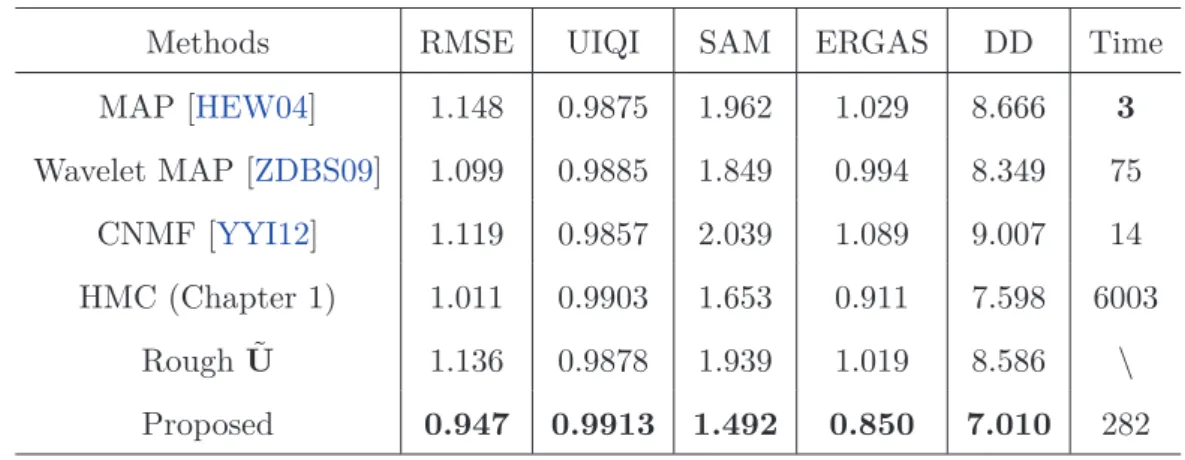
2.1 Performance of different MS + HS fusion methods (Pavia dataset): RMSE (in 10−2),
UIQI, SAM (in degree), ERGAS, DD (in 10−3) and Time (in second). . . 65
2.2 Performance of different MS + HS fusion methods (Whole Pavia dataset): RMSE (in 10−2), UIQI, SAM (in degree), ERGAS, DD (in 10−3) and Time (in second). . . 69
2.3 Performance of different MS + HS fusion methods (Moffett field): RMSE (in 10−2),
UIQI, SAM (in degree), ERGAS, DD (in 10−2) and Time (in second). . . 71
2.4 Performance of different Pansharpening (HS + PAN) methods (Moffett field): RMSE (in 10−2), UIQI, SAM (in degree), DD (in 10−2) and Time (in second). . . 71
3.1 Performance of HS+MS fusion methods: RSNR (in dB), UIQI, SAM (in degree), ERGAS, DD (in 10−3) and time (in second). . . 94
3.2 Performance of the Pansharpening methods: RSNR (in dB), UIQI, SAM (in degree), ERGAS, DD (in 10−2) and time (in second). . . 99
ERGAS, DD (in 10−3) and time (in second). . . 102
4.1 Fusion Performance for Synthetic HS+MS dataset: RSNR (in dB), UIQI, SAM (in degree), ERGAS, DD (in 10−3) and time (in second). . . 123
4.2 Unmixing Performance for Synthetic HS+MS dataset: SAMM (in degree), NMSEM
(in dB) and NMSEA (in dB). . . 123
4.3 Fusion Performance for Synthetic HS+PAN dataset: RSNR (in dB), UIQI, SAM (in degree), ERGAS, DD (in 10−3) and time (in second). . . 124
4.4 Unmixing Performance for Synthetic HS+PAN dataset: SAMM(in degree), NMSEM
(in dB) and NMSEA (in dB). . . 124
4.5 Fusion Performance for Moffet HS+PAN dataset: RSNR (in dB), UIQI, SAM (in degree), ERGAS, DD (in 10−2) and time (in second). . . 126
4.6 Unmixing Performance for Pavia HS+PAN dataset: SAMM (in degree), NMSEM (in
dB) and NMSEA (in dB). . . 126
4.7 Fusion Performance for Pavia HS+PAN dataset: RSNR (in dB), UIQI, SAM (in de-gree), ERGAS, DD (in 10−2) and time (in second). . . 130
4.8 Unmixing Performance for Pavia HS+PAN dataset: SAMM (in degree), NMSEM (in
dB) and NMSEA (in dB). . . 130
A.1 Notations Summary . . . 148 B.1 Performance of the compared fusion methods: RSNR (in db), UIQI, SAM (in degree),
ERGAS, DD (in 10−2) and Time (in second)(AVIRIS dataset). . . 166
1 Hybrid Gibbs sampler . . . 24 2 Hybrid Monte Carlo algorithm . . . 27 3 Adjusting stepsize . . . 32 4 Block Coordinated Descent algorithm . . . 39 5 SALSA step . . . 41 6 Fusion of HS and MS based on a sparse representation . . . 56 7 SALSA sub-iterations . . . 58
8 Fast fUsion of multi-band images based on solving a Sylvester Equation (FUSE) . . . 86
9 ADMM sub-iterations to estimate A . . . 114 10 Projecting (A − G)i onto the Simplex A . . . 116
11 ADMM steps to estimate M . . . 117 12 Joint Fusion and Unmixing for Multi-band Images(FUMI) . . . 119 13 Hybrid Gibbs sampler in vector form . . . 153 14 Hybrid Monte Carlo algorithm in vector form . . . 155 15 Hybrid Gibbs sampler with unknown R . . . 162
Context and objectives of the thesis
Background
In general, a multi-band image can be represented as a three-dimensional data cube indexed by three exploratory variables (x, y, λ), where x and y are the two spatial dimensions of the scene, and λ is the spectral dimension (covering a range of wavelengths), as is shown in Fig. 1. Typical examples of multi-band images include hyperspectral (HS) images [Lan02], multi-spectral (MS) images [Nav06], integral field spectrographs [BCM+01], magnetic resonance spectroscopy images etc. However,
multi-band imaging generally suffers from the limited spatial resolution of the data acquisition devices, mainly due to an unsurpassable tradeoff between spatial and spectral sensitivities [Cha07] as well as the atmospheric scattering, secondary illumination, changing viewing angles, sensor noise, etc.
As a consequence, the problem of fusing a high spatial and low spectral resolution image with an auxiliary image of higher spectral but lower spatial resolution, also known as multi-resolution image fusion, has been explored for many years and is still a challenging but very crucial and active research area in various scenarios [Wal99, DCLS07, ASN+08, AMV+11, Sta11a, GZM12, JD14, LAJ+]. A
live example is shown in Fig. 2.
When considering remotely sensed images, an archetypal fusion task is the pansharpening [THHC04,
GASCG04,ASN+08,JJ10,LY11], which generally consists of fusing a high spatial resolution
panchro-matic (PAN) image and low spatial resolution MS image. Pansharpening has been addressed in the
Figure 1: Hyperspectral data cube
literature for several decades and still remains an active topic [AMV+11,LB12,DJHP14]. More
re-cently, HS imaging, which consists of acquiring a same scene in several hundreds of contiguous spectral bands, has opened a new range of relevant applications, such as target detection [MS02], classification [C.-03], spectral unmixing [BDPD+12], and visualization [KC13]. However, while HS sensors provide
abundant spectral information, their spatial resolution is generally more limited [Cha07]. To take advantage of the newest benefits offered by HS images to obtain images with both good spectral and spatial resolutions, the remote sensing community has been devoting increasing research efforts to the problem of fusing HS with other highly-resolved MS or PAN images [CQAX12, HCBD+14].
In practice, the spectral bands of PAN images always cover the visible and infra-red spectra. How-ever, in several practical applications, the spectrum of MS data includes additional high-frequency spectral bands. For instance the MS data of WorldView-31 have spectral bands in the intervals
[400∼ 1750]nm and [2145 ∼ 2365]nm whereas the PAN data are in the range [450 ∼ 800]nm. More examples of HS and MS sensor resolutions are given in Table 1.
The problem of fusing HS and PAN images has been explored recently [CM09,LKC+12,LAJ+].
Capitalizing on decades of experience in MS pansharpening, most of the HS pansharpening ap-proaches merely adapt existing algorithms for PAN and MS fusion [MWB09, CPWJ14]. Other methods are specifically designed to the HS pansharpening problem (see, e.g., [WW02, CQAX12,
Figure 2: (Left) Hyperspectral image (size: 99 × 46 × 224, res.: 80m × 80m). (Middle) Panchromatic image (size: 396 × 184 res.: 20m × 20m). (Right) Target image (size: 396 × 184 × 224 res.: 20m × 20m).
LKC+12]). Conversely, the fusion of MS and HS images has been considered in fewer research works
and is still a challenging problem because of the high dimensionality of the data to be processed. In-deed, the fusion of HS and MS differs from traditional MS or HS pansharpening by the fact that more spatial and spectral information is contained in multi-band images. Therefore, a lot of pansharpening methods, such as component substitution [She92] and relative spectral contribution [ZCS98] are in-applicable or inefficient for the fusion of HS and MS images. Another motivation for this multi-band fusion problem is the HS+MS suite (called hyperspectral imager suite (HISUI)) that aims at fusing co-registered MS and HS images acquired over the same scene under the same conditions has been
Name AVIRIS (HS) SPOT-5 (MS) Pleiades (MS) WorldView-3 (MS)
Res. (m) 20 10 2 1.24
# bands 224 4 4 8
Table 1: Some existing remote sensors characteristics
developed by the Japanese ministry of economy, trade, and industry (METI) [OIKI10]. HISUI is the Japanese next-generation Earth-observing sensor composed of HS and MS imagers and will be launched by the H-IIA rocket in 2015 or later as one of mission instruments onboard JAXA’s ALOS-3 satellite. Some research activities have already been conducted for this practical multi-band fusion problem [YI13].
Note that in this thesis, the image fusion we are interesting in is the pixel-level fusion, in which the output is an image with increased information comparing with each input. However, there exist other aspects of image fusions, such as feature-level fusion, symbol-level fusion and decision-level fusion depending to the stage at which the fusion takes place [ZZVG06,Sta11b]. The choice of the appropriate level relies on the characteristics of sensory data, fusion application, and availability of tools [LK95]. Though these kinds of fusions are not considered in this thesis, they have recently attracted great interests in classification [FCB06], sub-pixel mapping [CKRS12], target detection [HFP+15], etc.
Problem formulation (matrix form)
To better distinguish spectral and spatial degradations, the pixels of the target multi-band image, which is of high-spatial and high-spectral resolution, can be rearranged to build an mλ× n matrix X, where mλ is the number of spectral bands and n = nr× nc is the number of pixels in each band (nr and nc represent the number of rows and columns respectively). In other words, each column of the matrix X consists of a mλ-valued pixel and each row gathers all the pixel values in a given spectral band. Note that in this thesis, the image X of interest is the hyperspectral image of reflectance data which takes values between 0 and 1.
Generally, the linear degradations of the observed images w.r.t. the target high-spatial and high-spectral image reduce to spatial and spectral transformations. Based on this pixel ordering, any linear operation applied to the left (resp. right) side of X describes a spectral (resp. spatial) degradation. Thus, the multi-band image fusion problem can be interpreted as restoring a three dimensional data-cube from two degraded data-cubes. A more precise description of the problem formulation is provided in what follows. Note that using matrix notations allows the fusion problem to be more easily formulated. The HS image, referred to as YH, is supposed to be a blurred,
down-sampled and noisy version of the target image X whereas the MS image, referred to as YM is a
spectrally degraded and noisy version of X. As a consequence, the observation models associated with the HS and MS images can be written as [MKM99,HEW04,MVMK08]
YH = XBS + NH
YM = RX + NM
(1)
where X = [x1,· · · , xn]∈ Rmλ×n is the unknown full resolution HS image composed of mλ bands and n pixels, YH∈ Rmλ×m is the HS image composed of mλ bands and m pixels and YM∈ Rnλ×n
is the MS image composed of nλ bands and n pixels. In (1), B ∈ Rn×n is a cyclic convolution operator acting on the bands that models the point spread function of the HS sensor and S ∈ Rn×m is a downsampling matrix (with downsampling factor denoted as d). Conversely, R ∈ Rnλ×mλ models the spectral response of the MS sensor, which is assumed to be unknown. The noise matrices NH ∈ Rmλ×m and NM ∈ Rnλ×n are assumed to be distributed according to the following matrix
Gaussian distributions [Daw81]
NH ∼ MNmλ,m(0mλ,m, ΛH, Im)
NM ∼ MNnλ,n(0nλ,n, ΛM, In)
(2)
where 0a,b is the a × b matrix of zeros, I·λ is the ·λ × ·λ identity matrix, ΛH = diag
! s2 H ", s2 H = è s2H,1, . . . , s2H,m λ éT , and ΛM= diag!s2M ", s2 M= è s2M,1, . . . , s2M,n λ éT
. In (2), MN represents the matrix normal distribution. The probability density function of a matrix normal distribution MN (M, Σr, Σc)
is defined by
p(X|M, Σr, Σc) =
exp1−12trèΣc−1(X− M)TΣ−1r (X− M)é2 (2π)np/2|Σ
c|n/2|Σr|p/2
where M denotes its mean and Σr and Σc are two matrices denoting row and column covariance ma-trices. To facilitate the reading, all matrix dimensions and their respective relations are summarized in Table2. Note that besides this popular matrix formulation, there exists a corresponding vectorized formulation, which vectorized all the multi-band image, such as in [WCJ+13,HCBD+14,WDT15a].
The equivalent formulation in vector form of the considered fusion problem is available in the Ap-pendix A.
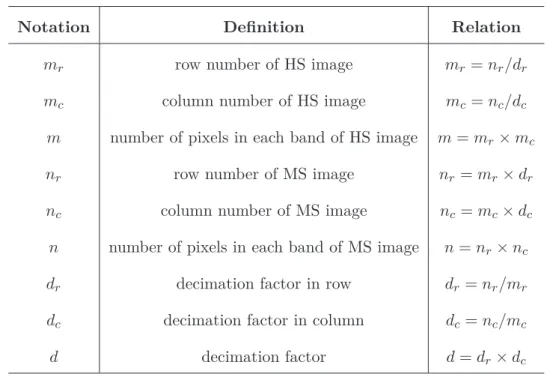
Table 2: Notations
Notation Definition Relation
mr row number of HS image mr= nr/dr
mc column number of HS image mc= nc/dc
m number of pixels in each band of HS image m = mr× mc
nr row number of MS image nr = mr× dr
nc column number of MS image nc = mc× dc
n number of pixels in each band of MS image n = nr× nc
dr decimation factor in row dr= nr/mr
dc decimation factor in column dc = nc/mc
d decimation factor d = dr× dc
Bayesian framework
Since the fusion problem is usually ill-posed, the Bayesian methodology offers a convenient way to regularize the problem by defining an appropriate prior distribution for the scene of interest. More
specifically, Bayesian fusion allows an intuitive interpretation of the fusion process via the posterior distribution. Following this strategy, Gaussian or ℓ2-norm priors have been considered to build
various estimators, in the image domain [HEW04,WDT15a,WDT14a] or in a transformed domain
[ZDBS09]. Recently, the fusion of HS and MS images based on spectral unmixing has also been
explored [YYI12,YCI12].
Furthermore, many strategies related to HS resolution enhancement have been proposed to define this prior distribution. For instance, in [JJ10], the highly resolved image to be estimated is a priori modeled by an in-homogeneous Gaussian Markov random field (IGMRF). The parameters of this IGMRF are empirically estimated from a panchromatic image in the first step of the analysis. In [HEW04] and related works [EH04,EH05], a multivariate Gaussian distribution is proposed as prior distribution for the unobserved scene. The resulting conditional mean and covariance matrix can then be inferred using a standard clustering technique [HEW04] or using a stochastic mixing model [EH04,
EH05], incorporating spectral mixing constraints to improve spectral accuracy in the estimated high resolution image.
Objective
To address the challenge raised by the high dimensionality, spatial degradation and spectral mixture of the data to be fused, innovative methods need to be developed, which is the main objective of this thesis.
In this thesis, we propose to explicitly exploit the acquisition process of the different images. More precisely, the sensor specifications (i.e., spectral or spatial responses) are exploited to properly design the spatial or spectral degradations suffered by the image to be recovered [OGAFN05]. Moreover, to define the prior distribution assigned to this image, we resort to geometrical considerations well admitted in the HS imaging literature devoted to the linear unmixing problem [DMC+09]. In
partic-ular, the high spatial resolution HS image to be estimated is assumed to live in a lower dimensional subspace, which is a suitable hypothesis when the observed scene is composed of a finite number of macroscopic materials.
the fusion problem are incorporated into the model via the prior distribution assigned to the scene to be estimated. Within a Bayesian estimation framework, two statistical estimators are generally considered. The minimum mean square error (MMSE) estimator is defined as the mean of the posterior distribution. Its computation generally requires intractable multidimensional integration. Conversely, the maximum a posteriori (MAP) estimator is defined as the mode of the posterior distribution and is usually associated with a penalized maximum likelihood approach. Mainly due to the complexity of the integration required by the computation of the MMSE estimator (especially in high-dimension data space), most Bayesian estimators proposed to solve the HS and MS fusion problem use a MAP formulation [HEW04, ZDBS09, JBC06]. In general, optimization algorithms designed to maximize the posterior distribution are computationally efficient but they may suffer from the presence of local extrema, that prevents any guarantee to converge towards the actual maximum of the posterior. The MMSE estimator can overcome the local extrema problem but demands much more expensive computational burden. In this thesis, both estimators are explored to solve the Bayesian fusion problem.
Organization of the manuscript
• Chapter 1: This chapter is interested in a Bayesian fusion technique for remotely sensed multi-band images, including the HS, MS and PAN images [WDT15a,WDT14a,WDT15c,WDT14b]. First, the fusion problem is formulated within a hierarchical Bayesian estimation framework, by introducing the general forward model and statistical assumptions for the observed multi-band images. An appropriate Gaussian prior distribution exploiting geometrical consideration is introduced. To approximate the Bayesian estimator of the scene of interest from its posterior distribution, a Markov chain Monte Carlo (MCMC) algorithm (more precisely a hybrid Gibbs sampler) is proposed to generate samples asymptotically distributed according to the target distribution. To efficiently sample from this high-dimension distribution, a Hamiltonian Monte Carlo step is introduced within a Gibbs sampling strategy. The efficiency of the proposed fusion method is evaluated with respect to (w.r.t.) several state-of-the-art fusion techniques. Secondly,
an optimization based counterpart of the proposed Bayesian statistical method, consisting of an alternating direction method of multipliers (ADMM) within block coordinate descent (BCD) algorithm is developed to decrease the computational complexity. Besides, an extension of this work to the case where the sensor spectral response is unknown is available in Appendix B.
• Chapter 2: In this chapter, we develop a variational-based approach for fusing HS and MS images [WBDDT15,WDT14c]. The fusion problem is formulated as an inverse problem whose solution is the target image that is assumed to live in a lower dimensional subspace. A sparse regularization term is carefully designed, ensuring that the target image is well represented by a linear combination of atoms belonging to an appropriate dictionary. The dictionary atoms and the supports of the corresponding active coding coefficients are a priori learned from the observed images. Then, conditionally on these dictionaries and supports, the fusion problem is solved via alternating optimization with respect to the target image (using the ADMM) and the coding coefficients. Compared with other state-of-the-art fusion methods, the proposed fusion method shows smaller spatial error and smaller spectral distortion with a reasonable computation complexity [LAJ+]. This improvement is attributed to the specific sparse prior
designed to regularize the resulting inverse problem.
• Chapter 3: This chapter studies a fast multi-band image fusion algorithm [WDT15d,WDT15e]. Following the well admitted forward model and the corresponding likelihoods of the observa-tions introduced in Chapter 1, maximizing the target distribution is equivalent to solving a Sylvester matrix equation. By exploiting the properties of the circulant and downsampling matrices associated with the fusion problem, a closed-form solution of this Sylvester equation is obtained, getting rid of any iterative update step. Coupled with the ADMM and the BCD method, the proposed algorithm can be easily generalized to incorporate some prior information for the fusion problem, such as the ones derived in Chapters 2 and 3 and [SBDAC15]. Sim-ulation results show that the proposed algorithm achieves the same performance as previous algorithms as well as the one in [SBDAC15], with the advantage of significantly decreasing the computational complexity of these algorithms.
• Chapter 4:
In this chapter, we propose a multi-band image fusion algorithm based on unsupervised spec-tral unmixing [WBDDTb]. We decompose any image pixel as a linear mixture of endmembers weighted by their abundances. The non-negativity and sum-to-one constraints are introduced for the abundances whereas the non-negativity is imposed to the endmembers. A joint fu-sion and unmixing strategy is introduced, leading to a maximization of the joint posterior distribution w.r.t. the abundances and endmember signatures, which can be solved using an alternating optimization algorithm. Thanks to the fast fusion algorithm based on solving the associated Sylvester equation presented in Chapter 3, the optimization w.r.t. the abundances can be solved efficiently. Simulation results show that the proposed joint fusion and unmixing strategy improves both the unmixing performance as well as the fusion performance compared with the results obtained with some state-of-the-art joint fusion and unmixing algorithms.
• Appendix D:
This appendix presents a fast spectral unmixing algorithm based on Dykstra’s alternating pro-jection. The proposed algorithm formulates the fully constrained least squares optimization problem associated with the spectral unmixing task as an unconstrained regression problem followed by a projection onto the intersection of several closed convex sets. This projection is achieved by iteratively projecting onto each of the convex sets individually, following Dyk-tra’s scheme. The sequence thus obtained is guaranteed to converge to the sought projection. Thanks to the preliminary matrix decomposition and variable substitution, the projection is implemented intrinsically in a subspace, whose dimension is very often much lower than the number of bands. A benefit of this strategy is that the order of the computational complex-ity for each projection is decreased from quadratic to linear time. Numerical experiments considering diverse spectral unmixing scenarios provide evidence that the proposed algorithm competes with the state-of-the-art, namely when the number of endmembers is relatively small, a circumstance often observed in real hyperspectral applications.
Main Contributions
The main contributions of this thesis are
• Chapter 1. A hierarchical Bayesian framework is proposed for multi-band image fusion
[WDT15a, WDT14b, WDT15c]. Two solutions are developed to evaluate the resulting
pos-terior distribution of interest. From the simulation-based perspective, a Hamiltonian Monte Carlo within Gibbs sampler is designed to generate samples asymptotically distributed accord-ing to the target distribution. From the optimization perspective, an ADMM within BCD algorithm is developed to maximize the posterior.
• Chapter 2. A sparse regularization using dictionaries learned from the observed images is in-corporated to regularize the ill-posed problem [WBDDT15,WDT14c]. Identifying the supports jointly with the dictionaries circumvented the difficulty inherent to sparse coding. An alternate optimization algorithm, consisting of an ADMM and a least square regression, is designed to minimize the target function.
• Chapter 3. A closed-form solution for the Sylvester matrix equation associated with maxi-mizing the likelihood of the target image is obtained by exploiting the properties of the blur-ring and downsampling matrices in the fusion problem, getting rid of any iterative update step [WDT15d, WDT15e]. The proposed solution can be embedded in an ADMM or a BCD method to incorporate different priors or hyper-priors for the fusion problem, allowing alternate Bayesian estimators to be considered.
• Chapter 4. A joint multi-band image fusion and unmixing scheme is proposed by combining the well admitted linear spectral mixture model and the forward model used in the first three chapters [WBDDTb]. The non-negativity and sum-to-one constraints resulted from the intrinsic physical properties of the abundances are introduced as prior information to regularize this ill-posed problem. The joint fusion and unmixing problem is solved in an alternating optimization framework, mainly consisting of solving a Sylvester equation and projecting onto a simplex.
Papers in preparation
1. Q. Wei, J. M. Bioucas-Dias, N. Dobigeon and J-Y. Tourneret, Multi-band image fusion based on spectral unmixing, in preparation.
Submitted papers
1. Q. Wei, J. M. Bioucas-Dias, N. Dobigeon and J-Y. Tourneret, Fast spectral unmixing based on Dykstra’s alternating projection, IEEE Trans. Signal Process., under review.
International Journal papers
1. Q. Wei, N. Dobigeon and J-Y. Tourneret, Fast fusion of multi-band images based on solving a Sylvester equation, IEEE Trans. Image Process., vol. 24, no. 11, pp. 4109-4121, Nov. 2015.
2. L. Loncan, L. B. Almeida, J. M. Bioucas-Dias, X. Briottet, J. Chanussot, N. Dobigeon, S. Fabre, W. Liao, G. Licciardi, M. Simoes, J-Y. Tourneret, M. Veganzones, G. Vivone, Q. Wei and N. Yokoya, Hyperspectral pansharpening: a review, IEEE Geosci. and Remote Sens.
Mag., to appear.
3. Q. Wei, N. Dobigeon and J-Y. Tourneret, Bayesian fusion of multi-band images, IEEE J.
Sel. Topics Signal Process., vol. 9, no. 6, pp. 1117-1127, Sept. 2015.
4. Q. Wei, J. M. Bioucas-Dias, N. Dobigeon and J-Y. Tourneret, Hyperspectral and multi-spectral image fusion based on a sparse representation, IEEE Trans. Geosci. and
Remote Sens., vol. 53, no. 7, pp. 3658-3668, Jul. 2015.
Conference papers
1. Qi Wei, Nicolas Dobigeon and Jean-Yves Tourneret, FUSE: A Fast Multi-Band Image Fusion Algorithm, in Proc. IEEE Int. Workshop Comput. Adv. Multi-Sensor Adaptive
Process. (CAMSAP), Cancun, Mexico, Dec. 2015, to appear.
2. L. Loncan, L. B. Almeida, J. M. Bioucas-Dias, X. Briottet, J. Chanussot, N. Dobigeon, S. Fabre, W. Liao, G. Licciardi, M. Simoes, J-Y. Tourneret, M. Veganzones, G. Vivone, Q. Wei and N. Yokoya, Comparison of Nine Hyperspectral Pansharpening Methods, in Proc.
IEEE Int. Geosci. Remote Sens. Symp. (IGARSS), Milan, Italy, Jul. 2015, to appear.
3. Q. Wei, N. Dobigeon and J-Y. Tourneret, Bayesian fusion of multispectral and hyper-spectral images using a block coordinate descent Method, in Proc. IEEE GRSS
Work-shop Hyperspectral Image SIgnal Process.: Evolution in Remote Sens.(WHISPERS), Tokyo,
Japan, Jun. 2015, to appear. Note: Invited paper.
4. Q. Wei, N. Dobigeon and J-Y. Tourneret, Bayesian fusion of multispectral and hyper-spectral images with unknown sensor hyper-spectral response, in Proc. IEEE Int. Conf.
Image Processing (ICIP), Paris, France, Oct. 2014, pp. 698-702. Note: Invited paper.
5. Q. Wei, J. M. Bioucas-Dias, N. Dobigeon and J-Y. Tourneret, Fusion of multispectral and hyperspectral images based on sparse representation, in Proc. European Signal
Pro-cessing Conf. (EUSIPCO), Lisbon, Portugal, Sept. 2014, pp. 1577-1581. Note: Invited paper.
6. Q. Wei, N. Dobigeon and J-Y. Tourneret, Bayesian fusion of hyperspectral and multi-spectral images, in Proc. IEEE Int. Conf. Acoust., Speech, and Signal Processing (ICASSP),
Florence, Italy, May 2014, pp. 3200-3204. Note: Awarded IEEE SPS Travel Grant.
Other publications related to previous works
1. J. Vilà-Valls, Q. Wei, P. Closas and C. Fernandez-Prades, Robust Gaussian Sum Filtering with Unknown Noise Statistics: application to target tracking, in IEEE Statistical
Signal Processing Workshop (SSP’14), Gold Coast, Australia, June 2014, pp. 416-419. Note:
Invited paper.
2. Q. Wei, T. Jin and F. Yu, Effective frequency selection algorithm for bandpass sam-pling of multiband RF signals based on relative frequency interval, in International
Conference on Computer Application and System Modeling (ICCASM), Taiyuan, China, Oct.
Bayesian fusion of multi-band images
using a Gaussian prior
Part of this chapter has been adapted from the journal paper [WDT15a] (published) and the conference papers [WDT14a] (published), [WDT14b] (published) and [WDT15c] (published).
Contents
1.1 Introduction . . . . 18 1.1.1 Bayesian estimation of X . . . 19 1.1.2 Lower-dimensional subspace . . . 20 1.1.3 Likelihood and prior distributions . . . 21 1.1.4 Hyperparameter prior . . . 22 1.1.5 Posterior distribution . . . 22 1.1.6 Inferring the highly-resolved HS image from the posterior of U . . . 23 1.1.7 Hybrid Gibbs sampler . . . 24 1.1.8 Complexity analysis . . . 28 1.2 Simulation results (MCMC algorithm) . . . . 28 1.2.1 Fusion of HS and MS images . . . 28 1.2.2 Stepsize and leapfrog steps . . . 31 1.2.3 Evaluation of the fusion quality . . . 32 1.2.4 Comparison with other Bayesian models . . . 34 1.2.5 Estimation of the noise variances . . . 35 1.2.6 Robustness with respect to the knowledge of R . . . 35 1.2.7 Application to Pansharpening . . . 36 1.3 Block Coordinate Descent method . . . . 38 1.3.1 Optimization with respect to U . . . 39 1.3.2 Optimization with respect to s2 . . . 40 1.3.3 Optimization with respect to Σ . . . 41 1.3.4 Relationship with the MCMC method . . . 42 1.4 Simulation results (BCD algorithm) . . . . 42 1.4.1 Simulation scenario . . . 42
1.4.2 Hyperparameter selection . . . 44 1.4.3 Fusion performance . . . 44 1.5 Conclusion . . . . 46
1.1
Introduction
In this chapter, a prior knowledge accounting for artificial constraints related to the fusion problem is incorporated within the model via the prior distribution assigned to the scene to be estimated. Many strategies related to HS resolution enhancement have been proposed to define this prior dis-tribution. For instance, in [JJ10], the highly resolved image to be estimated is a priori modeled by an in-homogeneous Gaussian Markov random field (IGMRF). The parameters of this IGMRF are empirically estimated from a panchromatic image in the first step of the analysis. In [HEW04] and related works [EH04, EH05], a multivariate Gaussian distribution is proposed as prior distribution for the unobserved scene. The resulting conditional mean and covariance matrix can then be inferred using a standard clustering technique [HEW04] or using a stochastic mixing model [EH04,EH05], in-corporating spectral mixing constraints to improve spectral accuracy in the estimated high resolution image.
In this chapter, we propose to explicitly exploit the acquisition process of the different images. More precisely, the sensor specifications (i.e., spectral or spatial responses) are exploited to properly design the spatial or spectral degradations suffered by the image to be recovered [OGAFN05]. More-over, to define the prior distribution assigned to this image, we resort to geometrical considerations well admitted in the HS imaging literature devoted to the linear unmixing problem [DMC+09]. In
particular, the high spatial resolution HS image to be estimated is assumed to live in a lower dimen-sional subspace, which is an admissible hypothesis when the observed scene is composed of a finite number of macroscopic materials.
Within a Bayesian estimation framework, two statistical estimators are generally considered. The MMSE estimator is defined as the mean of the posterior distribution. Its computation generally requires an intractable multidimensional integration. Conversely, the MAP estimator is defined as the
mode of the posterior distribution and is usually associated with a penalized maximum likelihood approach. Mainly due to the complexity of the integration required by the computation of the MMSE estimator (especially in high-dimension data space), most of the Bayesian estimators have proposed to solve the HS and MS fusion problem using a MAP formulation [HEW04, ZDBS09,
JBC06]. However, optimization algorithms designed to maximize the posterior distribution may
suffer from the presence of local extrema, that prevents any guarantee to converge towards the actual maximum of the posterior. In this work, we propose to approximate the Bayesian estimators of the unknown scene by using samples generated by an MCMC algorithm. The posterior distribution resulting from the proposed forward model and the a priori modeling is defined in a high dimensional space, which makes difficult the use of any conventional MCMC algorithm, e.g., the Gibbs sampler or the Metropolis-Hastings sampler [RC04]. To overcome this difficulty, a particular MCMC scheme, called Hamiltonian Monte Carlo (HMC) algorithm, is derived [DKPR87,Nea10]. It differs from the standard Metropolis-Hastings algorithm by exploiting Hamiltonian evolution dynamics to propose states with higher acceptance ratio, reducing the correlation between successive samples. Finally, the MMSE estimation for unknown parameters can be both computed from generated samples.
Thus, the main contributions of this chapter are two-fold. First, this chapter introduces a new hierarchical Bayesian fusion model whose parameters and hyperparameters have to be estimated from the observed images. This model is defined by the likelihood, the priors and the hyper-priors detailed in the following sections. Second, a hybrid Gibbs sampler based on a Hamiltonian MCMC method is introduced to sample the desired posterior distribution. These samples are subsequently used to approximate the MMSE estimator of the fused image.
1.1.1 Bayesian estimation of X
In this work, we propose to estimate the unknown scene X within a Bayesian estimation framework following the model (1). In this statistical estimation scheme, the fused highly-resolved image X is inferred through its posterior distribution f (X|Y), where Y = {YH, YM} contains the two observed
images. Given the observed data, this target distribution can be derived from the likelihood function
∝ means “proportional to”. Based on the posterior distribution, several estimators of the scene X can be investigated. For instance, maximizing f (X|Y) leads to the MAP estimator
ˆ
XMAP= arg max
X f (X|Y) . (1.1)
This estimator has been widely exploited for HS image enhancement (see for instance [HEW04,
EH04, EH05] or more recently [JJ10, ZDBS09]). This work proposes to focus on the first moment of the posterior distribution f (X|Y), which is known as the posterior mean estimator or the MMSE estimator ˆXMMSE. This estimator is defined as
ˆ XMMSE= Ú Xf (X|Y) dX = s Xf (Y|X) f (X) dX s f (Y|X) f (X) dX . (1.2) In order to compute (1.2), we propose a flexible and relevant statistical model to solve the fusion problem. Deriving the corresponding Bayesian estimators ˆXMMSE defined in (1.2), requires the
definition of the likelihood function f (Y|X) and the prior distribution f (X). These quantities are detailed in the next section.
1.1.2 Lower-dimensional subspace
The unknown image is X = [x1, . . . , xn] where xi = [xi,1, xi,2, . . . , xi,mλ]
T is the m
λ × 1 vector corresponding to the ith spatial location (with i = 1, . . . , n). Because the HS bands are spectrally correlated, the HS vector xi usually lives in a space whose dimension is much smaller than mλ [BDN08]. This property has been extensively exploited when analyzing HS data, in particular to perform spectral unmixing [BDPD+12]. More precisely, the HS image can be rewritten as X =
HU where H ∈ Rmλ×måλ has full column rank and U ∈ Rmåλ×n is the projection of X onto the subspace spanned by the columns of H. Incorporating this decomposition of the HS image X into the observation model (1) leads to
YH= HUBS + NH
YM= RHU + NM.
1.1.3 Likelihood and prior distributions
Likelihoods: Using the statistical properties of the matrices NH and NM, the distributions of YH
and YM are matrix Gaussian distributions, i.e.,
YH∼ MNmλ,m(HUBS, ΛH, Im)
YM∼ MNnλ,n(RHU, ΛM, In).
(1.4)
As the observed HS and MS images are acquired by different heterogeneous sensors, YHand YM
are assumed to be independent, conditionally upon the unobserved scene U and the noise covariances
s2=)s2 H, s2M
*. As a consequence, the joint likelihood function of the observed data is
f1Y|U, s22= f1YH|U, s2H
2
f1YM|U, s2M
2
(1.5)
Using the change of variables X = HU, the unknown parameters to be estimated to solve the fusion problem are the projected scene U and the vector of noise variances s2 = {s2
H, s2M}. The
appropriate prior distributions assigned to these parameters are presented below.
Scene prior: A Gaussian prior distribution is assigned to the projected image U, assuming that its column vectors ui for i = 1, · · · , n are spatially a priori independent, i.e.,
p(U) =MNmåλ,n(µ, Σ, In) (1.6)
where µ and Σ are the mean and covariance matrix of the matrix normal distribution. The Gaussian prior assigned to U implies that the target image U is a priori not too far from the mean vector
µ, whereas the covariance matrix Σ tells us how much confidence we have for the prior. In this
work, µ is fixed using the interpolated HS image in the subspace of interest following the strategy investigated in [HEW04] and Σ is an unknown hyperparameter to be estimated jointly with U.
Choosing a Gaussian prior for the matrix U is also motivated by the fact that this kind of prior has been used successfully in several works related to the fusion of multiple degraded images, including [HBA97,EH04,WGK06]. Note finally that the Gaussian prior has the interest of being a conjugate distribution relative to the statistical model (1.5). As it will be shown in Section 1.1.7, coupling
this Gaussian prior distribution with the Gaussian likelihood function leads to simpler estimators constructed from the posterior distribution f (U|Y).
Noise variance priors:
Conjugate inverse-gamma distributions are chosen as prior distributions for the noise variances
s2 H,i and s2M,j s2 H,i|νH, γH∼ IG!ν2H,γ2H", i = 1,· · · , mλ sM,i2 |νM, γM∼ IG!ν2M,γ2M", i = 1,· · · , nλ. (1.7)
The hyperparameters νH, γH, νMand γMcan be fixed to generate an informative or non-informative
prior, depending on the applications. In this work, they are fixed in order to obtain a non-informative prior.
1.1.4 Hyperparameter prior
The hyperparameter vector associated with the parameter priors defined above is Φ = {Σ}. Hyperparameter Σ:
Assigning a conjugate a priori inverse-Wishart distribution to the covariance matrix of a Gaussian vector has provided interesting results in the signal and image processing literature [DTI08, BF13]. Following these works, we have chosen the following prior for Σ
Σ∼ IW(Ψ, η) (1.8) whose density is f (Σ|Ψ, η) = |Ψ| η 2 2ηmλå2 Γ å mλ( η 2) |Σ|−η+mλ+1å2 e−12tr(ΨΣ −1) .
The parameters (Ψ, η)T are fixed to provide a non-informative prior for Σ.
1.1.5 Posterior distribution
The unknown parameter vector θ associated with the proposed hierarchical Bayesian fusion model is composed of the projected scene U and the noise variances s2, i.e., θ =)U, s2*. The joint posterior
distribution of the unknown parameters and hyperparameters can be computed using the following hierarchical structure
f (θ, Φ|Y) ∝ f (Y|θ) f (θ|Φ) f (Φ) (1.9) where the parameter and hyperparameter priors are given by
f (θ|Φ) = f (U|Σ) f!s2H"f!s2M" f (Φ) = f (Σ) .
(1.10)
1.1.6 Inferring the highly-resolved HS image from the posterior of U
The posterior distribution of the projected target image U, required to compute the Bayesian esti-mators (1.2), is obtained by marginalizing out the hyperparameter vector Φ and the noise variances
s2 from the joint posterior distribution f (θ, Φ|Y)
f (U|Y) ∝
Ú
f (θ, Φ|Y) dΦds2. (1.11)
The posterior distribution (1.11) is too complex to obtain closed-form expressions of the MMSE and MAP estimators ˆUMMSE and ˆUMAP. As an alternative, we propose to use an MCMC algorithm
to generate a collection of NMC samples U =
î
˜
U1, . . . , ˜UNMC ï
that are asymptotically distributed according to the posterior of interest f (U|Y). These samples will be used to compute the Bayesian estimators of U. More precisely, the MMSE estimator of U will be approximated by an empirical average of the generated samples ˜Ut
ˆ UMMSE ≈ 1 NMC− Nbi NØMC t=Nbi+1 ˜ Ut (1.12)
where Nbiis the number of burn-in iterations. Once the MMSE estimate ˆUMMSEhas been computed,
the highly-resolved HS image can be computed as ˆXMMSE = H ˆUMMSE. Sampling directly according
to the marginal posterior distribution f (U|Y) is not straightforward. Instead, we propose to sample according to the joint posterior f!U, s2, Σ|Y" by using a Metropolis-within-Gibbs sampler, which
can be easily implemented since all the conditional distributions associated with f!U, s2, Σ|Y"are relatively simple. The resulting hybrid Gibbs sampler is detailed in the following section.

![Figure 1.7: ROSIS dataset: (Top left) Reference image. (Top right) PAN image. (Middle left) Adaptive IHS [RSM + 10]](https://thumb-eu.123doks.com/thumbv2/123doknet/3187567.91036/67.892.177.742.211.667/figure-rosis-dataset-reference-image-right-middle-adaptive.webp)