HAL Id: insu-01769448
https://hal-insu.archives-ouvertes.fr/insu-01769448
Submitted on 18 Apr 2018
HAL is a multi-disciplinary open access
archive for the deposit and dissemination of
sci-entific research documents, whether they are
pub-lished or not. The documents may come from
teaching and research institutions in France or
abroad, or from public or private research centers.
L’archive ouverte pluridisciplinaire HAL, est
destinée au dépôt et à la diffusion de documents
scientifiques de niveau recherche, publiés ou non,
émanant des établissements d’enseignement et de
recherche français ou étrangers, des laboratoires
publics ou privés.
building
Philippe Lanos, Anne Philippe
To cite this version:
Philippe Lanos, Anne Philippe. Event date model: a robust Bayesian tool for chronology building.
Communications for Statistical Applications and Methods, Korean Statistical Society (KSS) /Korean
International Statistical Society (KISS), 2018, 25 (2), pp.131-157. �10.29220/CSAM.2018.25.2.131�.
�insu-01769448�
Event date model: a robust Bayesian tool for
chronology building
Lanos Philippea, Philippe Anne1,b
aIRAMAT-CRPAA, Universit ´e Bordeaux-Montaigne and G ´eosciences-Rennes, France; bLaboratoire de math ´ematiques Jean Leray, Universit ´e Nantes, France
Abstract
We propose a robust event date model to estimate the date of a target event by a combination of individual dates obtained from archaeological artifacts assumed to be contemporaneous. These dates are affected by errors of different types: laboratory and calibration curve errors, irreducible errors related to contaminations, and tapho-nomic disturbances, hence the possible presence of outliers. Modeling based on a hierarchical Bayesian statistical approach provides a simple way to automatically penalize outlying data without having to remove them from the dataset. Prior information on individual irreducible errors is introduced using a uniform shrinkage density with minimal assumptions about Bayesian parameters. We show that the event date model is more robust than models implemented in BCal or OxCal, although it generally yields less precise credibility intervals. The model is ex-tended in the case of stratigraphic sequences that involve several events with temporal order constraints (relative dating), or with duration, hiatus constraints. Calculations are based on Markov chain Monte Carlo (MCMC) numerical techniques and can be performed using ChronoModel software which is freeware, open source and cross-platform. Features of the software are presented in Vibet et al. (ChronoModel v1.5 user’s manual, 2016). We finally compare our prior on event dates implemented in the ChronoModel with the prior in BCal and OxCal which involves supplementary parameters defined as boundaries to phases or sequences.
Keywords: target event date model, robust combination of dates, hierarchical Bayesian statistics, MCMC computation, Chrono Model software
1. Introduction
Bayesian chronological modeling appears as an important issue in archeology and palaeo-environ mental science. This methodology has been developed since the 1990s (Bayliss, 2009, 2015) and is now the method of choice for the interpretation of radiocarbon dates. Most applications are undertaken using the flexible software packages, BCal (Buck et al., 1999), DateLab (Nicholls and Jones, 2002) and OxCal (Bronk Ramsey, 1995, 1998, 2001, 2008, 2009a,b; Bronk Ramsey et al., 2001, 2010; Bronk Ramsey and Lee, 2013).
All of these models provide an estimation of a chronology of dated events (DE), the estimated dates correspond to the dates of events that are actually dated by any chronometric technique. How-ever calibrated radiocarbon dates and date estimates from other chronometric dating methods such as thermoluminescence, archaeomagnetism, and dendrochronology. can be combined with various prior archeological information to produce a combined chronology that should be more reliable than its individual components.
1Corresponding author: Laboratoire de math´ematiques Jean Leray, Universit´e Nantes, UFR Sciences et techniques 2 rue
de la Houssiniere 44322 Nantes, France. E-mail: [email protected]
Published 31 March 2018/ journal homepage: http://csam.or.kr c
We propose a new chronological Bayesian model based on the concept of a target event. This is related to the concepts of the dated event and the target event proposed by Dean (1978). The target event (TE) is the event to which the date is to be applied by the chronometrician. Usually, the target events are not directly related to the dated events. According to Dean (1978), the dated event is contemporaneous with the target event when there is convergence (the two dates are coeval: DE = TE) and when the date is relevant to the target event. Relevance refers to the degree to which the date is applicable to the TE : it must be demonstrated or argued based on archaeological or other evidence. It is generally not easy or possible to assure the relevance of the dated event to the target event date of interest; therefore, it is recommended to get many dates of the dated event, and if possible from different dating techniques.
These dates can be outliers without having a means to determine if they are dating anomalies. In other words, we do not have any convincing archaeological arguments for rejecting them before modeling. This motivates the development of a robust statistical model for combining theses dates in such a way that it is very little sensitive to outliers (Lanos and Philippe, 2017).
The target event model is a statistical model introduced in (Lanos and Philippe, 2017) for estimat-ing the date of an event called a target event. This model allows to combine in a robust way the dates of artifacts, which are assumed to be contemporary to this target event. To validate the robustness of this model to outliers, we provide a comparison of our model with the t-type outlier model implemented in an Oxcal application. Numerical experiments also illustrate the sensibility to the outliers.
The target event model is then integrated to a global model for constructing chronologies of target events. Prior information is brought upon the dates of the target events. We show how the prior arche-ological information based on relative dating between the target events (in a stratigraphic sequence for instance) or based on duration, hiatus or terminus post quem (TPQ) or terminus ante quem (TAQ), assessment can be included in the model. The simulations and applications illustrates the improve-ment brought in term of robustness. The proposed model is impleimprove-mented in ChronoModel software, whose features are described in Vibet et al. (2016). This model can be compared with the standard chronological models when the target event is associated to only one dated event. However the inter-est of our approach is to get a robust inter-estimation of the date of target event even if the dated events embedded dated events are outliers. We compare in the simulation part this approach with an outlier model based using discrete mixture distributions.
Many issues in archaeology raise the problem of phasing or how to characterize the beginning, the end and the duration of a given period. This question can be viewed as a post processing of the chronological model as in Philippe and Vibet (2017a), Gu´erin et al. (2017). It is also possible to include additional parameters to characterize the phases. This requires the construction of a prior distribution on the dates of dated events that belong to the phase. This point is discussed in this paper, we analyze the choice of model implemented in an Oxcal application. We get an explicit form for the prior distribution of the dates, and we show that this probability distribution behaves in the same way as the dates included in a target event in the sense that we observe a concentration of dates belonging to the phase. Our result also shows the difficulty to construct appropriate prior on a sequence of dates.
The paper is organized as: In Section 2 we recall the construction of the target event model and we provide a theoretical comparison with the t-outlier model. In Section 3 we propose a new Bayesian model to estimate dates of target event. In Section 4, we analyze the Bayesian modelling of phases implemented in Oxcal application, and we compare this model with the target event model. In Sections 5 and 6 we apply our models to simulated and real datasets.
2. A robust combination of dates: the target event date model
We propose a statistical Bayesian approach for combining dates, which is based on a robust statistical model. This combination of dates is aiming to date a target event defined on the basis of archaeo-logical/historical arguments.
2.1. Description of the Bayesian model
We propose to use a hierarchical Bayesian model to estimate the date θ of a target event (Et). It combines dates ti (i= 1, . . . , n) of dated events (Ed) in such a way that it is robust to outliers. This
model is based on very few assumptions and does not need to tune hyper-parameters. It is described as follows.
The event dates tiare estimated from n independent measurements (observations, also called
de-terminations in Buck’s terminology) Miyielded by the different chronometric techniques. Each
mea-surement Mi, obtained from a specific dating technique, can be related to an individual date tithrough
a calibration curve gi and its error σgi (Lanos and Philippe, 2017, Section 2). Here this curve is
supposedly known with some known uncertainty.
At this step, the random effect model can be written as:
Mi= µi+ siϵi, ∀ i = 1, . . . , n,
µi= gi(ti)+ σgi(ti)ρi, (2.1)
where (ϵ1, . . . , ϵn, ρ1, . . . , ρn) are independent and identically Gaussian distributed random variables
with zero mean and variance 1, and where :
• siϵirepresents the experimental error provided by the laboratory.
• σgi(ti)ρirepresents the error provided by the calibration curve.
We assume that the experimental error provided by the laboratory are independent. Dependence structure could be added between the (siϵi)i=1,...,n in order to take into account the systematic error
associated to the dating techniques of each laboratory (Comb`es and Philippe (2017) in the particular case of the optically stimulated luminescence dating). However the construction of such a model requires additional information depending on each dating method and each laboratory, which is not available in most of the applications for chronological models.
Remark 1. If we assume that all the measurements can be calibrated with a common calibration
curve (i.e., gi = g for all i = 1, . . . , n), for example when the same object is analyzed by different
laboratories, the measurements can be combined according to the R-combine model (Bronk Ramsey, 2009b) before being incorporated in the event date model. This model can be viewed as a degenerated version of the target event model by takingσi = 0 for all i. On the contrary, if several calibration
curves are involved, the R-combine model is no longer valid and chronometric dates are directly incorporated in the event date model.
The target event dateθ is estimated from the dated events ti. The main assumption we make is
the contemporaneity (relevance and convergence, following Dean (1978)), of the dates ti with the
event date θ. However, because of error sources of unknown origin, it can exist an over-dispersion or dating anomalies of the dates with respect toθ. These errors can come from a method to ensure that the samples studied can provide realistic results for the events that we wish to characterize, the
care in sampling in the field, the care in sample handling, preparation and measure in the laboratory, or other non-controllable random factors that can appear during the process (Christen, 1994). This over-dispersion is also similar to the irreducible error described in (Niu et al., 2013) in the framework of radiocarbon calibration curve building.
Consequently, we model the over-dispersion by an individual errorσiaccording to the following
random effect model:
ti= θ + σiλi, (2.2)
where (λ1, . . . , λn) are independent and identically Gaussian distributed random variables with zero
mean and variance 1. The individual errorσimeasures the degree of disagreement which can exist
between a date (Ed) and its target event date (Et). It will be a posteriori small when the dates (Ed) are consistent with the target dateθ and high when the date tiis far from the target dateθ. Consequently,
the posterior distribution of the individual errorσiwill give some information about the outlying state
of a date with respect to the target date.
Finally, the joint distribution of the probabilistic model can be written according to a Bayesian hierarchical structure: p(M1, . . . , Mn, µ1, . . . , µn, t1, . . . , tn, σ21, . . . , σ 2 n, θ ) = p(θ) n ∏ i=1 p(Mi|µi)p(µi|ti)p ( ti|σ2i, θ ) p(σ2i), (2.3)
where the conditional distributions that appear in the decomposition are given by:
Mi|µi∼ N ( µi, s2i ) , µi|ti∼ N ( gi(ti), σ2gi(ti) ) , ti|σ2i, θ ∼ N ( θ, σ2 i ) , σ2 i ∼ Shrink ( s20). (2.4)
The parameter of interestθ is assumed to be uniformly distributed on an interval T = [Ta, Tb]
θ ∼ Uniform(T). (2.5)
This interval, called a study period, is fixed by the user based on historical or archeological evidence. This appears as an important a priori temporal information. Note that we do not assume that the same information is imparted to the dates ti. Consequently their support is the set of real numbersR.
The uniform shrinkage distribution for the varianceσ2
i, denoted Shrink(s 2 0), admits as density p(σ2i)= s 2 0 ( s2 0+ σ 2 i )21[0,∞] ( σ2 i ) , (2.6)
where 1A(x) is the indicator function (= 1 if x ∈ A, = 0 if x < A) and where the parameter s20must be
fixed.
The motivation for this choice of prior is described in detail in (Lanos and Philippe, 2017). Pa-rameter s20 quantifies the magnitude of error on the measurements. It is estimated according to the following process:
1. An individual calibration step is done for each measurement Mi, i = 1, . . . , n. It consists of the simple model Mi|ti∼ N ( gi(ti), s2i + σ 2 gi(ti) ) , ti∼ Uniform(T).
using the same notation as (2.4) and (2.5). For each i, (a) Sample from the posterior distribution of tigiven Mi
p(ti|Mi)∝ 1 Si exp − 12S2 i (Mi− gi(ti))2 1T(ti), (2.7) where S2 i = s 2 i + σ 2 gi(ti).
(b) Approximate the posterior variance var(ti|Mi) by its Monte Carlo approximation denoted w2i.
2. Take as shrinkage parameter s2
0: 1 s2 0 = 1 n n ∑ i=1 1 w2 i .
Remark 2. The calibration curve giin radiocarbon or in archaeomagnetic dating is always defined
on a bounded support [Tm, TM]. Therefore an extension of gionR is required to adequately define the
conditional distribution of tiin (2.4).
We suggest to extend the calibration curve by an arbitrary constant value with a very large variance with respect to the known reference curve: for instance
gi(t)= gi(Tm)+ gi(TM) 2 and σ2 gi = 10 6 ( sup t∈[Tm;TM] (gi(t))− inf t∈[Tm;TM] (gi(t)) )2 .
In the case of TL/OSL or Gauss measurements, there is no need for an extension because gi(t) is
defined whatever t inR.
This statistical approach does not model the outliers (i.e., we do not estimate the posterior proba-bility that a date is an outlier). Outlier modeling (Section 2.2) can provide more accurate results, but it often requires two (or more) estimations of the model: the outliers are identified after a first estima-tion and thus discarded from the dataset. Then the final model is estimated again from the new dataset (however, the question remains to know when to stop, because new outliers can appear during the subsequent runs). The event model which is based on the choice of robustness, avoids this two-step procedure.
2.2. Comparison with alternative outlier event models
Several outlier models have been implemented since the 90’s, in the framework of radiocarbon dating. So we can distinguish between mainly three outlier modelings:
1. Outlier model with respect to the measurement parameter (Christen, 1994; Buck et al., 2003). 2. Outlier model with respect to the laboratory variance parameter (Christen and P´erez, 2009). 3. Outlier model with respect to the time parameter. This corresponds to the t-type outlier model
(Bronk Ramsey, 2009b).
The t-type outlier model can be compared to the event model, by considering that the date param-eter t directly coincides with our target event date paramparam-eterθ. It means that the hierarchical level between t andθ does no longer exist in the t-type outlier model. Hence the observed measurement will be noted Mjinstead of Mi, the true unknown measurement notedµjinstead ofµiand a date noted
tjinstead of tiin order to avoid any confusion with index i used for chronometric dates (dated events)
in the target event date model.
The model with random effect becomes :
Mj= µj+ sjϵj, µj= gj ( tj+ δjϕj10u ) + σgj ( tj+ δjϕj10u ) ρj, (2.8) where
• (ϵ1, . . . , ϵr, ρ1, . . . , ρr) are independent and identically Gaussian distributed random variables with
zero mean and variance 1.
• sjϵjrepresents the experimental error provided by the laboratory andσgj(tj+ δjϕj10
u)ρ
jthe
cali-bration error.
• the prior on ϕjis the Bernoulli distribution with parameter pj. A priori,ϕjtakes the value 1 if the
measurement requires a shift and 0 otherwise. In practice pjmust be chosen and the recommended
values are 0.1 in Christen (1994), Buck et al. (2003) or 0.05 in Bronk Ramsey (2009b). • δjcorresponds to the shift on the measurement Mjif it is detected as an outlier.
• u is a scale parameter to offset δj. Parameter u can be fixed (for instance 0) or prior distributed as
Uniform([0,4]).
When parameter u is fixed, the joint distribution of the probabilistic model for r dates tj ( j =
1, . . . , r) can be written in the form:
p(M, µ, t, δ, ϕ) = r ∏ j=1 p(Mj|µj ) p(µj|tj, δj, ϕj ) p(tj ) p(δj ) p(ϕj ) , (2.9)
where the conditional distributions that appear in the decomposition are given by: Mj|µj∼ N ( µj, s2j ) , µj|tj∼ N ( gj ( tj+ δjϕj ) , σ2 gj ( tj+ δjϕj )) , tj∼ Uniform([Ta, Tb]), δj∼ N (
0, σ2δ) or ∼ T (ν) : Student’s t-distribution with ν degrees of freedom, ϕj∼ Bernoulli(pj).
This modeling can be compared to the event date model if we consider several dates nested in the Oxcal function Combine with t-type outlier model. The dates tj( j = 1, . . . , r) then becomes a
common date t. Consequently, (2.9) is transformed into:
p(M, µ, t, δ, ϕ) ∝ p(t) r ∏ j=1 p(Mj|µj ) p(µj|t, δj, ϕj ) p(δj ) p(ϕj ) . (2.10)
If we consider linear calibration curves with constant errors, by setting: • gj(t)= t
• σgj(t)= σg
and knowing that • δj∼ N
( 0, σ2δ) • ϕj∼ Bernoulli(p)
it is possible to analytically integrate (2.10) with respect toδj,ϕj, andµj. The posterior probability
density of t is then given by:
p(t|M) ∝ p(t) r ∏ j=1 p(Mj|t ) , (2.11)
where the conditional distribution of Mjgiven t is a finite mixture distribution defined by
p(Mj|t) = p 1 √ 2π √ s2 j+ σ2g+ σ2δ e− (M j−t)2 2(s2j +σ2 g +σ2δ ) + (1 − p) √ 1 s2 j+ σ2g √ 2π e (M j−t)2 2(s2j +σ2 g ) . (2.12)
Note that the outlier model operates well as a model averaging thanks to the structure of mixture distribution in (2.12).
However, posterior density of event dateθ = t deduced from (2.3) can be compared to density of time t in (2.11) after integration with respect toµi= µjandσ2i = σ
2
j. The posterior probability density
ofθ is given by: p(θ|M) ∝ p(θ) r ∏ j=1 p(Mj|θ), (2.13)
Figure 1: Graphical representation of the densities defined in (2.12) and (2.14) with the following parameter values: sj= 30, σg= 10, σδ= 102, andθ = t = 1000. where p(Mj|θ) = ∫ ∞ 0 1 √ 2π(s2 j+ σ2g+ σ2j )e − (M j−θ) 2 2 ( s2j +σ2g +σ2j ) s2 0 j ( s2 0 j+ σ 2 j )2dσ 2 j. (2.14)
Figure 1 shows a a graphical representation of the densities defined in (2.12) and (2.14) with the following parameter values: sj = 30, σg = 10, σδ = 102, andθ = t = 1000. The density (2.12)
is plotted for three different values p = 0.01, 0.05, 0.10. We can observe that shrinkage modeling in (2.14) leads to a more diffuse density making it possible to better take account for the possible presence of outliers.
3. Prior information on groups of target event dates
We now consider a group of datesθj( j = 1, . . . , r) of target events which belong either to a
strati-graphic phase defined as a group of ordered contexts, or to a chronological phase defined as a set of contexts built on the basis of archaeological, architectural, geological, and environmental criteria. In practice, a context is defined by the nature of the stratification at a site, and the excavation approach used by the archaeologist. Together, these two determine the smallest units of space and time -the context- that can be identified in the stratigraphic record at an archaeological site. Because the term phase is also used to describe Bayesian chronological models, Dye and Buck (2015) use the term stratigraphic phase to refer to a group of ordered contexts, and the term chronological phase to refer to a time period in a chronological model.
The concept of phase is currently implemented in chronological modeling by using a specific parametrization as discussed in Section 4. Hereafter, we extend the target event date model in a simple way to the case of a group of dates related to each other by order or duration relationships. Hence we propose to estimate the beginning, the end and the duration of a phase directly from the group of target dates, without adding any supplementary parametrization.
3.1. Characterization of a group of target event dates
We consider a collection of r event dates denotedθjwith j = 1, . . . , r. For each event date θj, we
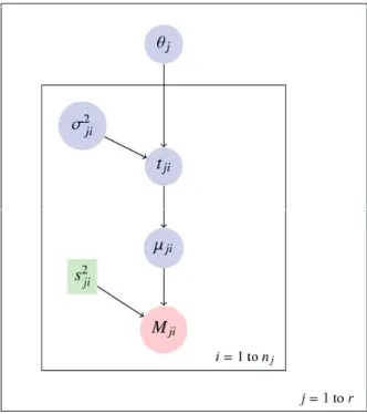
Figure 2:Directed acyclic graph for the hierarchical model of a group of event dates.
assume the independence of the measurements conditionally to the event dates (θ1, . . . , θr)
p(M1, . . . , Mr, θ1, . . . , θr)= p(θ1, . . . , θr) r
∏
j=1
p(Mj|θj),
where p(Mj|θj) is the conditional distribution of Mj givenθj in the hierarchical model defined in
(2.3). Figure 2 summarizes the Bayesian model.
When there is no supplementary information, we assumed that the datesθjare independent and
uniformly distributed on the time interval (study period) T = [Ta, Tb]. This interval is fixed by the
user based on historical or archeological evidences. Consequently, the prior on vectorθ is such that:
p(θ1, . . . , θr)= 1 (Tb− Ta)r r ∏ j=1 1T(θj). (3.1)
Figure 2 describes the overall Bayesian model using a directed acyclic graph. Such a graph de-scribes the dependencies in the joint distribution of the probabilistic model. Each random variable of the model (that is an observation or a parameter) appears as a node in the graph. Any node is conditionally independent of its non-descendants, given its parents. The circles correspond to all ran-dom variables of the model. With the color of the circles, we distinguish between observations (red), parameters (blue) and exogenous variables (green).
We often do not know how a group of event dates can a priori be distributed in a phase. It means that, in our approach, a phase does not respond to a statistical model. From a chronological point of view, all the information is carried by the target event dates themselves. Consequently, we estimate
the beginning and the end of a phase as a measurable application of the parametersθj( j= 1, . . . , r).
Thus the beginning of a phase is estimated by the minimumθ(1)of the r event dates included in the phase
θ(1)= min(θj, j = 1, . . . , r). (3.2)
In the same way, the end of a phase is estimated by the maximumθ(r)of the r event dates included in the phase:
θ(r) = max(θj, j = 1, . . . , r). (3.3)
By the plug-in principle, we estimate the duration of the phase by
τ = θ(r)− θ(1). (3.4)
Considering two phases Pk = {θk,1, . . . , θk,rk}, k = 1, 2, the hiatus between P1and P2is the time
gap between the end of P1and the beginning P2. The hiatus is estimated by: γ = max(θ2,(1)− θ1,(r1), 0
),
(3.5) whereθ2,(1) = min(θ2,1, . . . , θ2,r2) andθ1,(r1) = max(θ1,1, . . . , θ1,r1). Note that the estimateγ takes the
value 0 ifθ1,(r1) ≤ θ2,(1), that corresponds to the absence of hiatus. The conditional distributions of
the parametersθ(1), θ(r), γ, and τ given the observations can be easily derived from the joint posterior distributions of the event dates.
Remark 3. These parameters are estimated knowing the data from the target event dates which are
available in the phase of interest. In particular, a good estimation of the beginning (resp. the end) of a phase requires that the archaeologist has sampled artifacts belonging to target events which are very near to this beginning (resp. this end).
These estimates are valid whatever the prior on the event dates are. Precision on the estimation of these parameters can be gained if it is possible to add supplementary information on the target event dates within the study period T . For instance some temporal orders induce some restrictions on the support of the distribution.
Different prior on dates θjcan be defined according to the following circumstances:
• Relative dating based on stratigraphy as defined in Harris (1989) and Desachy (2005, 2008), can im-ply antero-posteriority relationships between target datesθj. This can also imply antero-posteriority
relationships between groups of datesθj, these groups defining different phases.
• We can have some prior information about the maximal duration of a group of target events. • We can also have some prior information about the minimal temporal hiatus between two groups
of target events.
It has been demonstrated that these types of supplementary prior information can significantly improve chronometric dates (see initial works of Naylor and Smith (1988); Buck et al. (1991, 1992, 1994, 1996) and Christen (1994)). In the next three subsections, we discuss each of these prior information in the framework of the target event date model. Our modeling approach is very soft because all relationships operate directly onto the target event datesθj. As a consequence, in a global
modeling project, different phasing systems (multiphasing) can be defined based on different criteria and so a phasing system can intersect another phasing system: for example a ceramic phasing can intersect a lithic phasing in the sense that some target events can belong to two or several phases. Such a constraints network, when available, can significantly contribute to improve the precision of the estimates.
3.2. Prior information on temporal order
Target events or phases (groups) of target events can have to check order relationships. This order can be defined in different ways: by the stratigraphic relationship (physical relationship observed in the field) or by stylistic, technical, architectural, . . . , criteria which may be a priori known. Thus, the constraint of succession is equivalent to a hiatus of unknown amplitude put between event dates or groups (phases) of event dates.
If we consider a stratigraphic sequence composed of target events, the prior on vectorθ becomes:
p(θ1, . . . , θr)∝ 1 (Tb− Ta)r 1C(θ1, . . . , θr) (3.6) with C= S ∩ Trand • Tr= [T
a, Tb]rthe support which defines the study period,
• S = the group of r-uplets event dates θjwhich respect total or partial order relationships.
We can also consider two groups of target events, Pk = {θk,1, . . . , θk,rk}, k = 1, 2, containing rk
event dates such that all the dates of P1are before all the dates of P2. The following equations should be verified by all events included in both phases.
∀ j ∈ {1, . . . , r1}, ∀l ∈ {1, . . . , r2}, θ1, j< θ2,l or
max(θ1, j, j = 1, . . . , r1)< min(θ2,l, l = 1, . . . , r2) or
min(θ2,l, l = 1, . . . , r2)− max(θ1, j, j = 1, . . . , r1)> 0. (3.7) The r-uplets event datesθjwill then have to check total or partial stratigraphic constraints and
also to satisfy the inequality (3.7) between event dates of the two phases. We can see that a succes-sion constraint between phases operates in the same mathematical way as for a set of stratigraphic constraints put between all individual target events.
Remark 4. Estimating the date of a target event needs to incorporate several dates (Ed), otherwise
the event date modeling will not yield a better posterior information. However, it is possible to nest only one date per target event provided that the group of events is constrained by temporal order.
It is not rare to encounter dating results which contradict the stratigraphic order. This situation of stratigraphic inversion often occurs when some artifact movements are provoked for example by bioturbations or establishment of backfill soils. The target event date model makes it possible to manage such situations thanks to the individual variancesσ2i which automatically penalize the dates that are inconsistent with the stratigraphic order as illustrated in Section 5.2.
3.3. Prior information about the duration
Prior information can be included on the duration of a phase, that is on a group of target events. We can impose a maximal durationτ0. This means that all the event datesθj( j = 1, . . . , r) in the phase
have to verify the constraint of duration according to the following equation:
max(θj, j = 1, . . . , r) − min(θj, j = 1, . . . , r) ≤ τ0. (3.8) The r-uplets event datesθjwill have to check total or partial stratigraphic constraints and also to
satisfy the inequality 3.8 between event dates in the phase. This means that any r-upletθjsampled
during the Markov chain Monte Carlo (MCMC) process has a duration of at the mostτ0.
3.4. Prior information about the amplitude of a hiatus
Prior information about a hiatusγ between two phases Pk= {θk,1, . . . , θk,rk}, k = 1, 2, may be available.
Hence we can impose that the amplitude of the hiatus is higher than a known valueγ0 > 0. All the event dates of phase P1and phase P2have to verify the following constraint :
min(θ2,l, l = 1, . . . , r2)− max(θ1 j, j = 1, . . . , r1)≥ γ0. (3.9) The event dates will have to check total or partial stratigraphic constraints and also to satisfy the inequality (3.9). This means that any r-uplet θ1, j from phase P1 and sampled during the MCMC process is separated by a time span of at leastγ0 from the r-upletθ2,lof the next phase. Note that it is obviously not possible to impose a hiatus between two phases when a same event belongs to these two phases.
3.5. Prior information about known event dates: the bounds
Bounds, such as historical dates, TPQ or TAQ, may also be introduced in order to constrain one or several event datesθj. If we consider a set of r events assumed to happen after a special event with
true calendar date B such that
B< (θ1, . . . , θr).
This condition must be included in the set of constraints that define the support of the prior distribution of the event dates.
The bound can be also defined with an uncertainty, i.e., B ∈ [Ba, Bb] ⊂ [Ta, Tb], and so it is
included in the set of the parameters. The prior density of the event dates can then be written as:
p(θ1, . . . , θr, B) = p(θ1, . . . , θr|B)p(B), where p(θ1, . . . , θr|B) = 1 (Tb− B)r r ∏ j=1 1[B,Tb](θj) and p(B)= 1 Bb− Ba 1[Ba,Bb](B).
It is important to note that the introduction of bounds B in a global model composed of groups (phases) of event dates must remain consistent with other constraints of temporal order, of duration or of hiatus described in previous sections.
4. Discussion on date prior probabilities
In this section we discuss the question of the specification of the prior on the event datesθj. When
there is no supplementary information, it may seem natural to assume that the datesθjare
indepen-dent and uniformly distributed on the time interval (study period) T = [Ta, Tb]. However, from an
archaeological point of view, it may seem more natural to assert that the span∆ = max(θj)− min(θj)
has a uniform prior distribution We can see that this assumption is not checked when starting from the prior density (3.1). After an appropriate change of variable and letting R= Tb− Ta, we can determine
the density of the span according to the number of dates r and regardless their order:
p(∆) = r(r− 1)
Rr (R− ∆)∆
r−2 (4.1)
A span of 2∆ is favored over a span of ∆ by a factor of about ∆r−2when∆ ≪ R (spreading tendency
when r becomes large). This behavior occurs regardless of the order between dates.
Naylor and Smith (1988), Buck et al. (1992, 1996), Christen (1994), Nicholls and Jones (2002) propose a specific phase modeling to avoid this spreading bias. We study the properties of this mod-eling implemented in BCal and OxCal software. The Naylor-Smith-Buck-Christen (NSBC) prior is defined for a group of event dates which are placed between two additional hyperparametersα and β in the Bayesian hierarchical structure. These hyperparametersα and β represent boundaries where α is the beginning andβ the end of the group of events called Phase. The dates θj are assumed to be
independent conditionally to these two boundaries. Then, the prior density on vectorθ becomes:
p(θ1, . . . , θr|α, β) =
1
(β − α)r1[α,β]r(θ1, . . . , θr). (4.2)
In the absence of supplementary information, a non informative prior density is assigned toα and β:
p(α, β) = 2
(Tb− Ta)2.1
P(α, β) (4.3)
with P= {(α, β) | Ta≤ α ≤ β ≤ Tb}. The pairs (α, β) are uniformly distributed on the triangle P.
From these hypotheses, it is possible to calculate the prior joint probability density of the event dates (θ1, . . . , θr). This is carried out by integration againstα and β between the two limits Taand Tb.
For 2 (ordered or non ordered) event datesθ1, θ2, we obtain:
p(θ1, θ2)= ∫ p(θ1, θ2|α, β) · p(α, β) dα dβ = ∫ 1 (β − α)2 · 1[α,β](θ1)· 1[α,β](θ2) 2 (Tb− Ta)2 · 1[Ta≤α≤β≤Tb](α, β). dα dβ = 2 (Tb− Ta)2 ∫ min(θ1,θ2) Ta ∫ Tb max(θ1,θ2) 1 (β − α)2dβ dα = 2 (Tb− Ta)2 ∫ min(θ1,θ2) Ta [ 1 max(θ1, θ2)− α − 1 Tb− α ] dα. Finally, we have: p(θ1, θ2)= 4 (Tb− Ta)2
[− ln(max(θ1, θ2)− min(θ1, θ2))+ ln(Tb− min(θ1, θ2))
Figure 3: “NSBC” phase model: prior joint density on two (non ordered) event datesθ1 andθ2 between two
boundariesα and β and after integration against α and β: a concentration effect appears around values θ1 = θ2.
NSBC= Naylor-Smith-Buck-Christen.
The joint probability density for r (ordered or non ordered) event dates (θj, j = 1, . . . , r) with
r≥ 3, is obtained by following the same integration process: p(θ1, . . . , θr)= 2 r! (r− 1)(r − 2)(Tb− Ta)2 ( 1 [θ(r)− θ(1)]r−2 − 1 [Tb− θ(1)]r−2 − 1 [θ(r)− Ta]r−2 + 1 [Tb− Ta]r−2 ) 1[Ta,Tb]2(θ(1), θ(r)), (4.5)
whereθ(r)= max(θj, j = 1, . . . , r) and θ(1)= min(θj, j = 1, . . . , r).
Equations (4.4) and (4.5) show that the priors (4.2) and (4.3) provoke a strong concentration effect of the datesθjas illustrated in Figure 3 which is calculated for two event dates with formula (4.4). The
region of high probability of (θ1, θ2) is concentrated around the first diagonal (θ1= θ2). In conclusion, the NSBC prior clearly favors the fact that dates (θ1, . . . , θr) become near each other. This property of
the phase can be compared with the assumption of contemporaneity imposed on the dates in the event model.
Starting from the prior densities (4.4) and (4.5), and after an appropriate change of variable, we can also determine the density of the span∆ = max(θj, j = 1, . . . , r)−min(θj, j = 1, . . . , r), according
to the number of dates r. Letting R= Tb− Ta, we obtain:
r= 2 : p(∆) = 4 R2[(R+ ∆)(ln(R) − ln(∆)) + 2(∆ − R))] , (4.6) r= 3 : p(∆) = 6 R2 [ (R− ∆) ( 1+∆ R ) + 2∆(ln(∆) − ln(R)) ] , (4.7) r≥ 4 : p(∆) = 2r (r− 2)R2 [ (R− ∆) ( 1+∆ r−2 Rr−2 ) − 2 r− 2 ( ∆ −∆r−2 Rr−3 )] . (4.8)
These distributions are shown in Figure 4. When r is small (r = 2, 3, 4), the densities are very high for∆ near zero, hence a high concentration effect. When r tends towards infinity, the distribution of∆ tends to p(∆) = (2/R2)(R− ∆). This latter triangular distribution is still maximal when ∆ = 0,
Figure 4:Distributions of the span∆ pour different values of the number r of event dates in a NSBC phase model with: Ta ≤ α ≤ θ1, . . . , θr ≤ β ≤ Tb. When r is small (r= 2, 3, 4), the densities are very high for ∆ near zero,
reflecting a high concentration effect. NSBC = Naylor-Smith-Buck-Christen
and it becomes more and more flat as R increases. Nicholls and Jones (2002) proposed to make the prior distribution on the datesθj uniform by multiplying the prior in (4.3) by R2/{2(R − ∆)} where
min(θj, j = 1, . . . , r) is replaced by α and max(θj, j = 1, . . . , r) by β. This option is implemented in
OxCal when setting UniformSpanPrior=true’ in a modeling project (Bronk Ramsey, 2009a). Instead of looking at span∆, we can look at the variance of the event dates θj, which is more
rep-resentative of their scattering. This variance is proportional to the sequence of the Euclidian distance of the event dates to the straight lineθ1 = θ2 = · · · = θr in the space of dimension r and therefore
it gives a good way to characterize the scattering of the dates. We observe that this distance remains near zero whatever the number r of event dates. Figure 5 shows an evaluation of the dispersion of the dates through the density of the statistic
1 r r ∑ i=1 θi− 1 r r ∑ j=1 θj 2 (4.9)
obtained with r= 10. Conditionally to (α, β), the event dates are uniformly sampled between α and β and the distribution of (α, β) is given by
p(α) = 2(Tb− α) (Tb− Ta)2 , p(β|α) = 1 (Tb− α) 1[α,Tb](β).
Note that we simulate a sample from the prior distribution of (α, β) as: 1. Generate u∼ Uniform(0, 1),
Figure 5:Alternate view of the concentration effect in the NSBC phase model: distribution of (4.9) for r = 10 event dates with: Ta= 0 ≤ α ≤ θ1, . . . , θ10≤ β ≤ 100 = Tb. NSBC= Naylor-Smith-Buck-Christen
(a) NSBC phase model (b) Event date model
Figure 6:Posterior distribution of parameters. NSBC= Naylor-Smith-Buck-Christen
2. Takeα = Tb− R
√ 1− u, 3. Generateβ ∼ Uniform(α, Tb).
The same result is obtained whatever the partial or total order of the event dates.
The concentration effect is particularly visible when considering dates with different uncertainties. In this case, the posterior results forα and β are attracted by the most precise dates.
Our result shows that the prior on event datesθjgiven by formulas (4.4) and (4.5) does not give an
ideal solution for the specification of the prior density on datesθj. It allows the correction of the date
spreading bias when the uncertainties on the dates are of the same amplitude, but it can generate some undesirable concentration effect when the uncertainties are different from each other. This behavior is illustrated in the following example.
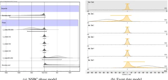
Example 1. Synthetic data in NSBC phase
We consider a phase with 5 non ordered Gaussian dates: 3 dates 0±30 AD, 1 date −500±200 AD and 1 date+500±200 AD. We can see in Figure 6(a) that the posterior densities for α and β calculated with the OxCal program are close to the precise dates 0± 30, a result predicted by formula (4.4). Of
note is that the agreement index A given by OxCal are low and produce a warning to prevent from an over-interpretation of the result. Figure 3(b) shows the result obtained with ChronoModel program when the five dates are nested in the event date model. We observe that the NSBC result tends to behave like the event date model in the sense that it favors the contemporaneity of the dates.
In conclusion, the specification of an appropriate prior on target event dates remains an open question. We showed that the NSBC phase model favors, in an underlying way, the concentration of the event dates in a phase. We also showed that the uniform prior favors spreading dates, especially when temporal order constraints act.
5. Simulations
In this section, Monte Carlo experiments are done to illustrate the performance of the proposed model on simulated samples. All the simulations are done using the R package ArchaeoChron (Philippe and Vibet, 2017c).
5.1. The target event model
To illustrate the properties of the event date modeling, especially its robustness, we simulate sample of measurements Miwith outliers using a mixture with two Gaussian components:
(1− q)N(0, 1) + qN(µ, 1). (5.1)
The date of the target event is 0, and q represents the proportion of outliers. We compare the event target model with
• the r-combine model (Remark 1). • the t-outlier model (Section 2.2).
We assume that all the measurements have the same calibration curve, this condition is required for the r-combine model. We take g(x) = x and σg = 0. The time range (study period) T is set equal to
[−20, 20], Figures 7 and 8 represent the boxplot of the Bayes estimates evaluated on 500 independent replications. This confirms that the r-combine model is not robust to outliers. For q= 0 (no outlier) the three models gives the same results, we do not observe a significant difference in terms of accuracy. The target event model and the t-outlier model behave similarly and provide robust statistical methods. Indeed, for q< 5% the presence of outliers has practically no influence on the target date result in the sense that the boxplots stay centered around the true value.
The lengths of the boxplots also indicate that the loss of accuracy if less important for event model than the t-outlier model. To understand the robustness of the target event model, we represent in Figure 8 the boxplot of the Bayes estimate of the individual varianceσ2i. We compare the values of this parameter when the date tiof the dated event is an outlier or not. Recall that the date ti is an
outlier when it is not contemporaneous of the date θ. Figure 8 shows that the individual standard deviation takes large values for the outlier. This penalizes the contribution of the observation on the estimation of the date, leading to robust procedure. Moreover regardless to the proportion of outliers, the behavior is the same.
5.2. Chronological model
In this part, we illustrate the behavior of our chronological model in presence of stratigraphic inver-sion. We want to date target events that satisfy stratigraphy constraintsθ1 < θ2 < · · · < θ10. To
0 % 5 % 10 % 16 % −0.2 0.0 0.2 0.4 0.6 0.8 1.0 event model 0 % 5 % 10 % 16 % −0.2 0.0 0.2 0.4 0.6 0.8 1.0 outlier model 0 % 5 % 10 % 16 % −0.2 0.0 0.2 0.4 0.6 0.8 1.0 rcombine
Figure 7:Evolution of the Bayes estimate ofθ (the date of the target event (2.5)) as a function of the proportion
qof outlier for three Bayesian models. The number of replication is 500. The data are simulated from (5.1) with µ = 5 and the sample size is 100. The hyperparameter in (2.12) are fixed σδ= 10 and p = 5%.
0 % 5 % 10 % 16 % 1.0 1.5 2.0 2.5 −a− 1 % 5 % 9 % 14 % 19 % 1 2 3 4 5 6 −b−
Figure 8:Evolution of the Bayes estimator ofσiin (2.4). Comparison between a non- outlier (a) and an outlier
(b) as function of the proportion of outlier q. The parameters are the same as in Figure 7.
compare our model with the t-outlier model, we construct target event containing only one dated event. We denote t1, t2, . . . , t10the dates of dated event. To evaluate the robustness of event model, we assume that the date t5creates a stratigraphic inversion. We takeθi= tifor all i, 5 and t5> θ5.
We simulate sample of 10 measurements such that the true dates satisfy the condition t1 < t2 < · · · < t10. Then, we shift the observation associated with the date t5to create the stratigraphic inversion in the observations. The prior information on the dates of target events isθ1 < · · · < θnwhile this
constraints is imposed on the dates t1 < t2 < · · · < t10for the t-outlier model. The time range (study period) T is set equal to [−10, 100]. Figures 9 and 10 compares our model with the t-outlier model.
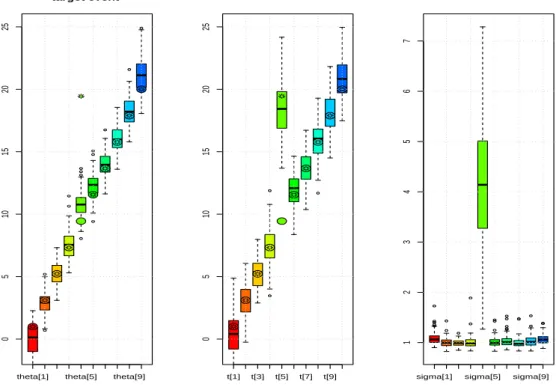
Figure 9 gives the results for the target event model. The value of t5 appears as an outlier, as shown by the high values of the standard deviationσ5 (Figure 9). The estimations of t5are centered around the true value since the stratigraphic constraints is not imposed to the parameters ti. Due to
theta[1] theta[5] theta[9] 0 5 10 15 20 25 target event ● ● ● ● ● ● ● ● ● ● t[1] t[3] t[5] t[7] t[9] 0 5 10 15 20 25 ● ● ● ● ● ● ● ● ● ●
sigma[1] sigma[5] sigma[9]
1 2 3 4 5 6 7
Figure 9: Boxplot of the Bayes estimates of parameters (θi, ti, σi)i=1,...,10in the Target event model (2.3). The
circles (resp. stars ) indicate the true values of the datesθi(resp ti). The number of replication is equal to 500.
the stratigraphic constraint, the Bayes estimate ofθ5is far from the true values of t5. But this outlier does not disturb the estimation of the rest of the sequence. For all the other dates the stratigraphic constraints onθibring prior information and make more precise the target datesθithan the dates ti.
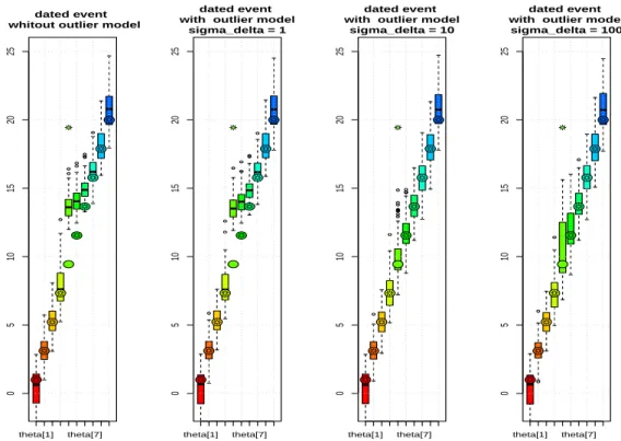
Figure 10 gives the results of the t-type outlier model is applied to the same datasets for different values of the parameterσδ. Whenσδ = 0, the outlier are not taken into account in the model. For a good choice of the parameterσδ(here 10), the performance of the t-outlier model is quite similar to the target event model. But Figure 10 shows that the t-type outlier model is very sensitive to the choice of its hyperparameter. The lack of an adaptive choice for this parameter is the main drawback of this approach.
6. Applications
The model is implemented in the cross-platform application ChronoModel which is free and open source software (Lanos et al., 2016). Features of the application are described in detail in (Vibet
et al., 2016): graphical user interface for importing data and modeling construction, MCMC options
and controls, graphical and numerical results. Different graphical tools are implemented to assess the convergence of the MCMC: the history plot, the autocorrelation function, the acceptance rate of Metropolis-Hastings algorithms (details in Appendix) The user can adjust the length of burn-in, the maximum number of iterations for adaptation and for acquisition, and the thinning rate (Vibet et al., 2016).
theta[1] theta[7] 0 5 10 15 20 25 ● ● ● ● ● ● ● ● ● ● dated event whitout outlier model
theta[1] theta[7] 0 5 10 15 20 25 ● ● ● ● ● ● ● ● ● ● dated event with outlier model
sigma_delta = 1 theta[1] theta[7] 0 5 10 15 20 25 ● ● ● ● ● ● ● ● ● ● dated event with outlier model
sigma_delta = 10 theta[1] theta[7] 0 5 10 15 20 25 ● ● ● ● ● ● ● ● ● ● dated event with outlier model sigma_delta = 100
Figure 10:Boxplot of the Bayes estimates of tifor the t-outlier model with different values of the hyperparameter
in (2.12) : σδvaries and p= 5%. The simulated sample are the same as in Figure 9 The circles (resp. stars ) indicate the true values of the datesθi(resp ti).
6.1. Lezoux (Auvergne, France): last firing of a potter’s kiln
The aim is to date the last firing of a medieval potter’s kiln recovered at the Maison-de-Retraite-Publique site (Mennessier-Jouannet et al., 1995), in Lezoux (Auvergne, France). The target event corresponds to the last firing of the kiln that corresponds to the last use of the kiln (i.e. behavioral event, according to Dean (1978)). Some events relevant to this target event are dated by three chrono-metric techniques: archaeomagnetism (AM), thermoluminescence (TL) and radiocarbon (14C). AM and TL dates are determined from baked clay and 14C date from charcoals of trees assumed to be felled at the same time as the last firing.
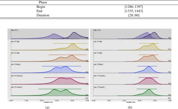
The observations are composed of 3 TL dates (CLER 202a, 202b, 203), 2 AM dates (inclination, declination), and 1 radiocarbon date (Ly-5212) As the kiln belongs to the historical period, the prior time range T is set equal to [−1000, 2000]. Posterior densities ti (in color) obtained are greatly
shrunken compared to individual calibrated densities (in black line), especially for archaeomagnetic and TL dates. The target date gives a 95% highest posterior density (HPD) interval equal to [574, 885] AD. Some of the posterior densities for standard deviationsσi(Figure 12) are spread. This comes
from the multimodality of AM calibrated dates obtained with inclination (Inc) and declination (Dec). More generally, the parameterσitakes larger values when the associated date tiis a possible outlier
Figure 11: Lezoux. [white background ] Posterior densities of ti and individual posterior calibrated densities
(black line) obtained for TL dates, for14C dates and for AM dates. [gray background ] Posterior density for
eventθ. The bar above the density represents the shorter 95% posterior probability interval (credibility interval). The vertical lines, delimiting the colored area under the density curve, indicate the endpoints of the 95% highest
posterior density (HPD) region.
Figure 12:Lezoux. Posterior densities obtained for standard deviationsσi.
6.2. Duration constraint: household cluster from Malpa´ıs Prieto site (Michoac ´an State, Mexico)
In some favorable archaeological contexts, it is possible to get information about the duration of a phase. It is the case here with a household cluster excavated on the Malpa´ıs Prieto site (Michoac´an State, Mexico), in the framework of the archaeological project Uacusecha (Pereira et al., 2016). The archaeological artifacts are typical of a chrono-ceramic phase dated to the period 1200–1450 AD, so the prior time range (study period) T can be set equal to this interval. Five radiocarbon ages have been obtained from burials (bone samples) and a midden (charcoal samples). Looking at the individual calibrated radiocarbon dates, which appear to be consistent between them (no outliers), the overall date range for the occupation is between 1276 and 1443 AD (at 95% confidence level). Each radiocarbon date corresponds to one target event and these events allow the estimation of the beginning and the end of the household cluster phase to which they belong to (Figure 13(a)). This
Table 1:95% highest posterior density region for estimating the phase (begin/end/duration)
Phase
Begin [1209; 1355]
End [1372; 1450]
Duration [48; 211]
Table 2:95% highest posterior density regions for estimating the phase (begin/end/duration) (τ0= 60)
Phase
Begin [1286; 1397]
End [1335; 1443]
Duration [28; 60]
(a) (b)
Figure 13: Malpa´ıs Prieto, without informative constraint (a) and with constraint of maximal durationτ0 = 60
(b). Each picture provides the posterior densities for event datesθj[gray background] and the posterior densities
for beginning and end of the phase [dark gray background]. The bar above the density represents the shorter 95% posterior probability interval (credibility interval).
modeling with only one date per target event and without any stratigraphic or duration constraints gives large 95% HPD intervals for beginning and end estimates (Table 1).
The simple modeling does not allow to significantly improve the prior archaeological information. To do this, various archaeological evidences can better constrain the occupation duration: stratigraphic evidence, accumulation processes of the occupation remains, and durability of the partly perishable architecture. In this example, these information indicate that the occupation has hardly exceeded one century, the most plausible estimation being between 60 and 90 years. As a trial, we consider that the phase duration cannot exceedτ0 = 60 years. Applying this constraint during the MCMC sampling according to (3.8), we obtain the following results (Figure 13(b)) (Table 2).
Posterior densities of the target event datesθj in Figure 13(b) are shrunken compared with the
unconstrained modeling. Moreover, this modeling tends to favor the recent part of the study period, by mitigating the bimodal shape of the individual calibrated dates.
7. Conclusion
The Bayesian event date model aims to estimate the dateθ of a target event from the combination of individual dates ticoming from relevant dated events. This model has a hierarchical structure that
makes it possible to distinguish between target event dateθ (the date of interest for the archaeologist) and dates tiof events (artifacts) dated by chronometric methods, typo-chronology or historical
docu-ments. One assumes that these artifacts are all contemporaneous and relevant to the date of the target event. The dates can be affected by irreducible errors, hence the possible presence of outliers. To take into account these errors, the discrepancy between dates tiand target dateθ is modeled by an
individ-ual varianceσ2i that allows the model to be robust to outliers in the sense that individual variances act as outlier penalization. The posterior distribution of the varianceσ2i indicates if an observation is an outlier or not. Thanks to this modeling, it is not necessary to discard outliers because the correspond-ing high valuesσ2i will automatically penalize the contributions to the event date estimation. This model also does not require additional exogenous or hyperparameters. The only parameter involved in prior shrinkage, s2
0 , comes uniquely from the data analysis via the individual calibration process. The approach is therefore adapted to very different datasets. The good robustness properties of the event date model are paid with less precision in the dates. However, this loss of precision is compen-sated by a better reliability of the chronology. The event model constitutes the basic element in our chronological modeling approach. Dating data are nested within target event dates (with or without stratigraphic constraints between them) which may be nested into phases (with or without succession constraints between them). Succession constraint, maximal duration and/or minimal hiatus can be put on the event dates in the phases.
Appendix A: MCMC computation Algorithms
The posterior distributions of the parameter of interestθ and of other related parameters tiandσican
not be obtained explicitly. It is necessary to implement a computational method to approximate the posterior distributions, their quantiles, the Bayes estimates and the highest posterior density (HPD) regions. We adopt a Markov chain Monte Carlo (MCMC) algorithm known as the Metropolis-within-Gibbs strategy because the full conditionals cannot be simulated by standard random generators. For each parameter, the full conditional distribution is proportional to (2.3). Details on the algorithms used are given in (Lanos and Philippe, 2017).
Here we give a more detailed insight on the way to estimate the date ti, which is defined on the set
R due to the random effect model chosen in (2.2). The full conditional distribution of ti(∀i = 1, . . . , n)
is given by p(ti|•) ∝ 1 Si(ti) exp −1 2S2 i(ti) (Mi− gi(ti))2 exp −1 2σ2 i (ti− θ)2 , (A.1) where S2 i(ti)= s 2 i + σ 2
gi(ti). Symbol• represents the observations and all other parameters according
to equation (2.3).
To estimate the posterior density of ti, we can choose between three MCMC algorithms. In each
case, the support of the proposal density includes the supportR of the target posterior density. • MH-1: A Metropolis-Hastings algorithm where the proposal is the prior distribution of the
param-eter. This method is recommended when no calibration is needed, namely for TL/OSL, Gaussian measurements or typo-chronological references.
• MH-2: A Metropolis-Hastings algorithm where the proposal is an adaptive Gaussian random walk. This method is adapted when the density to be approximated is unimodal. The variance of this proposal density is adapted during the process.
• MH-3: Metropolis-Hastings algorithm where the proposal mimics the individual calibration den-sity. This method is adapted for multimodal densities, such as calibrated measurements.
We are frequently confronted with multimodal target distributions as, for instance, in archaeomag-netic dating (Example 6.1). In this case, algorithms MH-1 and MH-2 are not well adapted to ensure a good mixing of the Markov chain. Consequently, an alternative is to choose the MH-3 algorithm with a proposal distribution that mimics the individual calibration density defined in (2.7). In order to ensure the convergence of MCMC algorithm, the support of the proposal must beR. Thus we can consider a mixture having a gaussian component. This component ensures that the whole support is visited. So we take as proposal :
λC + (1 − λ)N ( 0,1 4(Tb− Ta) 2 ) , (A.2)
whereλ is a number fixed close to 1, and the distribution C approximates the individual calibration density. We can choose for instance the empirical measure calculated on the simulated sample from (2.7) or a mixture of uniform distribution:
M ∑ i=1 1 MUniform ([ ˜ti, ˜ti+1 ]), where (˜ti)i=1,...,Mare the ordered values of the simulated sample.
An alternative is to choose the distribution with density 1 C p ∑ i=1 pi(τi)I[τi,τi+1], where C = p ∑ i=1 f (τi)(τi+1− τi),
where (τi)iis a deterministic grid of T and piis the density of individual calibration density (2.7).
Assessing Convergence
Using the packages ArchaeoPhases and coda implemented in R (Philippe and Vibet, 2017b; Plum-mer et al., 2006; R Core Team, 2017), we check the convergence of MCMC samples simulated for different values of the parameters λ in (A.2).
Figures A.1 and A.2 provide graphical tools for the diagnostic of MCMC sampler. We consider the example of Lezoux and only give the result for the parameter of interestθ and the date tdec asso-ciated with the declination measurement in AM dating. Note that the behavior is the same for all the parameters of the model.
Within the Gibbs sampler, the tdecis simulated using MH-3 algorithm, and so the proposal distri-bution depends on the choice of parameterλ in A.2. For three values of λ, Figures A.1 and A.2 show a stationary behavior with good mixing properties. The autocorrelations even at lag 1 are small enough, to provide a good approximation of the posterior distribution and its characteristics (mean/ variance / quantiles). It is also important to note that the results are not sensitive to the value ofλ.
The Gelman diagnostic (evaluated from 5 parallel chains) is equal to 1, and confirms the conver-gence of MCMC samplers.
0 1000 2000 3000 4000 5000 400 500 600 700 800 900 1000 Index 0 1000 2000 3000 4000 5000 400 500 600 700 800 900 1000 Index 0 1000 2000 3000 4000 5000 400 500 600 700 800 900 1000 Index 400 600 800 1000 0.000 0.001 0.002 0.003 0.004 0.005 0.006 0.007 Density 0 5 10 15 20 0.0 0.2 0.4 0.6 0.8 1.0 lag acf
Figure A.1:Lezoux. Diagnostic for MCMC output from posterior distribution of the date of target event. History
plots, autocorrelation and marginal density are represented for different values of λ = 0.99, 0.9, 0.7. MCMC = Markov chain Monte Carlo.
0 1000 2000 3000 4000 5000 500 1500 Index 0 1000 2000 3000 4000 5000 500 1500 Index 0 1000 2000 3000 4000 5000 500 1500 Index
Figure A.2: Lezoux. Diagnostic for MCMC output from posterior distribution of AM-dec date. History plots,
autocorrelation and marginal density are represented for different values of λ = 0.99, 0.9, 0.7. MCMC = Markov chain Monte Carlo.
Acknowledgments
This project is supported by the grant ANR-11-MONU-007 ChronoModel. The authors expressed their gratitude to Gr´egory Pereira (CNRS, UMR ArchAm, University of Paris 1 Panth´eon-Sorbonne) for the exchange of information about the example of Malpa´ıs Prieto site in Mexico.
We also thank Marie Anne Vibet for her very helpful discussions during the preparation of this paper.
References
Bayliss A (2009). Rolling out revolution: using radiocarbon dating in archaeology, Radiocarbon, 51, 123–147.
Bayliss A (2015). Quality in Bayesian chronological models in archaeology, World Archaeology, 47, 677–700.
Bronk Ramsey C (1995). Radiocarbon calibration and analysis of stratigraphy: the OxCal program,
Radiocarbon, 37, 425–430.
Bronk Ramsey C (1998). Probability and dating, Radiocarbon, 40, 461–474.
Bronk Ramsey C (2001). Development of the radiocarbon calibration program OxCal, Radiocarbon, 43, 355–363.
Bronk Ramsey C (2008). Deposition models for chronological records, Quaternary Science Reviews, 27, 42–60.
Bronk Ramsey C (2009a). Bayesian analysis of radiocarbon dates. Radiocarbon, 51, 337–360. Bronk Ramsey C (2009b). Dealing with outliers and offsets in radiocarbon dating, Radiocarbon, 51,
1023–1045.
Bronk Ramsey C, Dee M, Nakagawa T, and Staff R (2010). Developments in the calibration and modelling of radiocarbon dates, Radiocarbon, 52, 953–961.
Bronk Ramsey C and Lee S (2013). Recent and planned developments of the program OxCal,
Radio-carbon, 55, 720–730.
Bronk Ramsey C, van der Plicht J, and Weninger B (2001). Wiggle matching radiocarbon dates,
Radiocarbon, 43, 381–389.
Buck C, Christen J, and James G (1999). BCal: an on-line Bayesian radiocarbon calibration tool,
Internet Archaeology, 7.
Buck C, Kenworthy J, Litton C, and Smith A (1991). Combining archaeological and radiocarbon information: a Bayesian approach to calibration, Antiquity, 65, 808–821.
Buck C, Litton C, and Shennan S (1994). A case study in combining radiocarbon and archaeological information: the early bronze age of St-Veit-Klinglberg, Land Salzburg, Austria, Germania, 72, 427–447.
Buck C, Litton C, and Smith A (1992). Calibration of radiocarbon results pertaining to related ar-chaeological events, Journal of arar-chaeological Science, 19, 497–512.
Buck CE, Higham TFG, and Lowe DJ (2003). Bayesian tools for tephrochronology, The Holocene, 13, 639–647.
Buck CE, Litton CD, and Cavanagh WG (1996). The Bayesian Approach to Interpreting
Archaeolog-ical Data, Chichester, John Wiley and Sons, England.
Christen J (1994). Summarizing a set of radiocarbon determinations: a robust approach, Applied
Statistics, 43, 489–503.
Christen J and P´erez S (2009). A new robust statistical model for radiocarbon data, Radiocarbon, 51, 1047–1059.
Comb`es B and Philippe A (2017). Bayesian analysis of individual and systematic multiplicative errors for estimating ages with stratigraphic constraints in optically stimulated luminescence dating,
Quaternary Geochronology, 39, 24–34.
Dean JS (1978). Independent dating in archaeological analysis, Advances in Archaeological Method
and Theory, 1, 223–255.
Desachy B (2005). Du temps ordonn´e au temps quantifi´e : application d’outils math´ematiques au mod`ele d’analyse stratigraphique d’Edward Harris, Bulletin de la Soci´et´e Pr´ehistorique Fran¸caise,
102, 729–740.
Desachy, B. (2008). De la formalisation du traitement des donn´ees stratigraphiques en arch´eologie
de terrain. Th`ese de doctorat de l’universit´e de Paris 1, Paris, France.
Dye T and Buck C (2015). Archaeological sequence diagrams and Bayesian chronological models.
Journal of Archaeological Science, 1, 1–19.
Gu´erin G, Antoine P, Schmidt E, Goval EDH, Jamet G, Reyss JL, Shao Q, Philippe A, Vibet MA, and Bahain JJ (2017). Chronology of the upper Pleistocene loess sequence of Havrincourt (France) and associated Palaeolithic occupations: a Bayesian approach from Pedostratigraphy, osl, radio-carbon, tl and esr/u-series data. Quaternary Geochronology, 42, 15–30.
Harris E (1989). Principles of Archaeological Stratigraphy. Interdisciplinary Statistics, XIV, 2nd edition. second ed. Academic Press, London.
Lanos P and Philippe A (2017). Hierarchical Bayesian modeling for combining dates in archaeologi-cal context, Journal de la Soci´et´e Fran¸caise de Statistique, 158, 72–88.
Lanos P, Philippe A, Lanos H, and Dufresne P (2016). ChronoModel: Chronological Modelling of
Archaeological Data using Bayesian Statistics. (Version 1.5) http://www.chronomodel.fr
Mennessier-Jouannet C, Bucur I, Evin J, Lanos P, and Miallier D (1995). Convergence de la typologie de c´eramiques et de trois m´ethodes chronom´etriques pour la datation d’un four de potier `a lezoux (puy-de-dˆome), Revue d’Arch´eom´etrie, 19, 37–47.
Naylor JC and Smith AFM (1988). An archaeological inference problem. Journal of the American
Statistical Association, 83, 588–595.
Nicholls G and Jones M (2002). New radiocarbon calibration software, Radiocarbon, 44, 663–674. Niu M, Heaton T, Blackwell P, and Buck C (2013). The Bayesian approach to radiocarbon calibration
curve estimation: the intcal13, marine 13, and shcal13 methodologies. Radiocarbon, 55, 1905– 1922.
Pereira G, Forest M, Jadot E, and Darras V (2016). Ephemeral cities? the longevity of the postclassic tarascan urban sites of zacapu malpas and its consequences on the migration process. In Arnauld, M., Beekmann, C., and Pereira, G., editors, Ancient Mesoamerican Cities: Populations on the
move, page in press. University Press of Colorado, Denver, USA.
Philippe A and Vibet MA (2017a). Analysis of Archaeological Phases using the CRAN Package ArchaeoPhases, preprint hal-01347895.
Philippe A and Vibet MA (2017b). ArchaeoPhases: Post-Processing of the Markov Chain Simulated
by ’ChronoModel’, ’Oxcal’ or ’BCal’. R package version 1.3.
Philippe A and Vibet MA (2017c). ArchaeoChron: Bayesian Modeling of Archaeological
Chronolo-gies. R package version 0.1.
Plummer M, Best N, Cowles K, and Vines K (2006). Coda: Convergence diagnosis and output analysis for MCMC, R News, 6, 7–11.
R Core Team (2017). R: A Language and Environment for Statistical Computing. R Foundation for Statistical Computing, Vienna, Austria.
Vibet, MA, Philippe A, Lanos P, and Dufresne P (2016). ChronoModel v1.5 user’s manual, from: www.chronomodel.fr


![Figure 11: Lezoux. [white background ] Posterior densities of t i and individual posterior calibrated densities (black line) obtained for TL dates, for 14 C dates and for AM dates](https://thumb-eu.123doks.com/thumbv2/123doknet/14743782.577416/22.892.149.749.197.518/background-posterior-densities-individual-posterior-calibrated-densities-obtained.webp)