A multi-platform package for the analysis of intra- and
interspecific trait evolution
Th´eo Gaboriau
*1, F´abio K. Mendes
*2,3, Simon Joly
4,5, Daniele Silvestro
†6,7, and
Nicolas Salamin
†11Department of Computational Biology, University of Lausanne, 1015 Lausanne, Switzerland 2School of Computer Science, The University of Auckland, 1010 Auckland, New Zealand 3School of Biological Sciences, The University of Auckland, 1010 Auckland, New Zealand
4Institut Recherche en Biologie V´eg´etale, Montr´eal, Quebec H1X 2B2, Canada 5Montreal Botanical Garden, Montreal, Quebec, H1X 2B2, Canada 6Department of Biology, University of Fribourg, 1700 Fribourg, Switzerland
7Department of Biological and Environmental Sciences, University of Gothenburg and Global Gothenburg Biodiversity Centre, Gothenburg, Sweden
July 20, 2020
Supplementary information
Well-calibrated validation of JIVE model implementation in
BEAST 2
We verified the correctness of the BEAST 2 implementation of the JIVE model by conducting a well-calibrated validation study. If parameters are inferred using the same priors the data has been simulated under (i.e., no prior misspecification), one should expect the 95% highest posterior densities (HPDs) for each parameter to include the simulated (true) value around 95% of the time. Furthermore, when there is enough signal in the data, there should be some correlation between simulated values and the MCMC-sampled means of their respective posterior distributions.
In our validation procedure, we used the Anolis tree reported in the main text (Fig. 2), and simulated data for 40 individuals per species. We kept species names for consistency, but any other arbitrary names could have been used. We validated three different pairs of models (the priors in JIVE’s Bayesian hierarchical framework) together with the JIVE model, using Brownian motion (BM) as the prior for the species trait log-variances in all three cases, and varying the prior for the species trait means: (i) White noise (WN), (ii) Brownian motion with multiple evolutionary regimes (BMM), and (iii) Ornstein-Uhlenbeck with multiple evolutionary regimes (OUM). The lengths of MCMC chains were 10, 40 and 40 million samples, respectively, with the first 10% of all samples discarded as burn-in in all three cases. We list hyper-priors in table S1.
All parameters exhibited high coverage, as can be seen from the 95% HPD intervals in figures S1 to S9. It was relatively easy to estimate prior parameters of WN and BM models, with the exception of the root value of the log-variances. Under BMM, the two different evolutionary rates proved harder to estimate than when a single rate was used (e.g., in the case of log-variances). This is unsurprising because instead of 16 data points informing a single evolutionary rate, under BMM only 9 and 7 data points informed the first and second rates, respectively. Indeed, the rate
Table S1: JIVE prior distributions used in validation for continuous trait means. The same BM prior was used for trait log-variances, with y0 ∼ U(0.0, 8.02) and σ2 ∼ Γ(α = 1.1, θ = 5.0).
Model Parameter Hyper-prior
WN σ2 Γ(α = 1.1, θ = 5.0) y0 U(0.0, 136.23) BMM σ2 Γ(α = 1.1, θ = 5.0) y0 U(0.0, 136.23) OUM θ U(0.0, 136.23) σ2 Γ(α = 1.1, θ = 5.0) α Γ(α = 1.1, θ = 5.0)
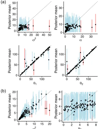
simulated values and their posterior means (Fig. S4). Among OUM prior parameters, there was little correlation between simulated values and posterior means for the evolutionary rate and the strength of the pull toward the “adaptive optima”, α – in many cases, posterior means fell along the prior mean, which indicates identifiability difficulties (Fig. S7). Such unidentifiability issues under the OU model are well-known and have been described in the literature [6; 7; 3].
In all three cases, JIVE parameters (Figs. S2, S3, S5, S6, S8, S9) showed high correlation be-tween simulated values and their respective posterior means. We noted that species means were harder to sample than species log-variances, especially when the priors on means were BMM and OUM. This was expected given the increased complexity of those two models relative to WN, and the fact that the amount of data remained constant. Because some of BMM and OUM prior parameters were hard to estimate, often being sampled directly from their hyperpriors, the BMM and OUM priors were then more likely to be misspecified (in terms of their parameter values) for their respective JIVE parameters, in turn making the estimation of JIVE parameters more difficult. JIVE-related classes are implemented in BEAST 2’s contraband package, which has not yet been officially released (manuscript in preparation). The code is nonetheless publicly available in https://github.com/fkmendes/contraband.
Analysis of
Anolis data set using BEAST 2
We also analyzed the Anolis data set with our BEAST 2 implementation of the JIVE model, using the best combination of prior models (BM for trait means, OUM for trait log-variances; or mBM-vOUM, see main text), and the same hyperprior distributions employed by the analyses conducted in R. Because our model is highly parameterized, for the sake of brevity we point the reader to the BEAST 2 control (.xml) file accompanying this study for the full list of utilized priors (but see above and below for some of the priors we used). The key difference between this analysis and the one reported in the main text is that here we jointly estimate the phylogeny (topology and divergence times), the mapping of evolutionary regimes for the trait log-variances (θ regimes under the OUM model), and all prior and JIVE parameters. We employed a local morphological clock that is a sub-case of the random local clock proposed by [4], in which the number of shifts in evolutionary regimes is fixed, and the locations of the shifts are sampled. For the purposes of the Anolis example, we fixed the number of shifts to one.
Sequences for the 16 Anolis species were obtained from the literature, and consisted of 48 loci (16S, COI, ND2, RAG1 from [13], and a concatenated block of 46 genes from [1]; we did not use the ECEL1 gene alignment from [13] as only one species was represented in it). We applied the same uncorrelated log-normal relaxed molecular clock model to all gene partitions, but let the partitions have their own substitution model parameters (under HKY + Γ; [11]). As in [1], we concatenated all loci, allowing them to share the same phylogeny, which was constrained to have both “Cuba” and “Hispaniola” clades. We were not aware of any fossil calibration points for the internal nodes of our phylogeny, so we used the posterior intervals from [13] and a calibrated birth-death tree prior [5]. More specifically, we set uniform priors for the root, “Cuba” and “His-paniola” clades from minimum and maximum values of (36, 52), (22, 36), and (18, 30), respectively. Note that here we do not attempt to improve on the trees in [13; 1]. Our data set is considerably sub-sampled (16 out of 191 species descending from the most recent common ancestor of the “Cuba” and “Hispaniola” clades), and our goal is merely to demonstrate how this implementation
Four independent MCMC chains were run for 50 million generations sampling every 25,000, and discarding the first 10% as burn-in. All chains converged with average parameter effective sample sizes greater than 1,000, yielding similar posterior estimates. Results were largely con-cordant with those from the R implementation reported in the main text. Within “Cuba” and “Hispaniola”, we recovered the same phylogenetic relationships reported in [13] (and used in the JIVE R-implementation analyses), with high node support values (Fig. S12). Branches inside “Hispaniola” also exhibited higher posterior estimates of θ for trait log-variances (Fig. 5 in main text) than branches in “Cuba”.
In our BEAST 2 analysis, not only did we sample the phylogeny, but also the mapping of θ evolutionary regimes for trait log-variances. The latter was done by employing a random local (morphological) clock [4] that allows every branch of the tree to have its own evolutionary regime in any given generation of the MCMC chain. Under this model, a binary indicator variable δ of length (2N − 2) (where N is the number of species in the tree) determines how evolutionary regimes are distributed among tree branches. A node i where δi = 0inherits the regime of its parent node, and passes that regime down to its children until a child j has δj = 1, or until a leaf child is reached. δi = 1indicates node i has undergone an evolutionary regime shift at the root-end of its subtroot-ending branch, in which case a new regime value is assigned to node i and passed down to node i’s descendants again until one of the descendants j is a leaf node, or δj = 1. We point the interested reader to the original work [4] describing our implementation of the random local clock.
To our knowledge, this is the first time a morphological clock is used to estimate both the location and number of regime shifts and the species tree simultaneously, while accounting for uncertainty. Our morphological clock is general and can readily be used with both BM and OU models (in the former, regimes are evolutionary rates; in the latter, adaptive optima). Previously proposed Bayesian morphological clocks differ from ours in that they (or some of them) (i) em-ploy reversible-jump MCMC (rjMCMC) rather than Bayesian stochastic search variable selection (BSSVS), (ii) were originally aimed at either BM [14; 9] or OU [15], (iii) assume a single regime
shift anywhere on a branch [14], (iv) do not allow for homoplasy [9; 15], and (v) cannot be used while estimating the species tree itself.
We must note that many other frequentist morphological clocks exist, but are very different in nature and can hardly be compared to ours. First, they take the phylogeny as data and do not account for phylogenetic uncertainty (or uncertainty around any parameter, for that matter). For this reason, running times like 45 minutes [2] and 20 hours [10] on a single, fixed 256-taxon tree are acceptable (such times are obviously prohibitive in a Bayesian analysis). Some frequentist clock models are so complex and different, in fact, that they do not bare any visible mathematical or technical resemblance to our implementation. The most extreme example is the model assumed by the “phylogenetic EM” method, which employs an expectation-maximization algorithm after simplifying an OU process to achieve between-trait independence, and after re-scaling the species tree so OU is equivalent to BM; furthermore, this model has to condition on α, so user-specified regime shift numbers are evaluated across a grid of α values – after which the method finally decides on the best by using a likelihood penalization strategy (and we note this is all done on a fixed ultrametric species tree, while not allowing for homoplasy). A few similarities with fre-quentist morphological clocks exist, however, and include assuming (i) sparsity in regime shifts [10; 2], (ii) shifts occur at the root-end of branches [10; 2], and (iii) homoplasy (i.e., convergence; 8; 10).
Our inference of regime shift locations is shown in figure S12. Nodes are colored according to the mean posterior probabilities of their respective δ’s. Interestingly, shifts were more commonly inferred on branches leading to leaf nodes – namely, A. ophiolepis, A. cybotes, and A. strahmi. (Note that we fix the number of shifts in evolutionary regimes to one, meaning that in any gen-eration of the MCMC chain, only a single node is affected by a shift). This placement of shifts is in agreement with these three species having the lowest sample log-variances in “Hispaniola”, and the highest two sample log-variances in “Cuba”, respectively (Fig. 5, main text). In addition, it also reflects the fact that “vOU” (Ornstein-Uhlenbeck with a single adaptive optimum) was an equally good prior model for species trait log-variances as “vOUM”. In other words, although the
difference between trait log-variances of “Hispaniola” and “Cuba” was visible (Fig. 4, main text), it was not marked enough so that shifts were inferred to have occurred on branches leading to these clade’s most recent common ancestors. Instead, the intraspecific trait variances of A. ophi-olepis, A. cybotes, and A. strahmi were more phylogenetically contrasting, leading to shifts in θ on the respective terminal branches. We predict that if more evolutionary shifts were allowed, the posterior probabilities of δ for those species would increase, together with the likelihood of models assigning shifts to internal branches such as those separating “Hispaniola” and “Cuba”. Testing such hypotheses and verifying the power of our local morphological clock is nonetheless outside the scope of this study. Our result highlights the difference between testing a priori hy-potheses with model comparison (e.g., as discussed in the main text; [12]), in which the mapping of evolutionary regimes is fixed, to approaches that average over the location of different regimes, as done by our random local clock implementation [4].
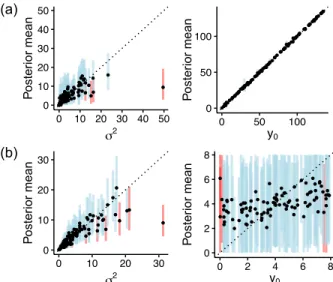
● ● ●●● ● ● ● ● ● ●● ● ● ● ● ● ● ● ● ● ● ● ● ● ● ● ● ● ● ● ● ● ● ● ● ●● ● ● ● ● ● ● ● ● ● ● ● ●● ● ● ● ●● ● ● ● ● ● ●● ● ● ● ● ● ● ● ● ●● ● ● ● ● ● ● ●● ● ● ● ● ● ● ● ● ● ● ● ● ● ●● ● ● ● ● 0 10 20 30 0 10 20 30 σ2 Poste rior mean ● ● ● ● ● ● ● ● ● ● ● ● ● ● ● ● ● ● ● ● ● ● ● ● ● ● ● ● ● ● ● ● ● ● ● ● ● ● ● ● ● ● ● ● ● ● ● ● ● ● ● ● ● ● ● ● ● ● ● ● ● ● ● ● ● ● ● ● ● ● ● ● ● ● ● ● ● ● ● ● ● ● ● ● ● ● ●● ● ● ● ● ● ● ● ● ● ● ● ● 0 2 4 6 8 0 2 4 6 8 y0 Poste rior mean ● ●● ● ● ● ● ● ● ● ● ● ● ● ● ● ● ● ● ● ● ● ●● ● ● ● ● ● ● ● ● ● ● ●●● ● ● ● ● ●● ● ● ●● ● ● ● ● ● ● ● ● ● ● ● ● ● ● ● ● ● ●● ● ● ● ● ●●● ● ● ● ● ● ● ● ● ● ● ● ● ● ● ● ● ● ● ●●● ● ●● ● ● ● 0 10 20 30 40 50 0 10 20 30 40 50 σ2 Poste rior mean ● ● ● ● ● ● ● ● ● ● ● ● ● ● ● ● ● ● ● ● ● ● ●● ● ● ● ● ● ● ● ● ● ● ● ● ● ● ● ● ● ● ● ● ● ● ● ● ●● ● ● ● ● ● ● ● ● ● ● ● ● ● ● ● ● ● ● ● ● ● ● ● ● ● ● ● ● ● ● ● ● ● ● ● ● ● ● ● ● ● ● ● ● ● ● ● ● ● ● 0 50 100 0 50 100 y0 Poste rior mean (b) (a)
Figure S1: Posterior means of prior parameters as a function of their simulated values. (a) WN prior on species means. (b) BM prior on species log-variances. Vertical lines represent the 95% HPD intervals (blue if it includes the true value, red if it does not).
● ● ● ● ● ● ● ● ● ● ● ● ● ● ● ● ● ● ● ● ● ● ●● ● ● ● ● ● ● ● ● ● ● ● ● ● ● ● ● ● ● ● ● ● ● ● ●● ● ● ● ● ● ● ● ● ● ● ● ● ● ● ● ● ● ● ● ● ● ● ● ● ● ● ● ● ● ● ● ● ● ● ● ● ● ● ● ● ● ● ● ● ● ● ● ● ● ● ● 0 50 100 0 50 100 A. ahli Poste rior mean ● ● ● ● ● ● ● ● ● ● ● ● ● ● ● ● ● ● ● ● ● ● ●● ● ● ● ● ● ● ● ● ● ● ●● ● ● ● ● ● ● ● ● ● ● ● ● ● ● ● ● ● ● ● ● ● ● ● ● ● ● ● ● ● ● ●● ● ● ● ● ● ● ● ● ● ● ● ● ● ● ● ● ● ● ● ● ● ● ● ● ● ● ● ● ● ● ● ● 0 50 100 0 50 100 A. allogus Poste rior mean ● ● ● ● ● ● ● ● ● ● ● ● ● ● ● ● ● ● ● ● ● ● ● ● ● ● ● ● ● ● ● ● ● ● ● ● ● ● ● ● ● ● ● ● ● ● ● ●● ● ● ● ● ● ● ● ● ● ● ● ● ● ● ● ● ● ● ● ● ● ● ● ● ● ● ● ● ● ● ● ● ● ● ● ● ● ● ● ● ● ● ● ● ● ● ● ● ● ● ● 0 50 100 0 50 100 A. armouri Poste rior mean ● ● ● ● ● ● ● ● ● ● ● ● ● ● ● ● ● ● ● ● ● ● ●● ● ● ● ● ● ● ● ● ● ● ●● ● ● ● ● ● ● ● ● ● ● ● ● ● ● ● ● ● ● ● ● ● ● ● ● ● ● ● ● ● ● ● ● ● ● ● ● ● ● ● ● ● ● ● ● ● ● ● ● ● ● ● ● ● ● ● ● ● ● ● ● ● ● ● ● 0 50 100 0 50 100 A. cybotes Poste rior mean ● ● ● ● ● ● ● ● ● ● ● ● ● ● ● ● ● ● ● ● ● ● ●● ● ● ● ● ● ● ● ● ● ● ● ● ● ● ● ● ● ● ● ● ● ● ● ● ● ● ● ● ● ● ● ● ● ● ● ● ● ● ● ● ● ● ● ● ● ● ● ● ● ● ● ● ● ● ● ● ● ● ● ●●● ● ● ● ● ● ● ● ● ● ● ● ● ● ● 0 50 100 0 50 100 A. homolechis Poste rior mean ● ● ● ● ● ● ● ● ● ● ● ● ●● ● ● ● ● ● ● ● ● ●● ● ● ● ● ● ● ● ● ● ● ● ● ● ● ● ● ● ● ● ● ● ● ● ● ● ● ● ● ● ● ● ● ● ● ● ● ● ● ● ● ● ● ● ● ● ● ● ● ● ● ● ● ● ● ● ● ● ● ● ● ●● ● ● ● ● ● ● ● ● ● ● ● ● ● ● 0 50 100 0 50 100 A. jubar Poste rior mean ● ● ● ● ● ● ● ● ● ● ● ● ●● ● ● ● ● ● ● ● ● ●● ● ● ● ● ● ● ● ● ● ● ●● ● ● ● ● ● ● ● ● ● ● ● ● ● ● ● ● ● ● ● ● ● ● ● ● ● ● ● ● ● ● ● ● ● ● ● ● ● ● ● ● ● ● ● ● ● ● ● ● ● ● ● ● ● ● ● ● ● ● ● ● ● ● ● ● 0 50 100 0 50 100 A. longitibialis Poste rior mean ● ● ● ● ● ● ● ● ● ● ● ● ● ● ● ● ● ● ● ● ● ● ● ● ● ● ● ● ● ● ● ● ● ● ●● ● ● ● ● ● ● ● ● ● ● ● ●● ● ● ● ● ● ● ● ● ● ● ● ● ● ● ● ● ● ● ● ● ● ● ● ● ● ● ● ● ● ● ● ● ● ● ● ● ● ● ● ● ● ● ● ● ● ● ● ● ● ● ● 0 50 100 0 50 100 A. marcanoi Poste rior mean ● ● ● ● ● ● ● ● ● ● ● ● ●● ● ● ● ● ● ● ● ● ● ● ● ● ● ● ● ● ● ● ● ● ● ● ● ● ● ● ● ● ● ● ● ● ● ● ● ● ● ● ● ● ● ● ● ● ● ● ● ● ● ● ● ● ● ● ● ● ● ● ● ●● ● ● ● ● ● ●● ● ● ● ● ● ● ● ● ● ● ● ● ● ● ● ● ● ● 0 50 100 0 50 100 A. mestrei Poste rior mean ● ● ● ● ● ● ● ● ● ● ● ● ● ● ● ● ● ● ● ● ● ● ●● ● ● ● ● ● ● ● ● ● ● ●● ● ● ● ● ● ● ● ● ● ● ● ●● ● ● ● ● ● ● ● ● ● ● ● ● ● ● ● ● ● ●● ● ● ● ● ● ● ● ● ● ● ● ● ● ● ● ● ● ● ● ● ● ● ● ● ● ● ● ● ● ● ● ● 0 50 100 0 50 100 A. ophiolepis Poste rior mean ● ● ● ● ● ● ● ● ● ● ● ● ● ● ● ● ● ● ● ● ● ● ● ● ● ● ● ● ● ● ● ● ● ● ● ● ● ● ● ● ● ● ● ● ● ● ● ● ● ● ● ● ● ● ● ● ● ● ● ● ● ● ● ● ● ● ● ● ● ● ● ● ● ● ● ● ● ● ● ● ● ● ● ● ● ● ● ● ● ● ● ● ● ● ● ● ● ● ● ● 0 50 100 0 50 100 A. quadriocellifer Poste rior mean ● ● ● ● ● ● ● ● ● ● ● ● ● ● ● ● ● ● ● ● ● ● ● ● ● ● ● ● ● ● ● ● ● ● ●● ● ● ● ● ● ● ● ● ● ● ● ● ● ● ● ● ● ● ● ● ● ● ● ● ● ● ● ● ● ● ● ● ● ● ● ● ● ● ● ● ● ● ● ● ●● ● ● ● ● ● ● ● ● ● ● ● ● ● ● ● ● ● ● 0 50 100 0 50 100 A. rubribarbus Poste rior mean ● ● ● ● ● ● ● ● ● ● ● ● ● ● ● ● ● ● ● ● ● ● ●● ● ● ● ● ● ● ● ● ● ● ● ● ● ● ● ● ● ● ● ● ● ● ● ● ● ● ● ● ● ● ● ● ● ● ● ● ● ● ● ● ● ● ● ● ● ● ● ● ● ●● ● ● ● ● ● ● ● ● ● ● ● ● ● ● ● ● ● ● ● ● ● ● ● ● ● 0 50 100 0 50 100 A. sagrei Poste rior mean ● ● ● ● ● ● ● ● ● ● ● ● ●● ● ● ● ● ● ● ● ● ● ● ● ● ● ● ● ● ● ● ● ● ● ● ● ● ● ● ● ● ● ● ● ● ● ●● ● ● ● ● ● ● ● ● ● ● ● ● ● ● ● ● ● ● ● ● ● ● ● ● ● ● ● ● ● ● ● ● ● ● ● ● ● ● ● ● ● ● ● ● ● ● ● ● ● ● ● 0 50 100 0 50 100 A. shrevei Poste rior mean ● ● ● ● ● ● ● ● ● ● ● ● ● ● ● ● ● ● ● ● ● ● ●● ● ● ● ● ● ● ● ● ● ● ●● ● ● ● ● ● ● ● ● ● ● ● ● ●● ● ● ● ● ● ● ● ● ● ● ● ● ● ● ● ● ● ● ● ● ● ● ● ● ● ● ● ● ● ● ● ● ● ● ● ● ● ● ● ● ● ● ● ● ● ● ● ● ● ● 0 50 100 0 50 100 A. strahmi Poste rior mean ● ● ● ● ● ● ● ● ● ● ● ● ●● ● ● ● ● ● ● ● ● ●● ● ● ● ● ● ● ● ● ● ● ● ● ● ● ● ● ● ● ● ● ● ● ● ●● ● ● ● ● ● ● ● ● ● ● ● ● ● ● ● ● ● ● ● ● ● ● ● ● ● ● ● ● ● ● ● ● ● ● ● ● ● ● ● ● ● ● ● ● ● ● ● ● ● ● ● 0 50 100 0 50 100 A. whitemani Poste rior mean
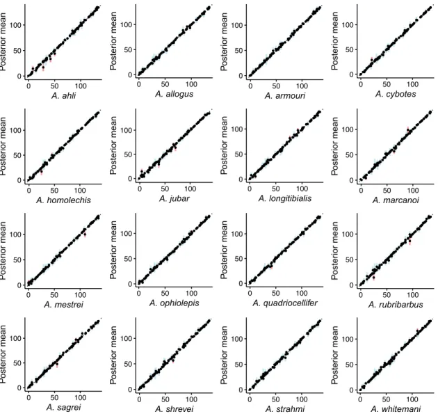
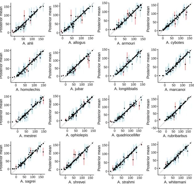
Figure S2: Species mean trait values simulated along the phylogeny under a WN process. Each panel shows the posterior mean of the mean trait value for the indicated species, as a function of the simulated trait mean. Vertical lines represent the 95% HPD intervals (blue if it includes the true value, red if it does not).
● ●● ● ● ● ● ● ● ● ● ● ● ● ● ●● ● ● ● ● ● ● ● ● ● ● ● ● ● ● ● ● ●● ● ● ● ●● ●● ● ● ● ● ● ● ● ●● ● ● ● ● ● ● ● ● ●● ● ● ● ● ● ● ● ●● ● ● ● ● ● ● ● ●● ● ● ● ● ●● ● ● ● ● ● ● ● ●● ● ●●● ● ● −20 0 20 40 60 −20 0 20 40 60 A. ahli Poste rior mean ● ● ● ● ● ● ● ● ● ● ● ● ● ● ● ● ● ● ● ● ● ● ● ● ● ● ● ●● ● ● ● ● ●● ● ● ● ● ● ● ● ● ● ● ● ● ● ●● ● ● ● ● ● ● ● ● ● ● ● ● ●● ● ● ● ● ● ● ● ● ● ●● ● ● ● ● ● ● ● ●● ● ● ● ● ● ● ● ● ● ● ● ● ● ● ●● −25 0 25 −25 0 25 A. allogus Poste rior mean ● ● ● ● ● ● ● ● ● ● ● ● ● ● ● ● ● ● ● ●● ● ● ● ● ● ● ● ● ● ● ● ● ● ● ● ● ● ● ● ● ● ● ● ● ● ● ● ● ● ● ● ● ● ● ● ● ● ● ● ● ● ● ● ● ● ● ●● ● ● ● ● ● ● ● ● ● ● ● ●● ●● ● ● ● ● ● ● ● ● ● ● ● ● ● ● ●● −20 0 20 40 −20 0 20 40 A. armouri Poste rior mean ●● ● ● ● ● ● ●● ●●● ● ● ● ● ● ● ● ● ● ● ● ● ● ● ● ● ● ● ● ● ● ● ● ● ● ● ● ● ● ● ● ● ● ● ●● ● ● ● ● ● ● ● ● ● ●● ● ● ● ● ● ● ● ● ● ● ● ● ● ● ● ●● ●● ● ● ● ● ● ● ● ● ● ● ● ● ● ● ● ● ● ● ● ● ● ● −40 −20 0 20 40 −40 −20 0 20 40 A. cybotes Poste rior mean ● ● ● ● ● ● ● ● ● ● ● ● ● ● ● ● ● ● ● ● ● ● ● ● ● ● ● ● ● ● ● ● ● ● ● ● ● ● ● ● ● ●● ● ● ● ● ● ●● ● ● ● ● ● ● ● ● ●● ● ● ● ● ●● ● ● ● ● ● ● ●● ●●● ●● ● ● ● ● ● ● ● ●● ● ● ● ● ● ● ●● ●● ● ● −30 0 30 −30 0 30 A. homolechis Poste rior mean ● ● ● ● ● ● ●● ● ● ● ● ● ● ● ● ● ● ● ● ● ● ● ● ● ● ● ● ● ● ● ● ● ● ● ● ● ●● ● ● ● ● ● ● ● ● ● ● ●● ● ● ● ● ● ● ●● ● ● ● ● ● ●●● ● ● ● ● ● ● ● ● ● ●●●●● ● ● ● ● ●● ● ● ●● ● ● ● ● ● ● ● ● ● −25 0 25 50 −25 0 25 50 A. jubar Poste rior mean ●● ● ● ● ● ● ● ● ● ● ● ● ● ● ● ●● ● ● ● ● ● ● ● ● ● ● ● ● ● ● ● ● ● ● ● ● ●● ● ● ● ● ● ●● ● ● ● ● ● ● ● ● ● ● ● ● ● ● ● ● ● ● ● ● ● ●● ● ●● ● ● ● ● ● ●● ● ● ● ● ● ● ● ● ● ● ●● ● ● ● ● ● ● ● ● −25 0 25 50 −25 0 25 50 A. longitibialis Poste rior mean ●● ● ● ● ● ● ● ● ● ● ● ● ● ● ● ●● ● ● ● ●● ● ● ● ●● ● ● ● ● ● ● ● ● ● ● ● ● ● ● ● ● ● ● ● ● ●● ● ● ● ● ●● ● ● ● ● ● ● ● ● ● ● ●● ● ● ● ● ● ● ● ● ● ● ● ● ● ● ● ●● ● ● ● ● ● ● ●● ● ● ● ● ●●● −50 −25 0 25 50 −50 −25 0 25 50 A. marcanoi Poste rior mean ● ● ● ● ● ● ●●● ● ● ● ● ● ● ● ●● ● ● ● ●● ● ● ● ● ● ● ● ● ● ● ● ● ● ●● ● ● ● ● ● ● ●● ● ● ● ● ● ● ●● ● ● ● ● ● ● ● ● ● ● ● ● ● ● ● ● ● ● ● ● ● ● ● ● ● ● ● ● ●● ● ● ● ●● ● ● ● ● ● ● ● ● ● ● ● −40 −20 0 20 −40 −20 0 20 A. mestrei Poste rior mean ● ● ● ● ● ● ●●●● ● ● ● ● ● ● ● ● ● ● ● ● ● ● ● ● ● ● ● ● ● ● ● ● ● ● ●● ● ● ● ● ● ● ● ● ● ● ● ● ●● ● ●● ● ● ● ● ● ● ● ● ● ● ● ● ● ● ● ● ● ● ● ● ●● ●● ● ●● ● ● ●● ● ● ● ● ● ● ● ● ● ● ● ● ● ● −20 0 20 40 −20 0 20 40 A. ophiolepis Poste rior mean ● ● ● ● ● ● ● ● ● ● ● ● ● ● ● ● ●● ● ● ● ● ● ● ● ● ● ● ● ● ● ● ● ● ● ● ● ● ● ● ● ● ● ● ● ● ● ● ● ● ●● ● ● ● ● ● ● ● ● ● ● ●● ●● ● ● ● ● ● ● ● ● ● ● ● ● ● ● ● ● ● ● ● ● ● ● ● ● ● ● ● ● ● ●●● ●● −20 0 20 40 60 −20 0 20 40 60 A. quadriocellifer Poste rior mean ● ● ● ● ● ● ● ● ● ● ● ● ● ● ● ● ● ● ● ● ● ● ● ● ● ● ● ● ● ● ● ● ● ● ● ● ● ● ● ● ● ● ● ● ● ● ● ● ●● ● ● ● ● ● ● ● ● ● ● ● ● ● ●● ● ● ● ● ● ● ● ● ● ● ● ●● ● ● ● ● ● ● ● ● ● ● ● ● ● ● ● ● ● ● ● ● ● ● −20 0 20 40 60 −20 0 20 40 60 A. rubribarbus Poste rior mean ● ●● ● ● ● ●●● ● ● ● ● ● ● ● ●● ● ● ● ●● ● ● ● ● ● ● ● ● ● ● ● ● ● ● ● ● ● ● ● ● ● ● ●● ● ● ●●● ● ● ● ●● ● ● ● ● ● ● ● ● ● ● ● ● ●● ● ● ●● ● ● ● ● ● ● ● ●● ● ● ● ● ● ●● ● ● ● ● ● ● ● ● ● −50 −25 0 25 50 −50 −25 0 25 50 A. sagrei Poste rior mean ● ● ● ● ● ● ● ●● ● ● ● ● ● ● ● ● ● ● ●● ● ● ● ● ● ● ● ● ● ● ● ● ● ● ● ● ● ● ● ● ● ● ● ● ● ● ● ● ● ● ● ● ● ● ● ● ● ● ● ● ● ● ● ● ● ● ● ● ● ● ● ●● ● ● ● ● ● ● ● ● ● ● ● ● ● ● ● ● ● ● ● ● ● ● ● ●● ● −20 0 20 40 −20 0 20 40 A. shrevei Poste rior mean ● ● ● ● ● ● ● ● ● ●● ● ● ● ● ● ● ● ● ● ● ● ● ●● ● ●● ● ● ● ● ● ● ● ● ● ●● ● ● ● ● ● ● ● ● ● ● ● ● ● ● ● ● ● ● ● ● ● ● ● ● ● ● ● ● ● ●● ● ● ● ● ● ● ● ● ● ● ● ● ●● ●● ● ● ● ● ● ● ● ● ● ● ● ● ● ● −25 0 25 50 −25 0 25 50 A. strahmi Poste rior mean ● ● ● ● ● ● ●● ● ● ● ● ● ● ● ● ● ● ● ● ●● ● ● ● ● ● ● ● ● ● ● ● ● ● ● ● ●● ● ● ● ● ● ● ● ● ●● ● ● ● ● ● ● ● ● ● ● ● ● ● ● ● ● ● ●● ●● ●● ● ● ● ● ● ●●● ● ● ● ● ● ● ● ● ● ● ● ● ● ● ● ● ● ● ● ● −20 0 20 40 −20 0 20 40 A. whitemani Poste rior mean
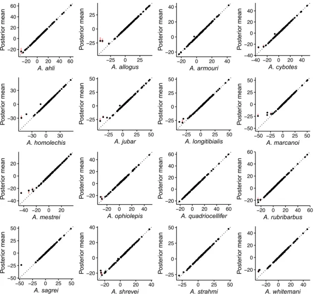
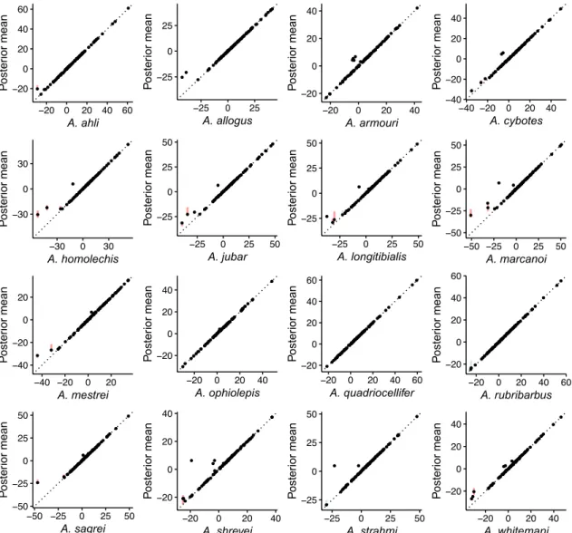
Figure S3: Species trait value log-variances simulated along the phylogeny under a BM process. Each panel shows the posterior mean of the trait value log-variance for the indicated species, as a function of the simulated trait mean. Vertical lines represent the 95% HPD intervals (blue if it includes the true value, red if it does not).
● ● ● ● ● ● ● ● ● ● ● ● ● ● ● ● ● ● ● ● ● ● ● ● ● ● ● ● ● ● ●● ● ● ● ● ● ● ● ● ● ● ● ● ● ● ● ● ● ● ●●● ● ●● ● ● ● ● ● ● ● ● ● ● ● ● ● ● ● ● ● ● ● ● ● ● ● ● ● ● ● ● ● ● ● ● ● ● ● ●● ● ● ● ● ● ● ● 0 10 20 0 10 20 σ12 Poste rior mean ● ● ● ● ● ● ● ● ● ● ● ● ●● ● ● ● ● ● ● ● ● ● ● ● ● ● ● ● ● ● ●● ● ● ● ● ● ● ● ● ● ● ● ● ● ● ● ● ● ● ● ● ● ● ● ● ● ● ●● ● ● ● ● ● ● ● ● ● ●●● ● ●● ● ●● ● ●● ● ● ● ● ● ● ● ● ● ● ● ● ● ● ● ● ● ● 0 10 20 30 0 10 20 30 σ22 Poste rior mean ● ● ● ● ● ● ● ● ● ● ● ● ● ● ● ● ● ● ● ● ● ● ● ● ● ● ● ● ● ● ● ● ● ● ● ● ● ● ● ● ● ● ● ● ● ● ● ● ●● ● ● ● ● ● ● ● ● ● ● ● ● ● ● ● ● ● ● ● ● ● ● ● ● ● ● ● ● ● ● ● ● ● ● ● ● ● ● ● ● ● ● ● ● ● ● ● ● ● ● 0 50 100 0 50 100 y0 Poste rior mean ● ● ● ● ● ● ● ● ● ● ● ● ● ● ● ● ● ● ● ● ● ● ● ●● ● ● ● ● ● ● ● ● ● ●● ● ● ● ● ● ● ● ● ● ● ● ● ●● ● ● ● ● ●● ● ● ● ● ● ● ●● ● ● ● ● ● ● ● ● ● ● ● ● ● ● ● ● ● ● ● ● ● ● ● ● ● ● ● ● ● ● ● ● ● ●● ● 0 5 10 15 20 0 5 10 15 20 σ2 Poste rior mean ● ● ● ● ● ● ● ● ● ● ● ● ● ● ● ● ● ● ● ● ● ● ● ● ● ● ● ● ● ●● ● ● ● ● ● ● ● ● ● ● ● ● ● ● ● ● ● ● ● ● ● ● ● ● ● ● ● ● ● ● ● ● ● ● ● ● ● ● ● ● ● ● ● ● ● ● ● ● ● ● ● ● ● ● ● ● ● ● ● ● ● ● ● ● ● ● ● ● ● 0 2 4 6 8 0 2 4 6 8 y0 Poste rior mean (b) (a)
Figure S4: Posterior means of prior parameters as a function of their simulated values. (a) Brow-nian motion prior with multiple evolutionary regimes (BMM) on species means. (b) BM prior on species log-variances. Vertical lines represent the 95% HPD intervals (blue if it includes the true value, red if it does not).
● ● ● ● ● ● ● ● ● ● ● ● ● ● ● ● ● ● ● ● ● ● ● ● ● ● ● ● ● ● ●● ● ● ● ● ● ● ● ● ● ● ● ● ● ● ● ● ●● ● ● ● ● ● ● ● ● ● ● ● ● ● ● ● ● ● ● ● ● ● ● ● ●● ● ● ● ● ● ● ● ● ● ● ● ● ● ● ● ● ● ● ● ● ● ● ● ● ● 0 50 100 150 0 50 100 150 A. ahli P oster ior mean ● ● ● ●● ● ● ● ● ● ● ● ● ● ● ● ● ● ● ● ● ● ● ● ● ● ● ● ● ● ● ● ● ● ● ● ● ● ● ● ● ● ● ● ● ● ● ● ●● ● ● ● ●● ● ● ● ● ● ● ●● ● ● ● ● ● ● ● ● ● ● ●● ● ● ● ● ● ● ● ● ● ● ● ● ● ● ● ● ● ● ● ● ● ● ● ● ● 0 50 100 150 0 50 100 150 A. allogus P oster ior mean ● ● ● ●● ● ● ● ● ● ● ● ● ● ● ● ● ● ● ● ● ● ●● ● ● ● ● ● ● ● ● ● ● ● ● ● ● ● ● ● ● ● ● ● ● ● ● ● ● ● ● ● ● ● ● ● ● ● ● ● ● ● ● ● ● ● ● ● ● ● ● ● ● ● ● ● ● ● ● ●● ● ● ● ● ● ● ● ● ● ● ●● ● ● ● ● ● ● 0 50 100 150 0 50 100 150 A. armouri P oster ior mean ● ● ● ● ● ● ● ● ● ●● ● ● ● ● ● ● ● ● ● ● ● ● ● ● ● ● ● ● ● ● ● ● ●● ● ● ● ● ● ● ● ● ● ● ● ● ● ● ● ● ● ● ● ● ● ● ● ● ● ● ● ● ● ● ● ● ● ● ● ● ● ● ● ● ● ● ● ● ● ● ●● ● ● ● ● ● ● ● ● ● ● ● ● ● ● ● ● ● 0 50 100 150 0 50 100 150 A. cybotes P oster ior mean ● ● ● ● ● ● ● ● ● ●● ● ● ● ● ● ● ● ● ● ● ●● ● ● ● ● ● ● ● ● ● ● ● ●● ● ● ● ● ● ● ● ● ● ● ● ● ● ● ● ● ● ● ● ●● ● ● ● ● ● ● ● ● ● ● ● ● ● ● ● ● ● ● ● ● ● ● ● ● ● ● ● ●● ● ● ● ● ● ● ● ● ● ●● ● ● ● 0 50 100 150 0 50 100 150 A. homolechis P oster ior mean ● ● ● ● ● ● ● ● ● ● ● ● ● ● ● ● ● ● ● ● ● ● ● ● ● ● ● ● ● ● ● ● ● ● ● ● ● ● ● ● ● ● ● ● ● ● ● ● ● ● ● ● ● ● ● ● ● ● ● ● ● ● ● ● ● ● ● ● ● ● ● ● ● ● ●● ● ● ● ● ● ● ● ● ● ● ● ● ● ● ● ● ● ● ● ●● ● ● ● 0 50 100 150 0 50 100 150 A. jubar P oster ior mean ● ● ● ● ● ● ● ● ● ●● ● ● ● ● ● ● ● ● ● ● ● ● ● ● ● ● ● ● ● ● ● ● ●● ● ● ● ● ● ● ● ● ● ● ● ● ● ● ● ● ● ● ● ●● ● ● ● ● ● ● ● ● ● ● ● ● ● ● ● ● ● ● ● ● ● ● ● ● ● ● ● ● ● ● ● ● ● ● ● ● ●● ● ● ● ● ● ● 0 50 100 150 0 50 100 150 A. longitibialis P oster ior mean ● ● ●● ● ● ● ● ● ● ● ● ● ● ● ● ● ● ● ● ● ● ● ● ● ● ● ● ● ● ● ● ● ● ● ● ●● ● ● ● ● ● ● ● ● ● ● ● ● ● ● ● ● ● ● ● ● ● ● ● ● ● ● ● ● ● ● ● ● ● ● ● ● ● ● ● ● ● ● ●● ● ● ● ● ● ● ● ●● ● ● ● ● ● ● ● ● ● 0 50 100 150 0 50 100 150 A. marcanoi P oster ior mean ● ● ● ● ● ● ● ● ● ● ● ● ● ● ● ● ● ● ● ● ● ● ●● ● ● ● ● ● ● ● ● ● ● ●● ● ● ● ● ● ● ● ● ● ● ● ●● ● ● ● ● ● ● ● ●● ● ● ● ● ● ● ● ● ● ● ● ●● ● ● ● ● ● ● ● ● ● ● ● ● ● ● ● ● ●● ● ● ● ● ● ● ●● ● ● ● 0 50 100 150 0 50 100 150 A. mestrei P oster ior mean ● ● ● ● ● ● ● ● ● ● ● ● ● ● ● ● ● ● ● ● ● ● ●● ● ● ● ● ● ● ● ● ● ● ● ● ● ● ● ● ● ● ● ● ● ● ● ● ● ● ● ● ● ● ● ●● ● ● ● ● ● ● ● ● ● ● ● ● ● ● ● ● ●● ● ● ● ● ● ● ● ● ● ● ● ● ● ● ● ● ● ● ● ● ● ● ● ● ● 0 50 100 150 0 50 100 150 A. ophiolepis P oster ior mean ● ● ● ● ● ● ● ● ● ● ● ● ● ● ● ● ● ● ● ● ● ● ● ● ● ● ● ● ● ● ● ● ● ● ● ● ● ● ● ● ● ● ● ● ● ● ● ● ●● ● ● ● ● ● ●●● ● ● ● ● ● ● ● ● ● ● ● ● ● ● ● ●● ● ● ● ● ● ● ● ●● ● ● ●● ● ●● ● ● ● ● ● ● ● ● ● 0 50 100 150 0 50 100 150 A. quadriocellifer P oster ior mean ● ● ● ● ● ● ● ● ● ●● ● ● ● ● ● ● ● ●● ● ● ● ● ● ● ● ● ● ● ● ● ● ● ● ● ● ● ● ● ● ● ● ● ● ● ● ● ●● ● ● ● ● ● ● ● ● ● ● ● ● ● ● ● ● ● ● ● ● ● ● ● ● ● ● ● ● ● ● ● ● ● ● ● ● ● ● ● ● ● ● ● ● ● ● ● ● ● ● −50 0 50 100 150 −50 0 50 100 150 A. rubribarbus P oster ior mean ● ● ● ● ● ● ● ● ● ● ● ● ● ● ● ● ● ● ● ● ● ● ●● ● ● ● ● ● ● ● ● ● ● ● ● ● ● ● ● ● ● ● ● ● ● ● ● ● ● ● ● ● ● ● ● ● ● ● ● ● ● ● ● ● ● ● ● ● ● ● ● ● ● ● ● ● ● ● ● ● ● ● ● ●● ● ● ● ● ● ● ● ● ● ● ● ● ● ● 0 50 100 150 0 50 100 150 A. sagrei P oster ior mean ● ● ●● ● ● ● ● ● ●● ● ● ● ● ● ● ● ● ● ● ● ● ●● ● ● ● ●● ● ● ● ● ● ● ●● ● ● ● ● ●● ●● ● ● ● ● ● ● ● ● ● ● ● ● ● ● ● ● ● ● ● ● ● ● ● ● ● ● ● ● ● ● ● ● ● ● ● ●● ● ● ● ● ● ● ● ● ● ● ● ● ●● ● ● ● 0 50 100 150 0 50 100 150 A. shrevei P oster ior mean ● ● ● ● ● ● ● ● ● ● ● ● ● ● ● ● ● ● ● ● ● ● ● ● ● ● ● ● ●● ● ● ● ● ● ● ● ● ● ● ● ● ●● ● ● ● ● ● ● ● ● ● ● ● ● ● ● ● ● ● ● ● ● ● ● ● ● ● ● ● ● ● ●● ● ● ●● ● ● ● ● ● ● ● ● ● ● ● ● ● ●● ● ● ● ● ● ● 0 50 100 150 0 50 100 150 A. strahmi P oster ior mean ● ● ●●● ● ● ● ● ● ● ● ● ● ● ● ● ● ● ● ● ● ● ● ● ● ● ● ●● ● ● ● ● ● ● ● ● ● ● ● ● ● ● ● ● ● ● ● ● ● ● ● ● ● ● ● ● ● ● ● ● ● ● ● ● ● ● ● ● ● ● ● ● ● ● ● ● ● ● ● ● ● ● ● ● ● ● ● ● ● ● ●● ● ● ● ●● ● 0 50 100 150 0 50 100 150 A. whitemani P oster ior mean
Figure S5: Species mean trait values simulated along the phylogeny under a Brownian motion process with multiple evolutionary regimes (BMM). Each panel shows the posterior mean of the mean trait value for the indicated species, as a function of the simulated trait mean. Vertical lines represent the 95% HPD intervals (blue if it includes the true value, red if it does not).
● ●● ● ● ● ● ● ● ● ● ● ● ● ● ●● ● ● ● ● ● ● ● ● ● ● ● ● ● ● ● ● ●● ● ● ● ●● ●● ● ● ● ● ● ● ● ●● ● ● ● ● ● ● ● ● ●● ● ● ● ● ● ● ● ●● ● ● ● ● ● ● ● ●● ● ● ● ● ●● ● ● ● ● ● ● ● ●● ● ●●● ● ● −20 0 20 40 60 −20 0 20 40 60 A. ahli Poste rior mean ● ● ● ● ● ● ● ● ● ● ● ● ● ● ● ● ● ● ● ● ● ● ● ● ● ● ● ●● ● ● ● ● ●● ● ● ● ● ● ● ● ● ● ● ● ● ● ●● ● ● ● ● ● ● ● ● ● ● ● ● ●● ● ● ● ● ● ● ● ● ● ●● ● ● ● ● ● ● ● ●● ● ● ● ● ● ● ● ● ● ● ● ● ● ● ●● −25 0 25 −25 0 25 A. allogus Poste rior mean ● ● ● ● ● ● ● ● ● ● ● ● ● ● ● ● ● ● ● ●● ● ● ● ● ● ● ● ● ● ● ● ● ● ● ● ● ● ● ● ● ● ● ● ● ● ● ● ● ● ● ● ● ● ● ● ● ● ● ● ● ● ● ● ● ● ● ●● ● ● ● ● ● ● ● ● ● ● ● ●● ●● ● ● ● ● ● ● ● ● ● ● ● ● ● ● ●● −20 0 20 40 −20 0 20 40 A. armouri Poste rior mean ●● ● ● ●●● ●● ●●● ● ● ● ● ● ● ● ● ● ● ● ● ● ● ● ● ● ● ● ● ● ● ● ● ● ● ● ● ● ● ● ● ● ● ●● ● ● ● ● ● ● ● ● ● ●● ● ● ● ● ● ● ● ● ● ● ● ● ● ● ● ●● ●● ● ● ● ● ● ● ● ● ● ● ● ● ● ● ● ● ● ● ● ● ● ● −40 −20 0 20 40 −40 −20 0 20 40 A. cybotes Poste rior mean ● ● ● ● ● ● ● ● ● ● ● ● ● ● ● ● ● ● ● ● ● ● ● ● ● ● ● ● ● ● ● ● ● ● ● ● ● ● ● ● ● ●● ● ● ● ● ● ●● ● ● ● ● ● ● ● ● ●● ● ● ● ● ●● ● ● ● ● ● ● ●● ●●● ●● ● ● ● ● ● ● ● ●● ● ● ● ● ● ● ●● ●● ● ● −30 0 30 −30 0 30 A. homolechis Poste rior mean ● ● ● ● ● ● ●● ● ● ● ● ● ● ● ● ● ● ● ● ● ● ● ● ● ● ● ● ● ● ● ● ● ● ● ● ● ●● ● ● ● ● ● ● ● ● ● ● ●● ● ● ● ● ● ● ●● ● ● ● ● ● ●●● ● ● ● ● ● ● ● ● ● ●●● ● ● ● ● ● ● ●● ● ● ●● ● ● ● ● ● ● ● ● ● −25 0 25 50 −25 0 25 50 A. jubar Poste rior mean ●● ● ● ● ● ● ● ● ● ● ● ● ● ● ● ●● ● ● ● ● ● ● ● ● ● ● ● ● ● ● ● ● ● ● ● ● ●● ● ● ● ● ● ●● ● ● ● ● ● ● ● ● ● ● ● ● ● ● ● ● ● ● ● ● ● ●● ● ● ● ● ● ● ● ● ●● ● ● ● ● ● ● ● ● ● ● ●● ● ● ● ● ● ● ● ● −25 0 25 50 −25 0 25 50 A. longitibialis Poste rior mean ●● ● ● ● ● ● ● ● ● ● ● ● ● ● ● ●● ● ● ● ●● ● ● ● ●● ● ● ● ● ● ● ● ● ● ● ● ● ● ● ● ● ● ● ● ● ● ● ● ● ● ● ● ● ● ● ● ● ● ● ● ● ● ● ●● ● ● ● ● ● ● ● ● ● ● ● ● ● ● ● ●● ● ● ● ● ● ● ●● ● ● ● ● ●●● −50 −25 0 25 50 −50 −25 0 25 50 A. marcanoi Poste rior mean ● ● ● ● ● ● ●●● ● ● ● ● ● ● ● ●● ● ● ● ●● ● ● ● ● ● ● ● ● ● ● ● ● ● ●● ● ● ● ● ● ● ● ● ● ● ● ● ● ● ●● ● ● ● ● ● ● ● ● ● ● ● ● ● ● ● ● ● ● ● ● ● ● ● ● ● ● ● ● ●● ● ● ● ● ● ● ● ● ● ● ● ● ● ● ● ● −40 −20 0 20 −40 −20 0 20 A. mestrei Poste rior mean ● ● ● ● ● ● ●●●● ● ● ● ● ● ● ● ● ● ● ● ● ● ● ● ● ● ● ● ● ● ● ● ● ● ● ●● ● ● ● ● ● ● ● ● ● ● ● ● ●● ● ●● ● ● ● ● ● ● ● ● ● ● ● ● ● ● ● ● ● ● ● ● ●● ●● ● ●● ● ● ●● ● ● ● ● ● ● ● ● ● ● ● ● ● ● −20 0 20 40 −20 0 20 40 A. ophiolepis Poste rior mean ● ● ● ● ● ● ● ● ● ● ● ● ● ● ● ● ●● ● ● ● ● ● ● ● ● ● ● ● ● ● ● ● ● ● ● ● ● ● ● ● ● ● ● ● ● ● ● ● ● ● ● ● ● ● ● ● ● ● ● ● ● ●● ●● ● ● ● ● ● ● ● ● ● ● ● ● ● ● ● ● ● ● ● ● ● ● ● ● ● ● ● ● ● ●●● ●● −20 0 20 40 60 −20 0 20 40 60 A. quadriocellifer Poste rior mean ● ● ● ● ● ● ● ● ● ● ● ● ● ● ● ● ● ● ● ● ● ● ● ● ● ● ● ● ● ● ● ● ● ● ● ● ● ● ● ● ● ● ● ● ● ● ● ● ●● ● ● ● ● ● ● ● ● ● ● ● ● ● ●● ● ● ● ● ● ● ● ● ● ● ● ●● ● ● ● ● ● ● ● ● ● ● ● ● ● ● ●● ● ● ● ● ● ● −20 0 20 40 60 −20 0 20 40 60 A. rubribarbus Poste rior mean ● ●● ● ● ● ●●● ● ● ● ● ● ● ● ●● ● ● ● ●● ● ● ● ● ● ● ● ● ● ● ● ● ● ● ● ● ● ● ● ● ● ● ●● ● ● ●●●● ● ● ●● ● ● ● ● ● ● ● ● ● ● ● ● ●● ● ● ●● ● ● ● ● ● ● ● ●● ● ● ● ● ● ●● ● ● ● ● ● ● ● ● ● −50 −25 0 25 50 −50 −25 0 25 50 A. sagrei Poste rior mean ● ● ● ● ● ● ● ●● ● ● ● ● ● ● ● ● ● ● ●● ● ● ● ● ● ● ● ● ● ● ● ● ● ● ● ● ● ● ● ● ● ● ● ● ● ● ● ●● ● ● ● ● ● ● ● ● ● ● ● ● ● ● ● ● ● ● ● ● ● ● ●● ● ● ● ● ● ● ● ● ● ● ● ● ● ● ● ● ● ● ● ● ● ● ● ● ● ● −20 0 20 40 −20 0 20 40 A. shrevei Poste rior mean ● ● ● ● ● ● ● ● ● ●● ● ● ● ● ● ● ● ● ● ● ● ● ●● ● ●● ● ● ● ● ● ● ● ● ● ●● ● ● ● ● ● ● ● ● ● ● ● ● ● ● ● ● ● ● ● ● ● ● ● ● ● ● ● ● ● ●● ● ● ● ● ● ● ● ● ● ● ● ● ●● ●● ● ● ● ● ● ● ● ● ● ● ● ● ● ● −25 0 25 50 −25 0 25 50 A. strahmi Poste rior mean ●● ● ● ● ● ●● ● ● ● ● ● ● ● ● ● ● ● ● ●● ● ● ● ● ● ● ● ● ● ● ● ● ● ● ● ●● ● ● ● ● ● ● ● ● ● ● ● ● ● ● ● ● ● ● ● ● ● ● ● ● ● ● ● ●● ●● ● ● ● ● ● ● ● ●●● ● ● ● ● ● ● ● ● ● ● ● ● ● ● ● ● ● ● ● ● −20 0 20 40 −20 0 20 40 A. whitemani Poste rior mean
Figure S6: Species trait values log-variances simulated along the phylogeny under a Brownian motion process with multiple evolutionary regimes (BMM). Each panel shows the posterior mean of the trait value variance for the indicated species, as a function of the simulated trait log-variance. Vertical lines represent the 95% HPD intervals (blue if it includes the true value, red if it does not).
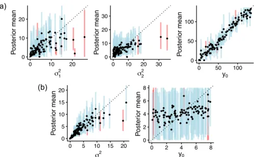
(b) (a) ● ●● ● ● ● ● ● ● ●●● ● ● ● ● ● ● ● ● ● ● ● ● ● ● ● ● ● ● ● ●●● ● ● ● ● ● ● ● ●●● ● ● ● ● ● ● ● ● ● ● ● ● ●● ● ● ● ● ● ● ● ● ● ● ● ● ● ● ● ● ● ● ● ● ● ● ● ● ● ● ● ● ● ● ● ● ●●● ● ● ●● ● ● ● 0 10 20 30 40 50 0 10 20 30 40 50 σ2 Poste rior mean ● ● ● ● ● ● ● ● ● ● ● ● ● ● ● ● ● ● ● ● ● ● ● ● ● ● ● ● ● ● ● ● ● ● ● ● ● ● ● ● ● ● ● ● ● ● ● ● ● ● ● ● ●● ● ● ● ● ● ●● ● ● ● ● ● ● ● ● ● ● ● ●● ● ● ● ● ● ● ●● ● ● ● ● ● ● ● ● ● ● ● ● ● ● ● ● ● ● 0 10 20 30 0 10 20 30 α Poste rior mean ● ●● ●● ● ● ● ● ● ● ● ● ● ● ● ● ● ● ●● ● ● ● ● ● ● ● ● ● ● ● ● ● ● ● ● ● ● ● ● ● ● ● ● ● ● ● ● ● ● ● ● ● ● ●● ● ● ● ● ● ● ● ● ● ● ● ● ● ● ● ● ● ● ● ● ● ● ● ● ● ● ● ● ● ● ● ● ● ● ● ● ● ● ● ● ● ● ● 0 50 100 0 50 100 θ1 Poste rior mean ● ● ● ● ● ● ● ● ● ● ● ● ● ● ● ● ● ● ● ● ● ● ● ● ●● ● ● ● ● ● ● ● ● ● ● ● ● ● ● ● ● ● ● ● ● ● ● ● ● ● ● ● ● ● ● ● ● ● ● ● ● ● ● ● ● ● ● ● ● ● ● ● ● ● ● ● ● ● ● ● ● ● ● ● ● ● ● ● ● ● ● ●● ● ● ● ● ● ● 0 50 100 0 50 100 θ2 Poste rior mean ● ● ● ● ● ● ● ● ● ● ● ● ● ● ● ● ● ● ● ● ●● ● ● ● ● ● ● ●● ● ● ●● ● ● ● ● ● ● ● ● ● ● ● ● ● ● ● ● ● ● ● ● ●● ● ● ● ● ● ● ● ● ● ● ● ● ● ● ● ● ● ● ● ● ● ● ● ● ● ● ● ● ● ● ● ● ● ● ● ● ● ● ● ● ● ● ● ● 0 5 10 15 20 0 5 10 15 20 σ2 Poste rior mean ● ● ● ● ● ● ● ● ● ● ● ● ● ● ● ● ● ● ● ● ● ● ● ● ● ● ● ● ● ● ● ● ● ● ● ● ● ● ● ● ● ● ● ● ● ● ● ● ● ● ● ● ● ● ● ● ● ● ● ● ● ● ● ● ● ● ● ● ● ● ● ● ● ● ● ● ● ● ● ● ● ● ● ● ● ● ● ● ● ● ● ● ● ● ● ● ● ● ● ● 0 2 4 6 8 0 2 4 6 8 y0 Poste rior mean
Figure S7: Posterior means of prior parameters as a function of their simulated values. (a) Ornstein-Uhlenbeck prior with multiple evolutionary regimes (OUM) on species means. (b) BM prior on species log-variances. Vertical lines represent the 95% HPD intervals (blue if it includes the true value, red if it does not).
● ●● ● ● ● ● ● ● ● ● ● ● ● ● ● ● ● ● ● ● ● ● ● ● ● ● ● ● ● ● ● ● ● ● ● ● ● ● ● ● ● ● ● ● ● ● ● ● ● ● ● ● ● ● ●● ● ● ● ● ● ● ● ● ● ● ● ● ● ● ● ● ● ● ● ● ● ● ● ● ● ● ● ● ● ● ● ● ● ● ● ● ● ● ● ● ● ● ● 0 50 100 0 50 100 A. ahli Poste rior mean ● ● ● ● ● ● ● ● ● ● ● ● ● ● ● ● ● ● ● ● ● ● ● ● ● ● ● ● ● ● ● ● ● ● ● ● ● ● ● ● ● ● ● ● ● ● ● ● ● ● ● ● ● ● ● ●● ● ● ● ● ● ● ● ● ● ● ● ● ● ● ● ● ● ● ● ● ● ● ● ● ● ● ● ● ● ● ● ● ● ● ● ● ● ● ● ● ● ● ● 0 50 100 0 50 100 A. allogus Poste rior mean ● ● ● ● ● ● ● ● ● ● ● ● ● ● ● ● ● ● ● ● ● ● ● ● ●● ● ● ● ● ● ● ● ● ● ● ● ● ● ● ● ● ● ● ● ● ● ● ● ● ● ● ● ● ● ● ● ● ● ● ● ● ● ● ● ● ● ● ● ● ● ● ● ● ● ● ● ● ● ● ● ● ● ● ● ● ● ● ● ● ● ● ●● ● ● ● ● ● ● 0 50 100 0 50 100 A. armouri Poste rior mean ● ● ● ● ● ● ● ● ● ● ● ● ● ● ●● ● ● ● ● ● ● ● ● ●● ● ● ● ● ● ● ● ● ● ● ● ● ● ● ● ● ● ● ● ● ● ● ● ● ● ● ● ● ● ● ● ● ● ● ● ● ● ● ● ● ● ● ● ● ● ● ● ● ● ● ● ● ● ● ● ● ● ● ● ● ● ● ● ● ● ● ●● ● ● ● ● ● ● 0 50 100 0 50 100 A. cybotes Poste rior mean ● ●● ●● ● ● ● ● ● ● ● ● ● ● ● ● ● ● ●● ● ● ● ● ● ● ● ● ● ● ● ● ● ● ● ● ● ● ● ● ● ● ● ● ● ● ● ● ● ● ● ● ● ● ● ● ● ● ● ● ● ● ● ● ● ● ● ● ● ● ● ● ● ● ● ● ● ● ● ● ● ● ● ● ● ● ● ● ● ● ● ● ● ● ● ● ● ● ● 0 50 100 0 50 100 A. homolechis Poste rior mean ● ●● ●● ● ● ● ● ● ● ● ● ● ● ● ● ● ● ● ● ● ● ● ● ● ● ● ● ● ● ● ● ● ● ● ● ● ● ● ● ● ● ● ● ● ● ● ● ● ● ● ● ● ● ●● ● ● ● ● ● ● ● ● ● ● ● ● ● ● ● ●● ● ● ● ● ● ● ● ● ● ● ● ● ● ● ● ● ● ● ● ● ● ● ● ● ● ● 0 50 100 150 0 50 100 150 A. jubar Poste rior mean ● ● ● ● ● ● ● ● ● ● ● ● ● ● ●● ● ● ● ● ● ● ● ● ●● ● ● ● ● ● ● ● ● ● ● ● ● ● ● ● ● ● ● ● ● ● ●● ● ● ● ● ● ● ● ● ● ● ● ● ● ● ● ● ● ● ● ● ● ● ● ● ● ● ● ● ● ● ● ● ● ● ● ● ● ● ● ● ● ● ● ●● ● ● ● ● ● ● 0 50 100 0 50 100 A. longitibialis Poste rior mean ● ● ● ● ● ● ● ● ● ● ● ● ● ● ● ● ● ● ● ● ● ● ● ● ●● ● ● ● ● ● ● ● ● ● ● ● ● ● ● ● ● ● ● ● ● ● ● ● ● ● ● ● ● ● ● ● ● ● ● ● ● ● ● ● ● ● ● ● ● ● ● ● ● ● ● ● ● ● ● ● ● ● ● ● ● ● ● ● ● ● ● ●● ● ● ● ● ● ● 0 50 100 0 50 100 A. marcanoi Poste rior mean ● ●● ● ● ● ● ● ● ● ● ● ● ● ● ● ● ● ● ●● ● ● ● ● ● ● ● ● ● ● ● ● ● ● ● ● ● ● ● ● ● ● ● ● ● ● ● ● ● ● ● ● ● ● ●● ● ● ● ● ● ● ● ● ● ● ● ● ● ● ● ● ● ● ● ● ● ● ● ● ● ● ● ● ● ● ● ● ● ● ● ● ● ● ● ● ● ● ● 0 50 100 0 50 100 A. mestrei Poste rior mean ● ●● ●● ● ● ● ● ● ● ● ● ● ● ● ● ● ● ●● ● ● ● ● ● ● ● ● ● ● ● ● ● ● ● ● ● ● ● ● ● ● ● ● ● ● ● ● ● ● ● ● ● ● ●● ● ● ● ● ● ● ● ● ● ● ● ● ● ● ● ● ● ● ● ● ● ● ● ● ● ● ● ● ● ● ● ● ● ● ● ● ● ● ● ● ● ● ● 0 50 100 0 50 100 A. ophiolepis Poste rior mean ● ●● ●● ● ● ● ● ● ● ● ● ● ● ● ● ● ● ●● ● ● ● ● ● ● ● ● ● ● ● ● ● ● ● ● ● ● ● ● ● ● ● ● ● ● ● ● ● ● ● ● ● ● ●● ● ● ● ● ● ● ● ● ● ● ● ● ● ● ● ● ● ● ● ● ● ● ● ● ● ● ● ● ● ● ● ● ● ● ● ● ● ● ● ● ● ● ● 0 50 100 0 50 100 A. quadriocellifer Poste rior mean ● ●● ● ● ● ● ● ● ● ● ● ● ● ● ● ● ● ● ● ● ● ● ● ● ● ● ● ● ● ● ● ● ● ● ● ● ● ● ● ● ● ● ● ● ● ● ● ● ● ● ● ● ● ● ●● ● ● ● ● ● ● ● ● ● ● ● ● ● ● ● ● ● ● ● ● ● ● ● ● ● ● ● ● ● ● ● ● ● ● ● ● ● ● ● ● ● ● ● 0 50 100 0 50 100 A. rubribarbus Poste rior mean ● ●● ●● ● ● ● ● ● ● ● ● ● ● ● ● ● ● ● ● ● ● ● ● ● ● ● ● ● ● ● ● ● ● ● ● ● ● ● ● ● ● ● ● ● ● ● ● ● ● ● ● ● ● ●● ● ● ● ● ● ● ● ● ● ● ● ● ● ● ● ● ● ● ● ● ● ● ● ● ● ● ● ● ● ● ● ● ● ● ● ● ● ● ● ● ● ● ● 0 50 100 0 50 100 A. sagrei Poste rior mean ● ● ● ● ● ● ● ● ● ● ● ● ● ● ●● ● ● ● ● ● ● ● ● ●● ● ● ● ● ● ● ● ● ● ● ● ● ● ● ● ● ● ● ● ● ● ● ● ● ● ● ● ● ● ● ● ● ● ● ● ● ● ● ● ● ● ● ● ● ● ● ● ● ● ● ● ● ● ● ● ● ● ● ● ● ● ● ● ● ● ● ●● ● ● ● ● ● ● 0 50 100 0 50 100 A. shrevei Poste rior mean ● ● ● ● ● ● ● ● ● ● ● ● ● ● ● ● ● ● ● ● ● ● ● ● ●● ● ● ● ● ● ● ● ● ● ● ● ● ● ● ● ● ● ● ● ● ● ● ● ● ● ● ● ● ● ● ● ● ● ● ● ● ● ● ● ● ● ● ● ● ● ● ● ● ● ● ● ● ● ● ● ● ● ● ● ● ● ● ● ● ● ● ●● ● ● ● ● ● ● 0 50 100 0 50 100 A. strahmi Poste rior mean ● ● ● ● ● ● ● ● ● ● ● ● ● ● ● ● ● ● ● ● ● ● ● ● ●● ● ● ● ● ● ● ● ● ● ● ● ● ● ● ● ● ● ● ● ● ● ● ● ● ● ● ● ● ● ● ● ● ● ● ● ● ● ● ● ● ● ● ● ● ● ● ● ● ● ● ● ● ● ● ● ● ● ● ● ● ● ● ● ● ● ● ●● ● ● ● ● ● ● 0 50 100 0 50 100 A. whitemani Poste rior mean
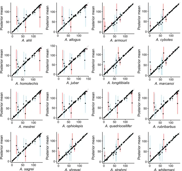
Figure S8: Species mean trait values simulated along the phylogeny under an Ornstein-Uhlenbeck process with multiple evolutionary regimes (OUM). Each panel shows the posterior mean of the mean trait value for the indicated species, as a function of the simulated trait mean. Vertical lines represent the 95% HPD intervals (blue if it includes the true value, red if it does not).
●● ● ● ● ●● ● ● ● ● ● ● ● ● ● ● ● ● ● ● ● ● ● ● ● ●●●● ● ● ●● ● ● ● ● ● ● ●● ● ● ● ● ● ● ● ● ● ● ● ● ●● ● ●● ●● ● ● ● ● ● ● ● ●● ● ● ● ● ● ● ● ● ● ● ● ● ● ●● ● ● ●● ● ● ● ● ● ● ● ●● ● ● −30 0 30 60 90 −30 0 30 60 90 A. ahli Poste rior mean ● ● ● ● ● ● ● ● ● ● ● ●● ● ● ● ●● ● ● ● ● ● ● ● ● ● ● ● ● ● ● ● ● ● ● ● ● ● ● ● ● ● ● ●● ● ● ● ● ● ● ● ● ● ● ● ● ● ● ● ● ● ● ● ● ● ● ● ● ● ● ● ● ● ● ● ●● ●● ● ● ● ● ● ● ● ●●●● ● ● ● ● ● ● ● ● −25 0 25 50 75 −25 0 25 50 75 A. allogus Poste rior mean ● ●● ● ● ● ● ● ● ● ● ● ● ● ● ● ● ● ● ● ● ● ● ● ● ● ● ● ● ● ● ● ● ● ● ● ● ● ● ● ● ● ● ● ● ● ● ● ● ● ● ●● ● ● ● ● ● ● ● ● ● ● ●● ● ● ●●● ● ● ● ● ● ● ● ● ● ● ●● ● ●● ● ● ● ● ● ● ● ● ● ● ● ● ● ●● −20 0 20 40 −20 0 20 40 A. armouri Poste rior mean ● ● ● ● ● ● ● ● ● ●● ● ● ● ● ● ● ● ● ●● ● ● ● ● ● ● ● ● ● ● ● ● ● ● ● ● ● ● ● ● ● ● ● ● ● ● ● ● ● ● ● ● ● ●● ● ● ● ● ● ● ● ●● ● ● ● ● ● ● ● ● ● ● ● ● ● ● ● ● ● ● ● ● ● ● ● ● ● ●● ● ● ● ● ● ● ● ● −40 −20 0 20 −40 −20 0 20 A. cybotes Poste rior mean ● ● ● ● ● ● ● ● ● ● ● ●●● ●● ● ● ● ● ● ● ● ● ● ● ● ● ●● ● ● ● ●● ● ● ● ● ● ● ● ● ● ● ● ● ● ●● ● ● ●● ● ● ● ● ● ● ● ● ● ● ● ●● ● ● ● ● ● ● ● ●●●● ● ● ● ● ● ● ● ● ● ● ● ● ● ● ● ● ● ● ● ● ● ● −60 −30 0 30 60 −60 −30 0 30 60 A. homolechis Poste rior mean ● ● ● ● ● ● ● ● ● ● ● ●●● ● ● ● ● ● ● ● ●● ● ● ● ● ● ●● ● ● ● ● ● ● ●●●● ● ● ● ● ● ● ● ● ● ● ● ● ● ● ● ● ● ●● ● ●● ● ● ● ● ● ● ● ● ● ● ● ● ●● ●● ● ● ● ● ● ● ● ●● ● ● ● ● ● ● ● ● ● ● ● ● ● −25 0 25 −25 0 25 A. jubar Poste rior mean ● ● ● ● ● ● ● ● ● ● ● ● ● ● ● ● ● ● ● ● ● ● ● ● ● ● ● ● ● ● ● ● ● ● ● ● ●● ● ● ● ● ● ● ●● ● ● ● ● ● ●● ● ● ● ● ● ● ● ● ● ● ● ●● ● ● ● ● ● ● ● ● ● ● ● ● ● ● ● ● ● ● ● ● ● ● ● ● ●● ● ● ● ● ● ● ● ● −40 −20 0 20 −40 −20 0 20 A. longitibialis Poste rior mean ● ● ● ● ● ● ● ● ● ● ● ● ● ●● ● ● ● ● ● ● ● ● ● ● ● ● ● ● ● ● ● ● ● ● ● ● ● ● ● ● ● ● ● ● ● ● ●● ● ● ● ● ●● ● ● ● ● ● ● ● ● ●● ● ● ● ● ● ● ● ● ● ● ● ●● ●● ● ● ● ●● ● ● ●● ● ● ● ● ● ● ● ● ● ● ● −50 −25 0 25 −50 −25 0 25 A. marcanoi Poste rior mean ● ● ● ● ● ● ● ● ● ● ● ● ● ● ●● ● ● ● ● ●● ● ● ● ● ● ● ● ● ● ● ● ● ● ● ●● ● ● ● ● ● ●●● ● ● ● ●● ● ● ● ● ● ● ● ● ● ●● ● ● ● ●● ● ● ●● ● ● ● ● ● ● ● ● ● ● ● ●● ● ● ● ● ● ● ● ● ● ● ● ●● ●●● −50 −25 0 25 50 −50 −25 0 25 50 A. mestrei Poste rior mean ● ● ● ● ● ● ● ● ● ● ● ● ●● ● ● ●● ● ● ● ● ● ● ● ● ● ● ● ● ● ● ● ● ● ● ● ● ● ● ● ● ● ● ● ● ● ● ● ● ● ● ● ● ● ● ● ● ● ● ● ●● ● ● ●● ● ● ● ● ● ● ● ● ● ● ● ● ● ● ● ● ● ● ● ● ● ● ● ●●● ● ● ●● ● ● ● −20 0 20 40 −20 0 20 40 A. ophiolepis Poste rior mean ● ● ● ● ● ● ●● ● ● ● ● ●● ● ●● ● ● ● ● ● ● ● ● ● ● ● ●●● ● ● ● ● ● ● ● ● ● ● ● ● ● ● ● ●● ● ● ● ● ● ● ● ● ● ● ● ● ● ● ● ● ● ●● ● ● ● ● ● ●● ● ● ● ● ● ● ● ● ● ● ● ● ● ● ● ● ● ● ● ● ● ● ● ● ● ● −20 0 20 40 60 −20 0 20 40 60 A. quadriocellifer Poste rior mean ●● ● ● ● ● ● ● ● ● ● ● ● ● ● ● ● ● ● ● ● ● ● ● ● ● ● ● ●● ●● ● ● ● ● ● ● ● ● ● ● ● ●● ●● ● ● ● ● ● ● ● ● ● ● ● ● ● ● ● ● ● ● ● ● ● ● ● ● ● ● ● ● ● ●● ● ● ● ● ● ● ● ● ● ● ● ● ●● ● ● ● ● ● ● ● ● −20 0 20 40 60 −20 0 20 40 60 A. rubribarbus Poste rior mean ● ● ● ● ● ● ● ● ● ● ● ● ● ●● ● ● ● ● ● ●● ● ● ● ● ● ● ● ● ● ● ● ● ● ● ● ● ● ● ● ● ● ● ● ● ● ● ● ● ● ● ● ● ● ● ● ● ● ● ● ● ● ● ● ● ● ● ●● ● ● ● ● ● ● ● ● ● ● ● ● ● ● ● ● ● ● ● ● ● ● ● ● ● ● ●● ● ● −20 0 20 −20 0 20 A. sagrei Poste rior mean ● ● ● ● ● ● ● ● ● ● ● ● ● ● ● ● ● ● ● ●● ● ●● ● ● ● ● ● ● ● ● ● ● ● ● ● ● ● ● ● ● ● ● ● ● ● ● ● ● ● ●●● ● ● ● ● ● ● ● ● ● ● ● ● ● ● ● ● ● ● ● ● ● ● ● ● ●● ● ● ● ● ● ● ● ● ● ● ●● ● ● ● ● ● ● ● ● −25 0 25 −25 0 25 A. shrevei Poste rior mean ● ● ● ● ●● ● ● ● ● ● ● ●● ● ● ● ● ● ● ● ● ● ● ● ● ● ● ● ● ● ● ● ●● ● ● ●● ● ● ● ● ● ● ● ● ● ● ● ● ● ● ● ● ● ● ● ● ● ● ● ● ● ●● ● ● ● ● ● ● ● ● ● ● ● ● ● ● ● ● ● ● ● ● ● ● ● ● ●● ● ● ● ● ● ● ● ● −20 0 20 −20 0 20 A. strahmi Poste rior mean ● ● ● ● ● ● ● ● ● ● ●● ● ● ● ● ● ● ● ●● ● ● ● ● ● ● ● ● ● ● ● ● ● ● ● ● ●● ● ● ● ●● ● ● ● ● ● ● ● ●● ● ●● ● ● ● ● ● ● ● ● ● ● ● ● ● ● ● ● ● ● ● ● ● ● ● ● ● ● ● ● ● ● ● ● ● ● ●●● ● ● ● ● ● ●● −25 0 25 −25 0 25 A. whitemani Poste rior mean
Figure S9: Species trait values log-variances simulated along the phylogeny under an Ornstein-Uhlenbeck process with multiple evolutionary regimes (OUM). Each panel shows the posterior mean of the trait value log-variance for the indicated species, as a function of the simulated trait log-variance. Vertical lines represent the 95% HPD intervals (blue if it includes the true value, red if it does not).
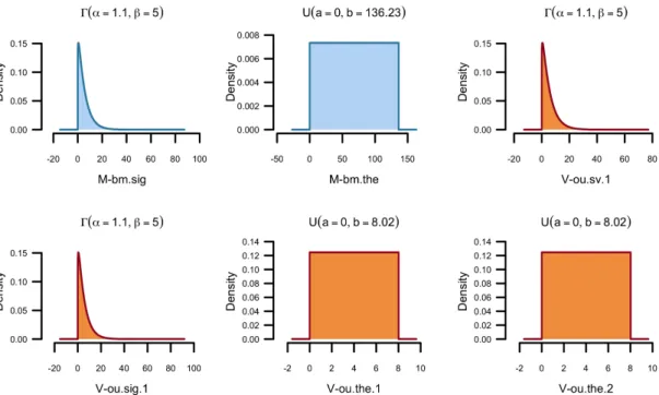
Figure S10: Example output of plot hp(). These plots represent the prior distribution of the parameters used in the evolutionary models for means (blue) and variances (orange). M-bm.the:
θ0m, trait mean value at the root, M-bm.sig: σm2, evolutionary rate of the trait mean, V-ou.the.1:
θvH, optimal trait variance for the “cybotes” clade, V-ou.the.2: θvC, optimal trait variance for the
“sagrei” clade, V-ou.sv.1: stationary variance of the trait variance, V-ou.sig.1: σ2
v, evolutionary rate of the trait variance
0 500000 1000000 1500000 2000000 2.5 3.0 3.5 4.0 Iterations var .ou.the .H ESS = 848.33 ; HPD [2.94,3.66] ; mean = 3.31 0.0 0.5 1.0 1.5 2.0 Density
Figure S11: Example output of the plot mcmc bite() function. The plots represent the traces and posterior distributions of prior parameters for the mean and log-variances under the mBM-vOUM model. The shaded area in the trace plot represents the burn-in phase. Above each trace the estimated effective sample size (ESS) and the highest posterior density (HPD) are indi-cated as well as the mean estimate. mean.bm.the: θ0m, trait mean value at the root, mean.bm.sig: σ2
m, evolutionary rate of the trait mean, var.ou.the.H: θvH, optimal trait variance for the “cybotes”
clade, var.ou.the.C: θvC, optimal trait variance for the “sagrei” clade, var.ou.sv: stationary variance
Figure S12: Maximum-credibility Anolis tree estimated from molecular and inter- and intraspe-cific continuous trait data (using BEAST 2). Nodes are colored according to their mean posterior probabilities of having incurred a θ-shift in trait log-variances (i.e., δ), under the vOUM model. Bars correspond to 95% highest posterior density intervals for divergence times, and numbers next to nodes to posterior clade probabilities.
Figure S13: Example output of plot pvo(). The phylogenetic tree is represented with the mapped regimes colored in green (Hispaniola) and blue (Cuba). Facing every tip of the tree is the posterior distribution of snout-to-vent-length sampled under the mBM-vOUM model. Those distribution were obtained from estimated means and variances using highest posterior densities of both variables. The “lollipops” represent observations used in the model.
References
[1] Alf¨oldi, J. et al. (2011). The genome of the green anole lizard and a comparative analysis with birds and mammals. Nature, 477:587–591.
[2] Bastide, P., An´e, C., Robin, S., and Mariadassou, M. (2018). Inference of adaptive shifts for multivariate correlated traits. Syst. Biol., 67:662–80.
[3] Clavel, J., Escarguel, G., and Merceron, G. (2015). mvMORPH: an R package for fitting mul-tivariate evolutionary models to morphometric data. Methods Ecol. Evol., 6:1311–1319.
[4] Drummond, A. J. and Suchard, M. A. (2010). Bayesian random local clocks, or one rate to rule them all. BMC Biol., 8.
[5] Heled, J. and Drummond, A. J. (2012). Calibrated tree priors for relaxed phylogenetics and divergence time estimation. Syst. Biol., 61:138–49.
[6] Ho, L. S. T. and An´e, C. (2013). Asymptotic theory with hierarchical autocorrelation: Ornstein–Uhlenbeck tree models. Ann. Stat., 41:957–981.
[7] Ho, L. S. T. and An´e, C. (2014). Intrinsic inference difficulties for trait evolution with Ornstein– Uhlenbeck models. Methods Ecol. Evol., 5(11):1133–1146.
[8] Ingram, T. and Mahler, D. (2013). SURFACE: detecting convergent evolution from compara-tive data by fitting Ornstein-Uhlenbeck models with stepwise Akaike Information Criterion. Methods Ecol. Evol., 4:416–25.
[9] JM, J. M. E., Alfaro, M. E., Joyce, P., Hipp, A. L., and Harmon, L. J. (2011). A novel comparative method for identifying shifts in the rate of character evolution on trees. Evolution, 65:3578–89. [10] Khabbazian, M., Kriebel, R., Rohe, K., and An´e, C. (2016). Fast and accurate detection of
[11] M., H., H., K., and T., Y. (1985). Dating of the human–ape splitting by a molecular clock of mitochondrial DNA. J. Mol. Evol., 22:160–74.
[12] O’Meara, B. C., An´e, C., Sanderson, M. J., and Wainwright, P. C. (2006). Testing for different rates of continuous trait evolution using likelihood. Evolution, 60(5):922–933.
[13] Poe, S., Nieto-Montes de Oca, A., Torres-carvajal, O., De Queiroz, K., Velasco, J. A., Truett, B., Gray, L. N., Ryan, M. J., K¨ohler, G., Ayala-varela, F., and Latella, I. (2017). A Phylogenetic, biogeographic, and taxonomic study of all extant species of Anolis (Squamata; Iguanidae). Syst. Biol., 66(5):663–697.
[14] Revell, L. J., Mahler, D. L., Peres-Neto, P. R., and Redelings, B. D. (2011). A new phylogenetic method for identifying exceptional phenotypic diversification. Evolution, 66:135–46.
[15] Uyeda, J. C. and Harmon, L. J. (2014). A novel Bayesian method for inferring and inter-preting the dynamics of adaptive landscapes from phylogenetic comparative data. Syst. Biol., 63(6):902–918.