Bayesian Data Fusion for water table interpolation: incorporating a hydrogeological
1
conceptual model in kriging
2
Luk Peeters(1)*, Dominique Fasbender(2), Okke Batelaan(1,3), Alain Dassargues(1,4) 3
4
(1) Dept. Earth & Environmental Sciences, KULeuven. Celestijnenlaan 200E bus 2408, 3001 5
Heverlee, Belgium 6
(2) Institut National de la Recherche Scientifique, Centre Eau, Terre et Environnement. 490 7
de la Couronne, G1K 9A9 Quebec City, QC, Canada. 8
(3) Dept. of Hydrology and Hydraulic Engineering Vrije Universiteit Brussel, Pleinlaan 2, 9
1050 Brussels, Belgium 10
(4) Hydrogéologie et Géologie de l'Environnement, Dpt ArGEnCo (Architecture,Geology, 11
Environment and Constructions) Université de Liege, B.52/3 Sart-Tilman, 4000 Liège, 12
Belgium 13
Abstract
14
The creation of a contour map of the water table in an unconfined aquifer based on head 15
measurements is often the first step in any hydrogeological study. Geostatistical interpolation 16
methods (e.g. kriging) may provide exact interpolated groundwater levels at the measurement 17
locations, but often fail to represent the hydrogeological flow system. A physically based, 18
numerical groundwater model with spatially variable parameters and inputs is more adequate 19
in representing a flow system. Due to the difficulty in parameterization and solving the 20
inverse problem however, an often considerable difference between calculated and observed 21
heads will remain. 22
In this study the water table interpolation methodology presented by Fasbender et al. (2008), 23
in which the results of a kriging interpolation are combined with information from a drainage 24
network and a Digital Elevation Model (DEM), using the Bayesian Data Fusion framework 25
(Bogaert and Fasbender, 2007), is extended to incorporate information from a tuned analytic 26
element groundwater model. The resulting interpolation is exact at the measurement locations 27
while the shape of the head contours is in accordance with the conceptual information 28
incorporated in the groundwater flow model. 29
The Bayesian Data Fusion methodology is applied to a regional, unconfined aquifer in Central 30
Belgium. A cross-validation procedure shows that the predictive capability of the 31
interpolation at unmeasured locations benefits from the Bayesian Data Fusion of the three 32
data sources (kriging, DEM and groundwater model), compared to the individual data sources 33
or any combination of two data sources. 34
1. Introduction
35
A head contour map provides information about the flow direction and gradient of an aquifer 36
system and, in the case of an unconfined aquifer, about the depth of the water table. Such a 37
contour map is used as starting point to gain insight in the groundwater flow system, to 38
evaluate migration of pollutants, to assess vulnerability of an aquifer and to create conceptual 39
hydrogeological models. 40
Head observation data however, are often scarce and irregularly distributed over a study area. 41
To obtain a head contour map based on these data a number of approaches are available, 42
ranging in complexity from manually drawing contour lines over interpolation to groundwater 43
modeling. 44
The most straight forward method to create a water table map is to manually create contours 45
based on observation data. This method has the distinct advantage of directly incorporating 46
expert knowledge about the hydrogeological system under study (Kresic, 2006). A major 47
drawback of manual interpolation is the inherent subjectivity of the method since each expert 48
will have a personal interpretation of the available data and hydrogeological information. A 49
second drawback is the time consuming nature of the method, especially for large regions and 50
datasets. 51
The other side of the spectrum of available methods to produce comprehensive and reliable 52
water table maps, is physically based, numerical groundwater modeling with spatially 53
distributed parameter and input values. Based on the hydrogeological information 54
implemented through the conceptual model, a piezometric map is produced in accordance 55
with the governing groundwater flow equations and mass-balance constraints. The major 56
disadvantage of creating such a numerical model to obtain a head contour map is the large 57
amount of hydrogeological data required and the time and the effort needed to create and 58
calibrate the model, while, even with a calibrated model, a certain mismatch remains between 59
observed and simulated heads. By increasing the number of parameters and applying 60
optimization algorithms, it is possible to produce one or even several groundwater models 61
without residuals between observed and simulated heads. The decrease in model error is 62
however mostly accompanied by a loss of generalization of the model, the ability to 63
adequately simulate head at unmeasured locations (Hill & Tiedeman, 2007). Numerical 64
groundwater models are therefore seldom created for the sole purpose of creating a 65
groundwater contour map. On the contrary, a contour map is often essential in the 66
conceptualization of boundary conditions for a groundwater model (Reilly, 2001). 67
To create a water table map from groundwater level observations, a wide variety of 68
interpolation techniques is available, including radial basis functions, inverse distance 69
weighting (IDW) and different kriging variants. Recent applications of these methods in the 70
context of water table mapping can be found in Procter et al. (2006), Taany et al. (2009) and 71
Sun et al. (2009). While these methods honor the data at the measurement locations, they 72
suffer from the same drawbacks, namely an inadequate representation of the flow system and 73
the occurrence of interpolation artifacts. The inadequate representation of the flow system can 74
be manifested through groundwater levels being interpolated above topography, lacking of 75
flow convergence near draining rivers or the occurrence of isolated groundwater level 76
depressions in the absence of groundwater extractions. While these isolated groundwater level 77
depressions can occur naturally, especially in areas with high evapotranspiration rates, in 78
humid and temperate climates however, isolated groundwater level depressions generally are 79
only linked to groundwater abstraction. 80
Depending on the method chosen and the implementation of the method, interpolation 81
artifacts can cause both too much smoothing of the surface and abrupt changes in the 82
interpolated surface. Additionally, isolated observations can be overemphasized in the 83
interpolation process so that the importance of these observations in the overall interpolation 84
is disproportionably large. 85
In order to overcome these drawbacks several authors proposed incorporating auxiliary data 86
in the interpolation process. Kresic (2006) documents the widely used technique of including 87
dummy points in the interpolation. These artificial points can represent for instance a river 88
stage and are included in the interpolation process as extra observations. In doing so the 89
interpolation can be guided as to incorporate a drainage system. Buchanan and Triantafilis 90
(2009) improved IDW and ordinary kriging interpolations of groundwater depth using a 91
multiple linear regression of high-resolution geophysical measurements, morphometric 92
information and observed groundwater levels. 93
Since in unconfined aquifers groundwater levels are often related to topography (Haitjema 94
and Mitchell-Bruker, 2005) and digital elevation models (DEM) are readily available, DEM 95
information can often be used as auxiliary variable in water table interpolation. Desbarats et 96
al. (2002) provides a good overview of different methodologies of incorporating DEM 97
information in a kriging interpolation. Another approach of improving water table 98
interpolation is to incorporate groundwater level calculations based on groundwater flow 99
equations. The groundwater depth calculated using a linear relationship between groundwater 100
depth and a DEM-derived quantity, the topographic index, as implemented in TOPMODEL, 101
is used by Desbarats et al. (2002) as external drift in kriging groundwater depths in Ontario, 102
Canada. Tonkin and Larson (2002) incorporate the Theis equation in the calculation of the 103
drift term in kriging in order to account for the effect of pumping on groundwater elevation. 104
Karanovic et al. (2009) extend this methodology by using drift terms derived from an 105
analytical element method to include both linear and circular sinks and sources. Rivest et al. 106
(2008) adopts a similar approach where the results of a numerical groundwater model are 107
used as external drift in the interpolation of a groundwater head field in an earthen dam. Linde 108
et al. (2007) uses a Bayesian framework to combine self-potential measurements with 109
groundwater level observations to estimate the water table elevation. 110
The Bayesian Data Fusion framework was recently used by Fasbender et al. (2008) to 111
combine a kriged groundwater contour map with information from a DEM and river network. 112
An empirically derived relationship between groundwater depth and the topography based 113
penalized distance to the river network, is combined with an ordinary kriging of head 114
observation data. Compared to ordinary kriging and co-kriging, the resulting interpolation 115
showed an improved accuracy. Additionally, the hydrogeological reality was more closely 116
reflected in the interpolated surface, since groundwater flow converged towards draining 117
rivers and interpolated head was maintained below the topography. 118
In this study the Bayesian Data Fusion framework for groundwater head interpolation is 119
extended to implicitly incorporate conceptual hydrogeological information by using a solution 120
to the groundwater flow equations under simplified boundary conditions, obtained by the 121
analytic element method. 122
The methodology is applied to a regional, unconfined, sandy aquifer in Belgium. The 123
performance of the interpolation in terms of predictive capability is assessed using a ‘leave-124
one-out’ cross-validation procedure in which the predictive capability of the individual data 125
sources (kriging, empirical depth-distance relationship or groundwater model) and any 126
combination of two data sources is compared to an interpolation using all three data sources. 127
2. Interpolation Methodology
128
The goal of any interpolation is to estimate a variable of interest Z0 at an unsampled location
129
x0 based on observations zS = {z1, z2,…,zm} at locations xS = {x1,x2,…,xm}. In addition to the 130
direct observations of the variable of interest, indirect observations y = {y0,y1,…,yn} of 131
secondary data sources Y at locations {x0,x1, …,xn} can be used to refine in the interpolation. 132
In order to apply such a fusion of data, Bayesian approaches have shown to provide good 133
results in various fields like image processing, remote sensing and environmental modeling. 134
An overview of these applications can be found in Bogaert and Fasbender (2007) and 135
Fasbender et al. (2008). The Ensemble Kalman Filter data assimilation technique, which is 136
widely applied in atmospheric science (Ehrendorfer, 2007), can be considered to be a special 137
case of Empirical Bayesian Data Fusion (Cressie and Wikle, 2002). 138
Within the Bayesian Data Fusion framework, the interpolation methodology seeks the 139
posterior probability density function (pdf) f(z0|y0), the pdf of variable z at unsampled location
140
x0, given y0, the secondary information at location x0. In this study the secondary information 141
consists of a kriging estimate at x0 based on observations zS = {z1, z2,…,zm} at locations xS =
142
{x1,x2,…,xm}, an estimate of z0 by an empirical depth-distance relationship and an estimate z0 143
by an analytical element groundwater model. This section describes the fusion of the different 144
data sources while the details of the individual data sources, kriging, depth-distance 145
relationship and analytical element method will be discussed in section 3. 146
The m secondary data sources at x0, Y0 = (Y0,1,…,Y0,m)’, are related to the variable of interest, 147
Z0, through an error term E0:
148
0, j 0 0 , j
Y =Z +E ∀ = …j 1, ,m 149
Under the assumption of mutual independence of the secondary data sources conditionally to 150
the variable Z0, Bogaert and Fasbender (2007) show that the posterior pdf f(z0|y0) can be
151
written in function of the prior pdf of z, f(z0) and the conditional pdf’s f(z0|y0,i) as:
152
(
)
( )
(
)
(
)
m 0 0 m 1 0 0, j j 1 0 f z | y 1 f z | y f z − = ∝∏
(1) 153If f(z0|zS) denotes the pdf of the variable of interest at location x0, solely based on observations
154
zS, obtained through ordinary kriging interpolation of the observation data, if f(z0|yDEM(x0))
155
denotes the pdf of z at location x0 obtained through an empirical depth-distance relationship
156
evaluated at x0 and if f(z0|yGW(x0)) is the pdf of z at x0 from the estimate of the analytical
element groundwater model for location x0, eq. 1 can be written as (cfr. Fasbender et al., 158 2008): 159
( )
( )
(
)
(
( )
0)
(
( )
)
(
( )
)
0 0 0 2 0 0 0 0 0 | | , , S | | S DEM GW DEM GW z f z z y x y x f z f z y x f z y f z x ∝ (2) 160Under the assumption that f(z0),f(z0|zS), f(z0|yDEM(x0)) and f(z0|yGW(x0)) are Gaussian
161
distributed, the posterior pdf f(z0|zS,yDEM(x0),yGW(x0)) is also Gaussian. A Gaussian distribution
162
with mean μ and variance σ2 is given by: 163 2 2 2 2 2 1 exp 1 ( ) 2 ( ) exp 2 1 2 f x x x x ⎛ ⎞ = ⎜ ⎟ ⎝ ⎠ ∝ + − − ⎛ ⎞ − ⎜ ⎟ ⎝ ⎠ μ σ πσ μ σ σ (3) 164
Replacing the pdf's on the right hand side in eq. 2 by eq. 3, results in the equivalence given by 165 eq. 3: 166
( )
( )
(
)
2 0 2 0 0 0 2 0 2 0 2 0 2 0 0 0 2 2 0 0 0 0 2 2 2 2 2 0 0 2 2 2 2 2 2 2 0 1 1 , exp exp 2 1 1 exp | , 2 exp exp 2 2 1 1 1 1 2 2 2 k DEM GW k k GW DEM DEM DEM GW DEM GW GW GW k DEM k k DEM GW f z z z z z z z z z y x y x z ⎛ ⎞ ⎛ ⎞ − × ⎜ ⎟ ⎜ ⎟ ⎝ ⎠ ⎝ ⎠ ⎛ ⎞ ⎛ ⎞ − ⎜− ⎟ ⎜ ⎟ ⎝ ⎠ ⎝ ⎠ ⎛ ⎞ − ⎜ + + − ⎟ + + − ∝ − + + + ∝ + ⎝ ⎠ S z μ μ σ σ σ σ μ μ σ σ σ σ μ μ μ μ σ σ σ σ σ σ σ σ2 0 0 z ⎛ ⎞ ⎜ ⎟ ⎜ ⎟ ⎝ ⎛ ⎞ ⎜ ⎝ ⎟⎠ ⎠ (4) 167 In eq. 4 μ0and 2 0σ denote the mean and variance of the observed data set, characterizing the 168
prior pdf, μk and 2
k
σ the mean and variance of the kriging interpolation, μDEM and
2
DEM
σ the 169
mean and variance of the empirical depth-distance relationship and μGW and 2 GW
σ are the 170
mean and variance of the analytic element groundwater model. 171
Since the conditional probability density function itself is also a Gaussian distribution, the 172
mean and the variance of this pdf, resp. μBDF and 2 BDF
σ , are obtained through equivalence from 173
eq. 4; 174
2 0 2 2 2 2 0 1 2 2 2 2 2 0 1 2 2 1 1 k BDF DE GW BDF k DEM GW BDF k D M EM GW − ⎧ ⎛ ⎞ = ⎪ ⎜ ⎟ ⎝ ⎠ ⎪ ⎨ ⎛ ⎞ ⎪ = ⎜ ⎟ ⎪ ⎝ ⎠ ⎩ + + − + + − μ μ μ μ μ σ σ σ σ σ σ σ σ σ σ (5) 175
Equation 5 thus provides an elegant and compact formula to estimate a quantity at 176
unmeasured locations by combining a kriging interpolation with different additional data 177
sources, which are exhaustively known in space, with the result of a kriging interpolation. 178
3. Application
179
3.1 Study Area
180
The study area is located in Central Belgium where the geology is dominated by the Brussels 181
Sands Formation (Fig. 1), one of the main aquifers in Belgium for drinking water production. 182
This Brussels Sands aquifer is of Middle Eocene age and consists of a heterogeneous 183
alteration of calcified and silicified coarse sands (Laga et al., 2001). These sands are 184
deposited on top of a clay formation of Early Eocene age, the Kortrijk Formation, which 185
forms the base of the aquifer in the northern part of the study area. In the south, the Kortrijk 186
formation is locally eroded and the Brussels Sands are deposited on top of Paleocene sandy 187
silts (Hannut Formation), Cretaceous chalk deposits (Gulpen Formation) and, mainly, 188
Paleozoic basement rocks consisting of weathered and fractured shales and quartzites. On the 189
hilltops, younger sandy formations of Late Eocene (Maldegem Formation) to Early Oligocene 190
age (St. Huibrechts Hern Formation) cover the Brussels Sands. The latter mainly consist of 191
glauconiferous fine sands. In the north of the study area isolated patches of Oligocene clay, 192
the Boom Formation, and Miocene sands (Diest Formation) occur. The entire study area is 193
covered with an eolian loess deposit of Quaternary age; in the north east of the study area, 194
these loess deposits are more sandy. 195
The main river in the study area is the Dijle River and many of its tributaries have cut through 196
the Brussels Sands during the Quaternary. In most of the valley floors, the Brussels Sands are 197
absent and the unconfined aquifer is situated in alluvial deposits of the rivers on top of the 198
Kortrijk formation. These alluvial deposits consist of gravel at the base, covered with an 199
alteration of silt, sand and peat. In the river valleys, a great number of springs drain the 200
aquifer and provide the base flow for the river Dijle and its tributaries. 201
The hydraulic conductivity of the Brussels Sands varies between 6.9 x 10⁻⁵ m/s and 2.3 x 10⁻⁴ 202
m/s, because of the heterogeneity of the Eocene aquifer (Bronders and De Smedt, 1991). 203
Locally, in the alluvial gravels, higher conductivities are observed with values as high as 9.3 x 204
10-4 m/s. Small scale sedimentary structures have been proven to influence permeability 205
(Huysmans et al., 2008). 206
Both the Flemish (DOV, 2009) and Walloon government (DGRNE, 2009) have observation 207
wells installed in the Brussels Sands aquifer to monitor groundwater level fluctuations and 208
groundwater chemistry. 176 groundwater head observations from these monitoring networks 209
are used for water table interpolation. The location of the observation wells, the river network 210
and the topography is indicated in figure 2. 211
3.2 Ordinary Kriging
212
Since the river Dijle drains towards the north and topography declines in that direction, the 213
head observation data display a clear north-south trend (Fig. 3a). A linear trend is fitted to the 214
data and removed from the data before calculating the experimental variogram (Fig. 3b). The 215
experimental variogram is modeled, by fitting in a least-squares sense, with a Gaussian 216
variogram with a nugget of 11 m², a sill of 308 m2 and range of 11170 m (Fig. 3b). 217
Ordinary kriging with a trend in the Y-direction, based on the original data and the 218
experimental variogram, is performed on a regular grid with grid cell size of 50 m, having 219
1140 rows and 1060 columns. In order to incorporate the anisotropy induced by the presence 220
of the draining Dijle-River the main axis of the search ellipsoid is oriented N12E. The radii of 221
the ellipse are 50000 m and 20000 m with a maximum number of 75 conditioning data. 222
Kriging is performed using the Stanford Geostatistical Modeling Software (S-GeMS, Remy, 223
2004). The kriging interpolation of groundwater head is depicted in figure 5a, the associated 224
variance in figure 5b. 225
3.3 Empirical depth-distance relationship
226
In a first attempt to include additional information in water table spatial mapping within the 227
Bayesian Data Fusion framework, Fasbender et al. (2008) used a Digital Elevation Model and 228
the geometry of the river network. In an aquifer with a draining hydrographic network, water 229
table elevations are expected to be in close proximity to ground surface near the river 230
network. In an unconfined aquifer, recharge will lead to groundwater mounding in the 231
interfluves. Compared to the rise in elevation of ground level on the interfluves, this 232
mounding generally is rather low, especially in highly conductive aquifers. Fasbender et al. 233
(2008) therefore postulate that it is possible to find an empirical functional that relates the 234
DEM value to the groundwater level at a certain location based on the distance of the location 235
to the river network. This relationship can be expressed as: 236
( )
( )
( )
( )
( )
(
( )
)
i DEM i i DEM i i DEM i Z x y x E x y x DEM x g d x = + = − (6) 237where Z(xi) is the water table elevation, yDEM(xi) is the empirical functional and E(xi) is a
zero-238
mean random error with a variance 2 DEM
σ . DEM(xi) is the DEM-value at location xi, dDEM(xi)
239
is the penalized distance of xi to the nearest point on the river network and g() is an increasing
240
nonnegative function. The variance 2 DEM
σ increases with increasing dDEM(xi). This reflects a
241
weakening of the correspondence between water table elevation and ground level elevation as 242
the distance to the river network increases. The distance calculation between xi and the river
243
network is penalized by using the slope of the terrain. In areas in which the valleys have steep 244
slopes, a relationship between ground level elevation and water table elevation will not be 245
justified, even if the Euclidean distance to the river network is small. In areas with wide 246
valley floors on the other hand, water tables will be close to ground level, even if the 247
Euclidean distance to the river network is large. By incorporating the slope in the distance 248
calculation, areas with high ground level fluctuations will have high dDEM(xi) values and
249
associated high 2 DEM
σ -values, ensuring that these areas will get less credit in the BDF model. 250
For each observation location the penalized distance to the nearest point on the hydrographic 251
network is calculated together with the depth of the water table (Fig. 4). The depth to water 252
table clearly increases with increasing penalized distance, especially for relatively small 253
penalized distances. With higher penalized distance, the relationship is not readily apparent. A 254
logistic-like functional g() is fitted based on these observations and a same logistic-like 255
equation is used to model the variance of E(xi). The choice of a logistic-like functional is
256
motivated as it allows an increase of depth with increasing distance, while reaching a plateau 257
for larger distances. Using the same type of equation for the variance 2 DEM
σ , ensures that with 258
increasing distance, the variance increases and the influence of the depth-distance relationship 259
on the BDF-result decreases. 260
The water table estimate by the empirical depth-distance relationship is shown in figure 5c 261
and the associated variance in figure 5d. 262
3.4 Analytic Element Groundwater Model
263
The analytic element method represents aquifer features by points, line sinks and area-sinks 264
which can be head or discharge-specified to model groundwater flow (Strack, 2003). As the 265
solution to the groundwater flow equations is obtained by superimposing functions of 266
complex potentials representing the aquifer features, there is no need to discretise the flow 267
domain or specify boundary conditions at the perimeter of the model domain as is needed for 268
finite-difference and finite-element models (Strack, 2003). Additionally, representing aquifer 269
features by analytic elements facilitates the numerical implementation of the method in 270
object-oriented programming languages (Bakker and Kelson, 2009). Seeing the relative ease 271
of implementing analytic element models, they are popular as a hydrologic screening tool 272
(Hunt, 2006). Karanovic et al. (2009) use solutions of analytic elements as drift terms in 273
kriging groundwater heads in an area subject to pumping. 274
In this study an analytic element groundwater model is created for the Brussels Sands aquifer, 275
using the TimML-code (Bakker and Strack, 2003). It serves as secondary information in the 276
Bayesian Data Fusion. The aquifer is represented by a single, unconfined layer with a uniform 277
hydraulic conductivity. The river network shown in figure 2 is implemented as prescribed 278
head line-sinks with a head elevation derived from the DEM. A constant, uniform infiltration 279
of 300 mm/year (Batelaan et al., 2003) is assigned to the model through a rectangular 280
infiltration area equal to the area spanned by the bounding box of figure 2. The base of the 281
layer is set to -25 m asl and is assumed to be constant. This is the most simplifying step in the 282
conceptualization of the groundwater flow system, as it is known that the base of the aquifer 283
is irregular, slopes towards the north and varies between 140 m asl in the south and -70 m asl 284
in the north of the study area (Cools et al. 2006). The value of -25 m asl is chosen to ensure 285
the base of the aquifer is well below the specified head values at the line sinks throughout the 286
flow domain. 287
A sensitivity analysis with regards to the base level of the aquifer, hydraulic conductivity and 288
recharge rate is carried out using UCODE (Poeter et al., 2005). The composite scaled 289
sensitivity (css) is used to evaluate the parameter sensitivity and is defined as (Hill and 290 Tiedeman, 2007): 291 2 i n i 1 h ' 1 css b n b = ⎛ ∂⎛ ⎞ ⎞ = ⎜⎜ ⎟ ⎟ ∂ ⎝ ⎠ ⎝ ⎠
∑
(7) 292 with h 'i b ∂∂ the sensitivity of the simulated value h' associated with the i-th observation with i
293
respect to parameter b. Using the head observations from section 3.1, the composite scaled 294
sensitivity of recharge rate and hydraulic conductivity are 0.33 and 0.32 respectively, while 295
the value for the base of the aquifer is much lower, 8.1 x 10⁻³. 296
The analytic element model is automatically calibrated by changing the hydraulic 297
conductivity. Recharge rate is not changed, as changes in this parameter are correlated to 298
changes in the hydraulic conductivity parameter. The effect of an increase in recharge rate on 299
hydraulic heads in the aquifer can be countered by increasing the hydraulic conductivity. In a 300
situation as outlined above with an unconfined aquifer with a single hydraulic conductivity 301
and recharge rate, a unique solution to the parameter optimization can not be obtained by 302
simultaneously changing both parameters (Hill and Tiedeman, 2007). The final hydraulic 303
conductivity obtained after calibration is 1.74 x 10⁻⁶ m/s. As could be expected, this value is 304
an order of magnitude lower than the values from pumping tests since the base of the aquifer 305
is underestimated. 306
As for the empirical depth-distance relationship, the estimated groundwater level, yGW(xi), at a
307
location xi, can be related to the unknown, true groundwater level Z(xi) by addition of an error
308
term E(xi) with a zero-mean and a variance σ : 2GW
309
( )
i GW( )
i( )
iZ x =y x +E x (8)
310
The variance is chosen to be uniform throughout the model domain, and in order to reflect the 311
capability of the analytic element model at simulating groundwater levels, the mean squared 312
error between observed and simulated head is used to model the variance 313 N 2 2 GW i i 1 1 ˆe N = σ =
∑
(9) 314where ˆe is the estimated error at location xi i and N equal to 176. The estimated groundwater
315
level using the calibrated analytic element model is shown in figure 5c and the associated 316
variance in figure 5d. 317
By using more elaborate conceptual models, more closely reflecting the spatial variability in 318
recharge, hydraulic conductivity and base of the aquifer, it is not unlikely that the estimated 319
variance will decrease and the influence of the groundwater model on the final BDF 320
interpolation would increase. This would however be beyond the scope of the methodology, 321
which aims at providing an interpolation methodology using limited information on the 322
aquifer properties. 323
3.5 Bayesian Data Fusion
324
The Bayesian Data Fusion outlined in section 2 is applied to the study area. In order to asses 325
and to compare the influence of the different additional data sources, three different BDF 326
interpolations are carried out, combining (1) kriging with the empirical depth-distance 327
relationship, (2) kriging with the analytical element groundwater model and finally (3) kriging 328
with the empirical depth-distance relationship and the analytical element groundwater model. 329
The former can be implemented by using eq. 5. For the first interpolation, eq. 5 simplifies to: 330 2 0 2 2 2 0 1 2 2 2 2 0 1 1 1 k BDF DE BDF k DEM BDF k D M EM − + − ⎛ ⎞ = ⎜ ⎟ ⎝ + − ⎠ ⎛ ⎞ = ⎜ ⎟ ⎝ ⎠ μ μ μ μ σ σ σ σ σ σ σ σ (10) 331
A similar equation can be found for the BDF combining kriging with the analytic element 332
model. 333
The interpolated head obtained through the different BDF interpolations and the associated 334
variances are shown in figure 6. 335
To asses the predictive capability of the proposed methodology and to compare the different 336
Bayesian Data Fusion results to each other and to the individual secondary data sources, a 337
‘leave-one-out’ cross-validation as outlined by Chilès and Delfiner (1999, p. 111) is carried 338
out. For each observation location x0 groundwater level and associated variance is calculated 339
based on the surrounding observations, without taking into account the observed groundwater 340
level at location x0. The obtained results are compared to the observed groundwater levels by 341
means of scatter plots and by calculating the root mean squared error (RMSE) and normalized 342
root mean squared error (NRMSE) according to 343 2 1 1 ( ) ( ) N i i obs obs N R RMSE e NRMS MSE max E h min h = − = =
∑
(11) 344with ˆe the estimated error at location xi i and N the number of observations hobs . The 345
calculated RMSE and NRMSE are given in table 1. 346
For the kriging interpolation, cross-validation consisted of estimating groundwater level and 347
variance at observation location xi without taking into account the groundwater level 348
observation at xi. For the cross-validation of the empirical depth-distance relationship, the 349
relationship and associated variance is estimated without using the observation at xi. As such, 350
the analytic element model does not use the observations to estimate groundwater level. The 351
calculated groundwater level at location xi is therefore used as a cross-validation value. The 352
associated variance however, obtained through eq. 9, is calculated without using the 353
groundwater level observation at xi. 354
The cross-validation of the three BDF interpolations at xi is obtained by plugging the 355
groundwater level and variance at xi from the cross-validation of the secondary information 356
sources, into eq. 5 and 10. 357
4. Discussion
358
From Figure 5a it is apparent that kriging produces a smoothly varying water table contour 359
map with depressions situated in the vicinity of the major rivers (Fig. 2). The variance map 360
(Fig. 5b) however shows the irregular distribution of observation points and the resulting low 361
variance in the central area with a high observation density, while the eastern and western 362
borders, regions scarce of data, are characterized by a high variance. This variance map helps 363
to explain a number of interpolation artifacts present in Figure 5a. In regions in the vicinity of 364
(x,y)-coordinates (170000,165000) and (x,y)-coordinates (147000,145000), isolated 365
depressions are interpolated. Such depressions should only occur in a groundwater level 366
contour map if a groundwater extraction, by pumping wells or evaporation through a pond, is 367
present. In this aquifer system however the depression represents a part of the flow 368
convergence due to the draining influence of the river network. In regions with low data-369
density, like the south-east around (x,y)-coordinates (180000,150000), the search ellipsoid 370
will not contain enough observation points to produce a reliable interpolation. The contour 371
lines can therefore locally have a jagged appearance although a Gaussian variogram model is 372
used. In a water table interpolation, jagged contour lines should not appear since groundwater 373
levels are to be considered a spatially smoothly varying quantity. 374
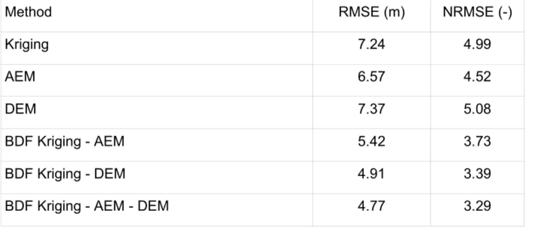
The cross-validation (Fig. 7a) shows that the residuals are centered on zero and, although 375
some outlying residuals show a considerable departure from zero, the root mean squared error 376
is only 7.24 m and the normalized root mean squared error 4.99 %. 377
The RMSE and NRMSE of the calibrated analytical element groundwater model are 378
comparable to the result of kriging (Table 1). The scatterplot of observed vs calculated values 379
(Fig. 7b) however shows that although the number of very large residuals is smaller compared 380
to kriging, the spread of the residuals around zero is larger. In the groundwater level map 381
(Fig. 5c) the difference between the analytic element groundwater model and kriging is 382
clearly visible. The groundwater map shows the draining influence near the rivers and the 383
groundwater mounding due to groundwater recharge in the interfluves. Although the shape of 384
the water table more closely reflects the hydrogeological information available of the aquifer 385
system, locally sizeable differences between observed and calculated groundwater levels 386
exist. 387
The groundwater level estimated by the empirical depth-distance relationship can be 388
considered a subdued replica of topography. On the interfluves, the contour lines are irregular, 389
reflecting variations in the DEM, while the groundwater levels at these locations are expected 390
to be rather smooth and gradually changing. These zones are assigned a high variance, as they 391
have a large penalized distance to the river network. In zones with a low relief, like the 392
alluvial plains and the northern part of the study area, groundwater levels are estimated close 393
to ground surface. The predictive abilities of this empirical model (table 1 and fig. 7c) appear 394
to be only slightly lower than these of kriging interpolation. 395
The first result of Bayesian Data Fusion interpolation is the combination of the kriging 396
interpolation with the estimate from the empirical depth-distance relationship, as already 397
implemented by Fasbender et al. (2008). In the areas with low relief smooth contour lines are 398
produced (Fig. 6a) and the drainage network is incorporated in the interpolation result. On the 399
interfluves however, the contour lines are often highly irregular with numerous small isolated 400
groundwater mounds and depressions. The variance map (Fig. 6b) shows that the zones with 401
high data density and low relief have low variance values. These values increase rapidly 402
however in zones with considerable relief and low data density. The scatterplot of cross-403
validation results (Fig. 7e) and the RMSE value of 4.91m (Table 1) indicate a marked 404
improvement in predictive capability, compared to the individual additional data sources. 405
The BDF interpolation combining kriging with the analytic element groundwater model (Fig. 406
6c), shows a contour map which is similar to the contour map of the analytic element 407
groundwater model (Fig. 5c). The AEM groundwater model however appears to locally 408
overestimate the amount of groundwater mounding in the interfluves. This is remediated in 409
zones with high data density, like around x,y-coordinates (170000,170000), by the higher 410
weight of the kriging in the interpolation. In zones with low data density, the effect of the 411
drainage network on the contour lines of groundwater elevation is clearly apparent. Where 412
data density is high in the vicinity of a river, it is possible that kriging dominates the 413
interpolation as can be seen near x,y-coordinates (145000,150000) and x,y-coordinates 414
(160000,160000). As the AEM groundwater model is characterized by a uniform variance, 415
the variance of BDF of the kriging and AEM (Fig. 6d) is a scaled replica of the kriging 416
variance (Fig. 5b). The RMSE of this interpolation, 5.42 m, is slightly higher than the RMSE 417
of the BDF of kriging and the depth-distance relationship. The main reason for the higher 418
RMSE is the presence of higher residuals for the observations with groundwater levels above 419
100m, while for observations below 100m the BDF of kriging and AEM has lower residuals. 420
The ultimate interpolation combines the three data sources, kriging, depth-distance 421
relationship and AEM groundwater model (Fig. 6e). The general shape of the contour lines is 422
largely influenced by the analytic element model. Locally the influence of the other data 423
sources is apparent, especially in zones with high data density (kriging) and near the river 424
network (depth-distance relationship). The influence of the depth-distance relationship can 425
also been seen on the interfluves through the irregularities in the contour lines, arising from 426
the DEM-fluctuations. The variance of the BDF in Fig. 6f benefits clearly from incorporating 427
the empirical depth-distance relationship. The cross-validation results, i.e. both the scatterplot 428
and the RMSE value, show that the combination of the three data sources has the highest 429
predictive capabilities. 430
Conclusions
431
The water table interpolation methodology introduced by Fasbender et al. (2008), based on 432
the Bayesian Data Fusion framework (Bogaert and Fasbender, 2007), is further extended to 433
incorporate conceptual hydrogeological information through groundwater head calculation 434
based on an analytic element groundwater model. 435
The methodology is applied to a sandy aquifer in Belgium using a limited number of head 436
observations. The Bayesian Data Fusion methodology is used to combine kriging with an 437
estimate of groundwater level by an empirical depth-distance relationship and a groundwater 438
level estimate from an automatically calibrated analytic element model. 439
Combining kriging with the empirical depth-distance relationships produces reliable results in 440
areas with low relief and close to the river network. The estimate in zones scarce of data, 441
farther away from the river network benefits from combining the kriging with the analytic 442
element groundwater model. Combining the three sources of data results in a groundwater 443
level interpolation with a high level of predictive capabilities as shown through the leave-one-444
out cross-validation, albeit that the shape of the contour lines in the interfluves can be 445
debatable by the presence of irregularities arising from contribution of the depth-distance 446
relationship. 447
The interpolation methodology presented and applied in this paper shows that using different 448
sources of data in groundwater interpolation within the Bayesian Data Fusion framework, 449
even with limited data, it is possible to produce an accurate water table contour map 450
incorporating conceptual hydrogeological information. 451
Acknowledgements
452
The authors would like to express their gratitude towards DOV and DGRNE for providing the 453
groundwater level observations for the Flemish and Walloon part of Belgium respectively. 454
The comments of the three anonymous reviewers are highly valued and contributed greatly to 455
the improvement of this paper. 456
References
457
Bakker, M. and V.A. Kelson (2009) Writing analytic element programs in Python. Ground 458
Water 47 (6) 828-834 doi: 10.1111/j.1745-6584.2009.00583.x 459
Bakker, M. and O.D.L. Strack (2003) Analytic elements for multiaquifer flow. Journal of 460
Hydrology 271 (1-4) 119-129 461
Batelaan, O., De Smedt, F. and L. Triest (2003) Regional groundwater discharge: 462
phreatophyte mapping, groundwater modeling and impact analysis of land-use change. 463
Journal of Hydrology 275 (1-2) 86-108 doi: 10.1016/S0022-1694(03)00018-0 464
Bogaert, P. and D. Fasbender (2007), Bayesian data fusion in a spatial prediction context: a 465
general formulation. Stochastic Environmental Research And Risk Assessment 21 (6) 466
695-709, doi: 10.1007/s00477-006-0080-3 467
Bronders, J. and F. De Smedt (1991) Geostatistische analyse van de hydraulische 468
geleidbaarheid van watervoerende lagen in Midden-België. (Geostatistical analysis of 469
hydraulic conductivity of the aquifers in Central Belgium, in Dutch). Water 59 (4) 127-470
132 471
Buchanan, S. and J. Triantafilis (2009) Mapping water table depth using geophysical and 472
environmental variables. Ground Water 47 (1) 80-96, doi: 10.1111/j.1745-473
6584.2008.00490 474
Chilès, J.-P. and P. Delfiner (1999) Geostatistics: modeling spatial uncertainty. Wiley: New 475
York 476
Cools, J., Meyus, Y., Woldeamlak, S. T., Batelaan, O. and F. De Smedt (2006) Large-scale 477
GIS-based hydrogeological modelling of Flanders: a tool for groundwater management. 478
Environmental Geology 50 (8) 1201-1209, doi: 10.1007/s00254-006-0292-3 479
Cressie, N. and C.K. Wikle (2002) Space-time Kalman filter. In: El-Shaarawi, A. H. and W. 480
W. Piegorsch (eds). Encyclopedia of Environmetrics. Vol. 4. 2045-2049. Wiley. 481
Databank Ondergrond Vlaanderen (DOV) (2009) Puntenlaag grondwatermeetnet. (Subsoil 482
Database Flanders, Point layer groundwater observation network, in Dutch) Consulted 483
25 May 2009, at http://dov.vlaanderen.be 484
Diréction Générale des Ressources Naturelles et de l’Environnement (DGRNE) (2009), 485
Banque de données 10-sous. (Database 10-sous, in French) 486
Desbarats, A. J., Logan, C. E., Hinton, M. J. and D.R. Sharpe (2002) On the kriging of water 487
table elevations using collateral information from a digital elevation model. Journal of 488
Hydrology 255 (1-4) 25-38, doi:10.1016/S0022-1694(01)00504-2 489
Ehrendorfer, M. (2007) A review of issues in ensemble-based Kalman filtering. 490
Meteorologische Zeitschrift 16 (6) 795-818, doi:10.1127/0941-2948/2007/0256 491
Fasbender, D., Peeters, L., Bogaert, P. and A. Dassargues (2008) Bayesian data fusion applied 492
to water table spatial mapping. Water Resources Research 44 W12422 493
doi:10.1029/2008WR006921 494
Haitjema, H. M. and S. Mitchell-Bruker (2005) Are water tables a subdued replica of the 495
topography? Ground Water 43 (6) 781-786 doi:10.1111/j.1745-6584.2005.00090 496
Hill, M. C. and Tiedeman, C. R. (2007) Effective groundwater model calibration. Wiley 497
Hunt, R.J. (2006) Groundwater modeling applications using the analytic element method. 498
Ground Water 44 (1) 5-14 doi:10.1111/j.1745-6584.2005.00143.x 499
Huysmans, M., Peeters, L., Moermans, G. and A. Dassargues (2008) Relating small-scale 500
sedimentary structures and permeability in a cross-bedded aquifer. Journal of Hydrology 501
361 (1-2) 41-51, doi:10.1016/j.jhydrol.2008.07.047 502
Karanovic, M, Tonkin, M and D. Wilson (2009) KT3D_H2O: A program for kriging water 503
level data using hydrologic drift terms. Ground Water 47 (4) 580-586 504
doi:10.1111/j.1745-6584.2009.00565.x 505
Kresic, N. (2006) Hydrogeology and groundwater modeling. Second Edition. CRC Press. 506
Laga, P., Louwye, S. and S. Geets (2001) Paleogene and neogene lithostratigraphic units 507
(Belgium). Geologica Belgica 4 (1-2) 135-152 508
Linde, N., Revil, A., Bolève, A., Dagès, C., Castermant, J., Suski, B. and M. Voltz (2007) 509
Estimation of the water table throughout a catchment using self-potential and 510
piezometric data in a Bayesian framework. Journal of Hydrology 334 (1-2) 88-98, 511
doi:10.1016/j.jhydrol.2006.09.027 512
Poeter, E., Hill, M.C., Banta, E., Mehl, S. and S. Christensen (2005) UCODE_2005 and six 513
other computer codes for universal sensitivity analysis, calibration and uncertainty 514
evaluation. US Geological Survey Techniques and Methods 6-A11. 283p. 515
Procter, C., Comber, L., Betson, M., Buckley, D., Frost, A., Lyons, H., Riding, A. and K. 516
Voyce (2006) Identifying crop vulnerability to groundwater abstraction: Modeling and 517
expert knowledge in a GIS. Journal of Environmental Management 81 (3) 296-306, 518
doi:10.1016/j.jenvman.2006.01.016 519
Reilly, T. E. (2001) System and boundary conceptualization in groundwater flow simulation. 520
Techniques of water-resources investigations of the US Geological Survey Book 3, 521
applications of Hydraulics, Chapter B8. US Geological Survey: Virginia 522
Rémy, N. (2004) S-GeMS: Geostatistical Earth Modelling Software: User’s Manual. Stanford 523
University: Stanford 524
Rivest, M., Marcotte, D. and P. Pasquier (2008) Hydraulic head field estimation using kriging 525
with an external drift: A way to consider conceptual model information. Journal of 526
Hydrology 361 (3-4) 349-361, doi:10.1016/j.jhydrol.2008.08.006 527
Strack, O.D.L. (2003) Theory and applications of the analytic element method. Reviews of 528
geophysics 41 (2) 1005 doi:10.1029/2002RG000111 529
Sun, Y., Kang, S., Li, F. and L. Zhang (2009) Comparison of interpolation methods for depth 530
to groundwater and its temporal and spatial variations in the Minqin oasis of northwest 531
China. Environmental Modelling & Software 24 (10) 1163-1170. 532
doi:10.1016/j.envsoft.2009.03.009 533
Taany, R., Tahboub, A. and G. Saffarini (2009) Geostatistical analysis of spatiotemporal 534
variability of groundwater level fluctuations in Amman-Zarqa basin, Jordan: a case 535
study. Environmental Geology 57 (3) 525-535, doi:10.1007/s00254-008-1322-0 536
Tonkin, M. J. and S. P. Larson (2002) Kriging water levels with a regional-linear and point-537
logarithmic drift. Ground Water 40 (2) 185-193, 538
Figure Captions
539
Figure 1: Geological map of the study area (after Cools et al., 2006) 540
Figure 2: Topography of the study area, river network and head observation locations. 541
Figure 3: (a) north-south trend identification from observation data and (b) experimental 542
variogram together with the Gaussian variogram model (nugget: 11m2, sill: 308 m2, 543
range: 11170 m) 544
Figure 4: Graph of groundwater depth DEM(x) - Z(x) as a function of penalized distance 545
dDEM(x) to the network. Dots represent the observed pair of values, solid line 546
represents the fitted nonlinear relationship g(), whereas dashed lines represent the 547
95% symmetric confidence interval based on a Gaussian distribution. 548
Figure 5: (a) kriging interpolation, (b) kriging variance, (c) groundwater levels from the 549
analytic element groundwater model, (d) variance of the analytic element 550
groundwater model, (e) groundwater levels estimated with the empirical depth-551
distance relationship (f) variance of the empirical depth-distance estimated 552
groundwater level 553
Figure 6: (a) BDF of kriging and DEM, (b) variance of BDF of kriging and DEM, (c) BDF of 554
kriging and AEM, (d) variance of BDF of kriging and AEM, (e) BDF of kriging, 555
DEM and AEM, (f) variance of BDF of kriging, DEM and AEM. 556
Figure 7: Cross-validation results. Observed vs calculated values by (a) kriging, (b) analytic 557
element groundwater model, (c) empirical depth-distance relationship, (e) BDF of 558
kriging and AEM, (f) BDF of kriging and DEM, (e) BDF of kriging, AEM and DEM 559
Tables
561
Table 1: Root mean squared error and normalized root mean squared error of cross-validation 562
Method RMSE (m) NRMSE (-)
Kriging 7.24 4.99
AEM 6.57 4.52
DEM 7.37 5.08
BDF Kriging - AEM 5.42 3.73
BDF Kriging - DEM 4.91 3.39
BDF Kriging - AEM - DEM 4.77 3.29