HAL Id: hal-02933268
https://hal.archives-ouvertes.fr/hal-02933268
Submitted on 8 Sep 2020HAL is a multi-disciplinary open access
archive for the deposit and dissemination of sci-entific research documents, whether they are pub-lished or not. The documents may come from teaching and research institutions in France or abroad, or from public or private research centers.
L’archive ouverte pluridisciplinaire HAL, est destinée au dépôt et à la diffusion de documents scientifiques de niveau recherche, publiés ou non, émanant des établissements d’enseignement et de recherche français ou étrangers, des laboratoires publics ou privés.
Bayesian statistical analysis of hydrogeochemical data
using point processes: a new tool for source detection in
multicomponent fluid mixtures
Christophe Reype, Antonin Richard, Madalina Deaconu, Radu S. Stoica
To cite this version:
Christophe Reype, Antonin Richard, Madalina Deaconu, Radu S. Stoica. Bayesian statistical analysis of hydrogeochemical data using point processes: a new tool for source detection in multicomponent fluid mixtures. RING Meeting 2020, Sep 2020, Nancy, France. �hal-02933268�
Bayesian statistical analysis of hydrogeochemical data using point processes: a
new tool for source detection in multicomponent fluid mixtures
C. Reype1, A. Richard2, M. Deaconu1, and R. S. Stoica3
1Universit´e de Lorraine, CNRS, Inria, IECL, F-54000 Nancy, France 2Universit´e de Lorraine, CNRS, GeoRessources, F-54000 Nancy, France
3Universit´e de Lorraine, CNRS, IECL, F-54000 Nancy, France
September 2020
Abstract
Hydrogeochemical data may be seen as a point cloud in a multi-dimensional space. Each dimension of this space represents a hydrogeochemical parameter (i.e. salinity, solute concentration, concentration ratio, isotopic composition...). While the composition of many geological fluids is controlled by mixing between multiple sources, a key question related to hydrogeochemical data set is the detection of the sources. By looking at the hydrogeochemical data as spatial data, this paper presents a new solution to the source detection problem that is based on point processes. Results are shown on simulated and real data from geothermal fluids.
Introduction
The composition of many geological fluids is controlled by variable contributions of multiple sources (e.g. seawater, meteoric water, hydrothermal water). The knowledge of these sources helps to built conceptual and quantitative models of fluid and mass transfer in the Earth’s crust (Yardley & Bodnar, 2014). If the sources are known, the contribution of each sources in every mixture can be inferred from hydrogeochemical data (e.g. Carrera, V´azquez-Su˜n´e, Castillo, & S´anchez-Vila, 2004; Skuce, Longstaffe, Carter, & Potter, 2015). In the case where the sources are not known, they can be inferred from the data (e.g. Pinti et al., 2020).
The paper presents a Bayesian method of source detection based on point processes. The method is inspired by pattern detection methodologies used in image analysis, animal epidemiology and astron-omy (R. Stoica, Descombes, & Zerubia, 2004; R. S. Stoica, Gay, & Kretzschmar, 2007; R. S. Stoica, Martinez, Mateu, & Saar, 2005; R. S. Stoica, Mart´ınez, & Saar, 2007).
1
Materials and methods
Let x = {xi, i = 1, . . . , n} be a set of sources, giving the source position within a multi-dimensional
(in practice two-dimensional) space formed by the hydrogeochemical parameters. A data point d is a mixture of these sources (i.e. it is explained by these sources) if it is a barycenter of these sources as stated in (Faure, 1997) i.e.
d =
n
X
i=1
γixi (1)
with 0 ≤ γi≤ 1 for each i and Pni=1γi= 1.
In the Euclidean plane, the source pattern (i.e. set of sources) is unknown and also somehow outlined by the set of hydrogeological data points. The key hypothesis at the basis of our work is that this pattern is made of interacting points. A preliminary condition for our model is that the hidden sources pattern exhibits the following properties :
• two sources cannot be too close
• the data points originating from a mixture of sources should be rather close to them
• the convex hull enclosing the set of data points is enclosed within the convex hull given by the source positions.
These hypotheses allow to consider the sources as a realisation of a point process described by a Gibbs probability density:
p(x|θ) = exp [−U (x|θ)]
Z(θ) =
exp [−Ud(x|θ) − Ui(x|θ)]
Z(θ)
with x the configuration of sources (or set of sources), Z(θ) the normalising constant and U the energy function.
The energy function is built as the sum of two components. The first term, Ud(x|θ) is the data
term and it controls the positioning of the sources with respect to the observed data points d = {d1, d2, . . . , dm}. Its expression is given by
Ud(x, θ) = θ1g(x, d) + θ2 m
X
j=1
α(dj, x) + θ3ne(x, d).
Here g(x, d) is the absolute value difference between the area of the sources and the data point convex hull, respectively. The function α(dj, x) represents the minimum distance between the data point dj
and the sources cloud and it is given by min{kdj − xik22 : i = 1, . . . , n(x)}, with n(x) the number
of sources in the configurations. The measure ne(x, d) counts the number of data points in d, that
belong to the convex hull given by x. The parameters θ1, θ2 ≥ 0 and θ3 ≤ 0 are chosen such that to
penalize important differences between the convex hull areas, to encourage the source to be situated rather close to the data points and to increase the number of data points that are explained by the sources, respectively.
The second term, Ui(x|θ) is the interaction term and it writes as
Ui(x, θ) = θ4n(x) + θ5nr(x).
with nr(x) the number of pairs of sources at distance shorter than r, which is a pre-fixed known value.
The parameters θ4, θ5 ≥ 0 are chosen in order to penalize a too high number of sources and pairs of
sources situated too close, respectively.
The point process on a finite domain W (i.e. µ(W ) =RWξ dξ < ∞), that is defined by the previous energy function, is well defined and locally stable R. Stoica (2014). Based on these terms, the model is able to generate point configurations that exhibit the properties required by the assumed hypotheses. The source pattern is estimated by the point configuration that maximises the probability density p(x|θ)
b
x = arg maxx∈Ωp(x|θ) = arg minx∈ΩU (x|θ). (2)
The solution of the problem (2) is obtained by implementing a simulated annealing algorithm. This algorithm is a global optimisation method that iteratively samples from p(x|θ)1/T while making T → 0 slowly. Convergence properties of this algorithm are shown in R. S. Stoica, Gregori, and Mateu (2005). 1.1 Optimisation algorithm
The implemented simulated annealing algorithm has the following structure: 1) set θ, T , kmax, x(0), c and k = 1
2) while k ≤ kmax
Bayesian analysis of geological data using point processes C. Reype et al.
a) generate x(k) with probability p(x(k−1)|θ)1/T
b) set T = c ∗ T and k = k + 1 3) set x = x(k)
This structure implements a sub-optimal cooling schedule, for practical reasons. An optimal loga-rithmic cooling schedule as specified by R. S. Stoica, Gregori, and Mateu (2005) may be considered.
The sampling of p(x|θ) is done via the Metropolis-Hasting algorithm described below : 1) set rc, pb, pd, pc with pb+ pd+ pc≤ 1
2) with probability pb choose birth, with probability pdchoose death and with probability pcchoose
change.
birth: a) generate a random point η on W and set x0 = x ∪ {η} b) calculate βb = min{1,ppd b p(x∪{η}|θ) p(x|θ) µ(W ) n(x)+1}
death: a) choose a point η of x and set x0 = x \ {η} b) calculate βd= min{1,ppdbp(x\{η}|θ)p(x|θ) µ(W )n(x)}
change: a) choose a point η of x and generate a random point ξ in the ball B(η, rc) and set
x0 = x \ {η} ∪ {ξ}
b) calculate βc= min{1,p(x\{η}∪{ξ}|θ)p(x|θ) }
3) the new configuration x = x0 is accepted with the appropriate probability β ; otherwise the algorithm remains in the same state x.
The previous dynamic is φ− irreducible, Harris recurrent and geometric ergodic, guaranteeing the convergence of the algorithm towards the distribution of interest given by p(x|θ) Moller and Waagepetersen (2003); R. Stoica (2014); van Lieshout (2000).
2
Results
The proposed model was tested on two different data sets. The first one is a simulated data set, the second one is a set of hydrogeochemical data from geothermal fluids described in (Pinti et al., 2020). The model is coded in C++, and the results are displayed in R with the library ”ggplot”.
We set T = 1000, kmax = 10000, c = 0.995, rc = 0.3, pb = 0.35, pd = 0.35 and pc = 0.3. The
parameters θ were chosen separately, for each data set, after several trials and errors. 2.1 Simulated data
The data are created by generating three sources. The vector of contributions of each sources to a data point is generated by a Dirichlet law with parameters (1, 1, 1). Hence the data points are points uniformly distributed in the convex hull given by the sources positions in the 2D space of hydrogeochemical parameters. Moreover, a Gaussian noise, of mean 0 and variance 10−1 for each coordinate, was added to each datapoint to represent the noise during the measurement.
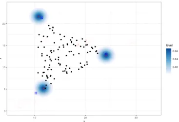
We set the parameters to θ = (100, 1, −100, 700, 50) and r = 2. The results are shown in Figure 1. The black dots are the data points, the blue symbols are the real sources and the gradient of blue color shows the density of simulated sources.
There are three areas that exhibit a high density of simulated sources, which corresponds to the actual number of sources. Moreover their positions are really close to the real sources.
Figure 1: Point process source detection for the simulated data in the case of a three-component fluid mixing system where x and y are the concentrations of two solutes (arbitrary
units)
2.2 Real data
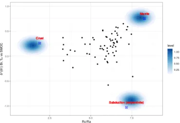
We are now comparing the results of our model with the results of the model presented in (Pinti et al., 2020). This model gives the smallest triangle (in term of area) that enclose the data. In Figure 2 we set θ = (200, 1, −1200, 210, 5), and in Figure 3 we set θ = (196, 2, −1200, 220, 5). The parameters are completely different than in 1 because the data are not in the same scale.
Figure 2: Point process source detection for a three-component geothermal fluid mixing system where δ37Cl, o/oovs SMOC and Rc/Ra are respectively the stable isotopic composition of
chlorine and the4He/3He ratio of the samples (data from (Pinti et al., 2020, Figure 4))
The model is able to detect the number and the position of the sources inferred in (Pinti et al., 2020), while the model sufficient statistics provides a more complete morpho-statistical description of the sources.
3
Conclusions and perspectives
Clearly, the use of this method requires at least partial knowledge regarding the model parameters. Such a knowledge is built by embedding the available geological information into prior distributions.
This new tool should be improved in order to become helpful not only in the analysis of geological
Bayesian analysis of geological data using point processes C. Reype et al.
Figure 3: Point process source detection for a three-component geothermal fluid mixing system where δ81Br, o/oovs SMOB and Rc/Ra are respectively the stable isotopic composition of
bromine and the4He/3He ratio of the samples (data from (Pinti et al., 2020, Figure 5))
fluids but also in other fields that deals with mixtures (e.g. Longman et al., 2018; Phillips & Gregg, 2003). This is possible due to the use of the embedded spatial and Bayesian paradigms.
Acknowledgments
This work was performed in the frame of the DEEPSURF project ( http://lue.univ-lorraine.fr/fr/impact-deepsurf ) at Universit´e de Lorraine. This work was supported partly by the french PIA project Lorraine Universit´e d’Excellence, reference ANR-15-IDEX-04-LUE.
References
Carrera, J., V´azquez-Su˜n´e, E., Castillo, O., & S´anchez-Vila, X. (2004). A methodology to compute mixing ratios with uncertain end-members. Water resources research, 40 (12).
Faure, G. (1997). Principles and applications of geochemistry (Vol. 625). Prentice Hall New Jersey, United States,.
Longman, J., Veres, D., Ersek, V., Phillips, D. L., Chauvel, C., & Tamas, C. G. (2018). Quantitative assessment of pb sources in isotopic mixtures using a bayesian mixing model. Scientific reports, 8 (1), 6154.
Moller, J., & Waagepetersen, R. P. (2003). Statistical inference and simulation for spatial point processes. Chapman and Hall/CRC.
Phillips, D. L., & Gregg, J. W. (2003). Source partitioning using stable isotopes: coping with too many sources. Oecologia, 136 (2), 261–269.
Pinti, D. L., Shouakar-Stash, O., Castro, M. C., Lopez-Hern´andez, A., Hall, C. M., Rocher, O., . . . Ram´ırez-Montes, M. (2020). The bromine and chlorine isotopic composition of the mantle as revealed by deep geothermal fluids. Geochimica et Cosmochimica Acta.
Skuce, M., Longstaffe, F., Carter, T., & Potter, J. (2015). Isotopic fingerprinting of groundwaters in southwestern ontario: Applications to abandoned well remediation. Applied Geochemistry, 58 , 1–13.
Stoica, R. (2014). Mod´elisation probabiliste et inf´erence statistique pour lanalyse des donn´ees spa-tialis´ees. Research Habilitation Thesis, Universit´e Lille, 1 .
Stoica, R., Descombes, X., & Zerubia, J. (2004). A gibbs point process for road extraction from remotely sensed images. International Journal of Computer Vision, 57 (2), 121–136.
Stoica, R. S., Gay, E., & Kretzschmar, A. (2007). Cluster pattern detection in spatial data based on monte carlo inference. Biometrical Journal: Journal of Mathematical Methods in Biosciences, 49 (4), 505–519.
Stoica, R. S., Gregori, P., & Mateu, J. (2005). Simulated annealing and object point processes : tools for analysis of spatial patterns. Stochastic Processes and their Applications, 115 , 1860-1882. Stoica, R. S., Martinez, V. J., Mateu, J., & Saar, E. (2005). Detection of cosmic filaments using the
candy model. Astronomy & Astrophysics, 434 (2), 423–432.
Stoica, R. S., Mart´ınez, V. J., & Saar, E. (2007). A three-dimensional object point process for detection of cosmic filaments. Journal of the Royal Statistical Society: Series C (Applied Statistics), 56 (4), 459–477.
van Lieshout, M. N. M. (2000). Markov point processes and their applications. Imperial College Press, London.
Yardley, B. W., & Bodnar, R. J. (2014). Fluids in the continental crust. Geochemical Perspectives, 3 (1), 1–2.
Bayesian analysis of geological data using point processes C. Reype et al.