HAL Id: hal-01580622
https://hal.archives-ouvertes.fr/hal-01580622
Submitted on 1 Sep 2017
HAL is a multi-disciplinary open access
archive for the deposit and dissemination of
sci-entific research documents, whether they are
pub-lished or not. The documents may come from
teaching and research institutions in France or
abroad, or from public or private research centers.
L’archive ouverte pluridisciplinaire HAL, est
destinée au dépôt et à la diffusion de documents
scientifiques de niveau recherche, publiés ou non,
émanant des établissements d’enseignement et de
recherche français ou étrangers, des laboratoires
publics ou privés.
Optimize Wireless Networks for Energy Saving by
Distributed Computation of Čech Complex
Ngoc-Khuyen Le, Anais Vergne, Philippe Martins, Laurent Decreusefond
To cite this version:
Ngoc-Khuyen Le, Anais Vergne, Philippe Martins, Laurent Decreusefond. Optimize Wireless Networks
for Energy Saving by Distributed Computation of Čech Complex. The 13th IEEE International
Conference on Wireless and Mobile Computing, Networking and Communications, WiMob 2017, 2017,
Roma, Italy. �hal-01580622�
Optimize Wireless Networks for Energy Saving
by Distributed Computation of ˇ
Cech Complex
Ngoc-Khuyen Le, Ana¨ıs Vergne, Philippe Martins, Laurent Decreusefond
LTCI, CNRS, T´el´ecom ParisTech, Universit´e Paris-Saclay, 75013, Paris, France
Email:{ngoc-khuyen.le, anais.vergne, philippe.martins, laurent.decreusefond}@telecom-paristech.fr
Abstract—In this paper, we introduce a distributed algorithm to compute the ˇCech complex. This algorithm is aimed at solving the coverage problems in self organized wireless networks. The complexity to compute the minimal ˇCech complex that gives information about coverage and connectivity of the network is O(n2), where n is the average number of neighbors of each
cell. An application based on the distributed computation of the ˇCech complex, which is aimed at optimizing the wireless network for energy saving, is also proposed. This application also has polynomial complexity. The performance of the proposed algorithm and its application are evaluated. The simulation results show that the distributed computation of the ˇCech complex provides a consistent outcome with the one obtained by the centralized computation that is introduced in [6], while requires a much shorter calculation time. The optimized coverage saves 65% of the total transmission power, while also keeps the maximal coverage for the network.
I. INTRODUCTION
Coverage is a key factor that determines the quality of service in wireless networks. In recent applications to solve coverage problems in wireless networks, simplicial complex is often utilized to represent the network topology. Unlike graph, which represents only the neighborhood of cells, sim-plicial complex represents the topology of cells with a higher dimension.
The ˇCech complex is a simplicial complex that represents a collection of cells by a simplex if they have a non-empty in-tersection. The ˇCech complex represents exactly the topology of the network [3]. For this reason, the ˇCech complex is the right tool to describe and optimize the coverage for wireless networks. In [2], an algorithm to compute the ˇCech complex is introduced, but this algorithm is designed to be utilized in graphics science, and it only works with a collection of cells that have the same size. Nowadays, the wireless networks are becoming more and more dense and heterogeneous. This algorithm is not suitable to represent these networks. Although an algorithm to compute the ˇCech complex for a collection of cells that have different sizes is proposed in [6], this algorithm is still centralized. It is not suitable to represent future wireless networks, which should be self-organized.
In [7], authors use the ˇCech complex to optimize the cov-erage for wireless networks. As the computation of the ˇCech complex is only available in centralized way, this application is not distributed. In [5], [9], some algorithms based on simplicial homology are developed to detect coverage holes in wireless networks. Although these algorithms are available in both
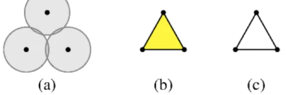
centralized and distributed ways, they use the Rips complex instead of the ˇCech complex to represent the topology of the network. However, the Rips complex is still an approximation of the ˇCech complex. In fact, the Rips complex represents a collection of cells by a simplex if every pair of cells in this collection are intersected (or they are neighbors). Therefore, the Rips complex may not capture exactly the topology of the network. So, some coverage holes may be undiscovered, see Figure 1 for an example. In this figure, a coverage hole inside three cells is represented by an empty triangle (not a 2-simplex) in the ˇCech representation. It indicates that there is a hole inside three edges of the triangle. However, any pair of cells are intersected so the Rips complex represents these cells by a filled triangle (a 2-simplex). It means that no coverage hole is presented in the Rips representation. The ˇCech complex represents exactly the coverage hole, but the Rips complex does not.
Fig. 1: (a) Cells, (b) Rips complex, (c) ˇCech complex. In this paper, we introduce a distributed algorithm to compute the ˇCech complex for a given collection of cells that have different sizes. This algorithm is developed for solving coverage problems in self-organized wireless net-works. The computation of the minimal ˇCech complex, which gives information about the coverage and connectivity of the network, is only O(n2), where n is the average number
of neighbors of each cell. Following the simulation results, our distributed computation of the ˇCech complex provides a consistent outcome with the one obtained by the centralized computation that is introduced in [6], while requires much shorter computation time.
An example of the network deployment and its representa-tion by the ˇCech complex is shown in Figure 2. The network in Figure 2a contains cells whose sizes are various. The center of each cell is marked as a black point. The covering domain of each cell is drawn in gray. In Figure 2b, every two neighbor cells are connected by a black edge (1-simplex). Each 2-simplex is represented by a yellow triangle. Each 3-2-simplex is drawn as a green tetrahedron, which represents the common
intersection of 4 cells. The 4-simplices, which have the highest dimension, are drawn in red. The red areas present the most overlapped regions. The region that is not colored indicates a coverage hole.
(a) A random deployment of cells (b) ˇCech complex
Fig. 2: An example of the deployment of cells and its ˇCech complex
We also propose an application that is based on the dis-tributed computation of the ˇCech complex. Given a random deployment of a wireless network, this application optimizes the coverage of the network. The optimized coverage reduces as much as possible the intersections among cells. As a result, the waste power due to interference within intersected regions is avoided efficiently. The total transmission power is reduced while the maximal coverage of the network is conserved. Our simulation results show that the optimized coverage saves 65% of the total transmission power in dense network. This application is also distributed and has only polynomial complexity.
This paper is organized as follows. Section II introduces a short background of simplicial homology and its applications in wireless networks. Section III describes all details about the distributed computation of the ˇCech complex. Section IV proposes a distributed coverage optimization algorithm aimed at energy saving for wireless networks. Section V shows our simulations and results. The last section concludes our paper with discussions and directions for future works.
II. SIMPLICIAL HOMOLOGY
This section introduces some notions of algebraic topology, and also explains how they can be used to capture and analyze the topology of the network. For more details about algebraic topology, see [8].
A. Simplicial complex
Let Sk = {v0, v1, . . . , vk} be a set of k + 1 geometrically
independent points in Rn, where n > k. The convex hull
ofS is defined as a k-simplex, denoted by sk, wherek is its
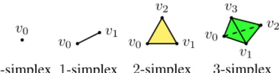
dimension andv0, v1, . . . , vkare its vertices. Thus, a 0-simplex
is a single point, an 1 -simplex is an edge, a 2-simplex is a triangle, a 3-simplex is a tetrahedron, and so on. See Figure 3 for some instances.
The convex hull of any subset of Sk, which is also
geo-metrically independent, is a lower dimensional simplex. This
v0 0-simplex 1-simplex v0 v1 2-simplex v0 v1 v2 3-simplex v0 v1 v2 v3
Fig. 3: An example of simplices.
simplex is called al-face of skifl is its dimension. An abstract
simplicial complex is a collection of simplices such that: every face of any simplex in this collection is also in this collection.
B. Homology group
We define the orientation of a simplex as an order of its vertices. A simplex {v0, v1, . . . , vk} considering the order
of its vertices is called an oriented simplex, denoted by [vo, v1, . . . , vk]. If the vertices of a simplex is transformed by
an odd permutation, its orientation changes into the inverse one. If two vertices of a simplex swap their positions, then the orientation of this simplex is reversed, and denoted by the negative sign as:
[v0, . . . , vi, . . . , vj, . . . , vk] = −[v0, . . . , vj, . . . , vi, . . . , vk].
Given K an abstract simplicial complex, the k-chain group Ck(K) is the vector space spanned by the set of oriented
k-simplices of K. The boundary operator ∂k is defined as the
linear transformation∂k : Ck(K) → Ck−1(K) which acts on
basis elements[v0, v1, . . . , vk] via:
∂k[v0, v1, . . . , vk] = k
X
i=0
(−1)i[v0, v1, . . . , vi−1, vi+1, . . . , vk],
where[v0, v1, . . . , vi−1, vi+1, . . . , vk] is the i-th face obtained
by deleting thei-th vertex from [v0, v1, . . . , vk]. The boundary
of ak-simplex is its collection of (k − 1)-faces. It is simple to verify that∂k◦ ∂k+1= 0. This result means that the boundary
of every chain has no boundary. Ak-chain is called a k-cycle if its boundary is zero. So, the group ofk-cycles, denoted by Zk(K), is the kernel of ∂k: Ck(K) → Ck−1(K). The group
ofk-boundaries, denoted by Bk(K), is the image of ∂k+1 :
Ck+1(K) → Ck(K). Since ∂k◦∂k+1= 0 for every k, each
k-boundary is automatically ak-cycle. It implies that Bk(K) ⊂
Zk(K) for all k. We now define the k-th homology group of
K as the quotient vector space: Hk(K) = Zk(K)/Bk(K).
The dimension of Hk is called thek-th Betti number:
βk = dim Hk = dim Zk− dim Bk. (1)
The Betti number has an important meaning in solving cov-erage problems. Given a simplicial complex that presents the coverage of a network, its k-th Betti number βk counts
the k-dimensional holes. For example, while the connected components are counted byβ0, the coverage holes are counted
β1. Therefore, if β0 = 1, the network is connected. There is
no coverage hole ifβ1= 0.
C. Simplicial complex of cellular networks
Definition 1 ( ˇCech complex): Given a collection of cover sets U, the ˇCech complex of U, denoted as ˇC(U), is the
abstract simplicial complex whose k-simplices correspond to nonempty intersection ofk + 1 distinct elements of U.
If each cover set in the collectionU is the coverage of a cell in the wireless network, then the ˇCech complex ofU captures exactly the topology of this network [3].
III. DISTRIBUTED COMPUTATION OFCˇECH COMPLEX
A. System model
We consider a wireless network composed of N distinct cells. We assume that each cell uses isotropic propagation. The coverage of the i-th cell is modeled as:
ci(vi, ri) = {z ∈ R2: kz − vik ≤ ri},
where k.k is the Euclidean distance, the vertex vi represents
the base station location and ri is the coverage radius of the
i-th cell. Let U be the collection of cells, then U = {ci, for i =
0, 1, . . . , (N − 1)}. The ˇCech complex ofU, ˇC(U), is defined as the ˇCech complex of the wireless network. In the ˇCech complex, each vertex, i.e. a 0-simplex, vi corresponds to
the i-th cell ci in the network. An edge, i.e. a 1-simplex,
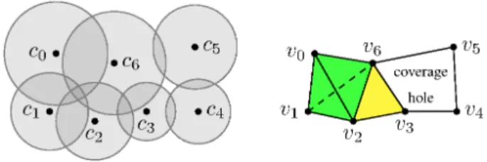
represents the connection, or the intersection, between two cells. Each k-simplex, where k ≥ 2, represents the common intersection of the coverage of together(k + 1) corresponding cells of this simplex. For example, in Figure 4, the 2-simplex [v2, v3, v6] means the overlap of coverage of cell c2, cell c3
and cell c6. There is no coverage hole inside these cells. The
higher dimension of the simplex is, the higher number of overlaps is. The 3-simplex[v0, v1, v2, v6] means that the four
corresponding cells:c0,c1,c2andc6, together, have a common
intersection. In contrast, a chain of 1-simplices indicates a coverage hole inside corresponding cells of the chain. For example, the chain[v3, v4] + [v4, v5] + [v5, v6] + [v6, v3] covers
a coverage hole inside four cellsc3,c4,c5andc6. To analyze
the network topology, we use characteristics of the homology of the ˇCech complex.
Fig. 4: Cells and their ˇCech representation.
B. Distributed computation of the ˇCech complex
In this subsection, we describe all the details about how each cell can cooperate with others to construct the ˇCech complex. We denote Sk the collection of all k-simplices of
the complex. As the definition of the ˇCech complex, each k-simplex represents the common intersection of together its (k + 1) corresponding cells. Each vertex, that is a 0-simplex, corresponds to a cell of the network. The collection of 0-simplices, S0, is then obviously the list of corresponding
vertices of cells.
S0= {vi| i = 0, 1, . . . , (N − 1)}.
If a group of cells form ak-simplex, where k ≥ 1, then every pair of cells in this group are neighbors. So, each cell needs to detect all its neighbors before computing the simplices.
1) Neighbors detection: We assume that each cell ci can
communicate with other cells over radio within a distance Di= 2ri. We assume that there are enough frequency slots for
cells to communicate over radio without collision. Every cell is also connected by a backhaul network. At the initial state, each cell broadcasts a probe message with its position and its radius over radio channel. If a cell receives a probe message, it verifies if the cell that sent this probe message is a neighbor. Two cells are neighbors if they are intersected. If they are neighbors, then the cell that received the probe message sends a relationship confirmation together with its position and its radius to the cell that sent the probe message by using the backhaul network. After receiving the confirmation, the cell that sent the probe message adds the cell that sent the confirmation into its collection of neighbors.
If two cellsa and b are neighbors, the distance between them isd(a, b) ≤ ra+ rb. Let us assume thata is the bigger cell,
so ra ≥ rb, thend(a, b) ≤ 2ra which is the communication
distanceDaof the cella. So, the smaller cell b always receives
the probe message from the bigger cella. Therefore, if there are two cells that are neighbors, the neighborhood is always detected by the smaller cell. We assume that all the cells can reply the confirmation within a periodtack. After this period
tack, every cell detects its collection of neighbors. We denote
the collection of neighbors of the cellci as Ni.
2) Distributed simplices computation: When the collection of neighbors is available, each cell computes its simplices by verifying the intersection among it and its neighbors. As each pair of neighbors form a simplex, the collection of 1-simplices of each cellci is easily found:
S1,i= {[vi, vj] | cj∈ Ni}.
To find allk-simplices, where k ≥ 2, each cell verifies if a group of it and its k neighbors has a common intersection. If these cells have a common intersection, then this group forms ak-simplex.
We now consider a group of(k + 1) cells and verify if they form ak-simplex. Let us denote ˆcl(ˆvl, ˆrl) the considered cell in
this group, wherel = 0, 1, . . . , k. The collection of vertices of these cells ˆsk = [ˆv0, ˆv1, . . . , ˆvk] is considered as a candidate
to be a k-simplex. To decide if this ˆsk is a k-simplex, we
now need to verify if all these corresponding cellscˆl, where
l = 0, 1, . . . , k, have a common intersection.
Let us assume that sˆk is a k-simplex. It means that there
is a common intersection of all these corresponding cells. We denote I to be this intersection, we have:
I= ∩ˆcl, for l = 0, 1, . . . , k.
Let p be a point that belongs to I, then p must belong to all corresponding cells cˆl, where l = 0, 1, . . . , k. We denote
circle ˆbl the boundary, or the cover, of the cellˆcl, and X the
collection of intersection points of every pair of these circles. X= {ˆbm∩ ˆbn| 0 ≤ m < n ≤ k}.
There are only two possible cases:
• The first case: X∩ I = ∅. There is no intersection point that belongs to I. In this case, the smallest circle, ˆbmin=
min {ˆbl| l = 0, 1, . . . , k}, must be inside all other circles
ˆbl that ˆbl6= ˆbmin. See an example in Figure 5.
Fig. 5: The smallest cell is inside the other cells.
• The second case: X∩ I 6= ∅. There must exist two
circles ˆbm and ˆbn (the boundary of cˆm and ˆcn), that at
least one of their intersection points belongs to all other corresponding cellsˆcl, where l 6= m and l 6= n. See an
example in Figure 6.
Fig. 6: There is a pair of cells whose one intersection point (the red point) is inside the other cells.
So, to verify a candidate to be ak-simplex, we need to verify if it satisfies one of these two cases above. If this candidate does not satisfy both of these two cases above, then it is not ak-simplex. See an example in Figure 7.
Fig. 7: The smallest cell is not inside the other cells, and no intersection point of any pair of two cells is inside the other cells.
However, neighborhood is a two-way relationship. There-fore, the verification of intersection could be duplicated by different cells that are neighbors. To avoid the redundant duplication, each cell verifies the intersection by following a right hand rule. This rule is that each cell verifies only with neighbors that are on its right hand side. If there is a neighbor which has the same horizontal coordinate, it verifies only this neighbor if it has higher vertical coordinate. If a simplex is found by a cell, this cell transmits this simplex to every cell that belongs to this simplex. As a result, every cell detects all
its simplices. For example, in Figure 4, the cellc2verifies the
intersection with only the cellc3andc6. It detects the simplex
[v2, v3, v6]. It receives its other simplices from the neighbor c0
andc1. The Algorithm 1 reports the distributed computation
of ˇCech complex for each cell. In this algorithm, we denote ci the cell that is computing the simplices and (xi, yi) its
coordinates. The parameter “count time” counts time up from Algorithm 1 Distributed computation of ˇCech complex Input: ci the cell that is computing;
Output: ˇCi the collection of simplices of the cellci; broadcast{probe, vi,ri} over radio;
S0= vi;
count time= 0;
while count time< tackdo
if{probe, vj,rj} is received from cj then
ifd(vi, vj) < ri+ rj then addvj to Ni; ifxi< xj then addvj to S0; add[vi, vj] to S1; end if ifxi== xj andyi < yj then addvj to S0; add[vi, vj] to S1; end if end if end if
update count time; end while
S′
0= S0/vi;
fork = 2 to dimmax do
forl = 2 to Ck |S′ 0| do ˆ s = l-th combination of k vertices in S′ 0; ˆ s = ˆs ∪ {vi}; ˆ c = corresponding cells of ˆs;
if intersection of all cells inc is not empty thenˆ addˆs to Sk; end if end for end for ˇ Ci= {S0, S1, . . . , Sk};
send ˇCi to every corresponding cell of vertices in S0;
ni= |Ni|;
whileni> 0 do
if ˇCj is received fromcj in Ni/S0 then
ˇ Ci= ˇCi∪ ˇCj; ni= ni− 1; end if end while return ˇCi;
the moment the cell ci broadcasts the probe message. The
highest dimension of simplices that are considered is dimmax.
The output of this algorithm, the collection of simplices of the cellci is denoted as ˇCi.
The global ˇCech complex that represents the topology of the whole network is sometimes needed. There should be a master cell that controls the topology of the network. This global ˇCech complex ˇC(U) can be easily built by integrating the simplices computed from every cell as:
ˇ
C(U) = ∪N−1
i=0 Cˇi.
Each cell sends its computed simplices that contain only the vertices satisfied the right hand rule. One more time, this rule is useful as it avoids sending the duplicated simplices.
C. Complexity
We denote the average number of neighbors of each cell by n. To find a k-simplex, each cell needs to verify the common intersection of a group of it and its k neighbors. To find all k-simplices, the number of groups to verify is Ck
n. So, to find
all k-simplices for 1 ≤ k ≤ dmax, the number of groups to
verify isPdmax
k=1C k n.
If we consider only the connectivity and coverage of the wireless network, the ˇCech complex built up to dimension two is enough. In this case, the complexity to find all simplices up to dimension two of each cell is O(n2). If we consider the
ˇ
Cech complex with the highest dimensiondmax, assuming that
dmax= ∞, the sumPdk=1max Cnk is upper bounded by2n. So, the
complexity to find all the simplices up to the highest dimension is O(2n). Although it is not polynomial, the term 2n is not
tremendous because the average number of neighbors of each cell is normally not so big. The complexity of our distributed construction of the ˇCech complex is much smaller than the one of the centralized construction proposed in [6]. The complexity to build the ˇCech complex up to dimension two and up to its highest dimension by the centralized construction areO(N2
+ N n2
) and O(N2
+ N 2n), respectively.
IV. COVERAGE OPTIMIZATION FORENERGYSAVING
One application of the distributed computation of the ˇCech complex is coverage optimization for energy saving in wireless networks. Our proposal jointly maximizes its coverage and minimizes its total transmission power. Firstly, we ensure a maximal coverage for the network. Each cell is turned on and is set to work with the highest transmission power. At this initial state, the network has the largest coverage. However, many cells are hardly overlapped. The overlapping region between cells causes the waste of transmission power due to interference. We can optimize the transmission power by reducing the overlapping regions. However, the global coverage of the network should be conserved. In other words, the two Betti numbers β0 andβ1 of the ˇCech complex of the
network should be kept unmodified. The transmission power of each cell is estimated following the simplified path loss model:
Pt,i= K0r γ
i, (2)
whereK0is a constant factor andγ is the path loss exponent.
In this paper,K0 is assumed to be 1 for simplification. The
optimization problem can be written as:
min r N−1X i=0 rγi s.t. β0= β∗0 β1= β∗1 r = (r0, r1, . . . , rN−1), (3) whereβ∗
0 andβ1∗ are the Betti numbers of the ˇCech complex
of the network at the initial state.
We introduce a distributed algorithm to optimize the cover-age as well as to save energy for the network. This algorithm is applied for each cell in the network. We assume that all the fenced cells and boundary cells are already known. Only the cells that are not fenced or boundary cells can try to reduce the coverage radius. We assume that each cell ci in the network can be active with a coverage radius ri,
where ri,min ≤ ri ≤ ri,min. If after the optimization process
ri≤ ri,min, the cellciis turned off. We also assume that every
cell is connected to each other by a backhaul network. At the first step, each cell needs to search for its neighbors as well as its simplices by following the Algorithm 1. Once the neighbors set is established, each cell starts its reduction process. On each cell, there is a timer which counts down to zero. The timer is set to a uniform random value from 1 to tmax, wheretmax is the maximal value of the timer. When the
timer of a cell is expired, this cell tries to do a reduction. If two cells that are neighbors try to reduce their radius at the same time, the coverage hole may not be detected due to the outdated information about the radius of each other. Therefore, before trying to reduce the radius, each cell sends a “pause” message to its neighbors. Then, the cell reduces its coverage radius and verifies the coverage.
Algorithm 2 Coverage verification after a radius reduction of one cell
Input:
c∗ the cell that changed its radius;
N = neighbors collection of the cell c∗;
ˇ
C∗ = the ˇCech complex of{c∗} ∪ N before the radius reduction;
Output: true if and only if there is no new coverage hole. compute Betti numbersβ∗
0 andβ1∗ of ˇC∗;
ˇ
C = the ˇCech complex of {c∗} ∪ N after the radius
reduction;
compute Betti numbersβ0 andβ1 of ˇC;
ifβ0= β0∗ andβ1= β1∗ then verification = true; else verification = false; end if return verification;
The radius reduction of one cell only makes topology change in the local region that is comprised of this cell and
its neighbors. If there is a new coverage hole, it must be inside this local region. This means that if there is no new coverage hole after the radius reduction, the Betti numbersβ0
andβ1of the ˇCech complex of this local region are unchanged.
The verification of the network coverage can be reduced to the coverage verification in only this local region as in the Algorithm 2.
If no hole appears, the cell confirms the reduction and sends the new value of coverage radius to its neighbors. It also sends the “continue” message to its neighbors to tell them that they can continue. If a cell received a “pause” message, it pauses its process and waits until the message “continue” is received. Then, it continues its process normally.
Algorithm 3 Distributed energy saving algorithm for each cell Input: c a cell in the network;
Output: the optimal radius forc;
transmit the position and the coverage radius of c to other cells;
collect the information about the position and coverage of other cells;
while (1) do
set timer = uniform(0, tmax);
wait until timer expires;
Nc= the collection of neighbors of c;
if a “pause” received then wait until “continue” received; end if
rold= rc;
rc= rc− ∆rc;
if rc < rc,min then
rc= 0;
verify the coverage;
if no coverage hole appears then
transmit the “turning off” to other cells; send “continue” to neighbors in Nc;
else rc= rold;
send “continue” to neighbors in Nc;
end if break; else
verify the coverage;
if no coverage hole appears then send rc to neighbors inNc;
send “continue” to neighbors in Nc;
else rc= rold;
send “continue” to neighbors in Nc;
break; end if end if end while return;
There is a special case where two neighbor cells whose
timers expire at the same time send the “pause” message to each other simultaneously. One of these two cells receives a “pause” from another before it sends “continue” message to other cells. This cell cancels the current reduction step and sets a new value for its timer and waits to retry.
If a cell tries to reduce its coverage radius and makes a coverage hole, it reverses its coverage radius to the previous value and stops the reduction process. This cell is set to irreducible.
The distributed energy saving algorithm applied for each cell is described in the Algorithm 3. The main step in this algorithm is to verify the coverage of the local region. This step requires the computation of the ˇCech up to dimension 2 and its Betti numbersβ0, β1. The computation of this ˇCech
complex has complexity O(n2). The computation of the two
Betti numbersβ0 andβ1 are based on the rank computation
of the homology space of the ˇCech complex. The complexity of these computations are discussed in [4]. Let we denote mk the average number ofk-simplices of the ˇCech complex.
The computation of β0 has the complexity of O(m1). The
complexity of the computation ofβ1is equal to the complexity
of the rank computation of a square matrix m2 rows and
m2 columns, which is O(m32). The number of k-simplices
in the ˇCech complex can be upper bounded by Cn+1k+1. So,
the complexity to compute both these two Betti numbersβ0
and β1 is then as much O(n9). It is much smaller than the
complexities of the centralized energy saving algorithm and the simulated annealing algorithm, which are O(N4n6) and
O(KLN3n6), respectively [7]. In these terms, N is much
bigger than n. The number K and L are parameters of temperature schedule, which are set to a great value for a good approximation of the global optimum solution [1].
V. SIMULATION AND RESULTS
A. Performance of the distributed computation of the ˇCech complex
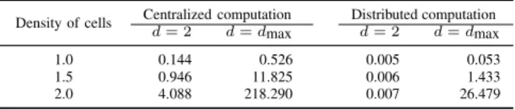
We compare the performance of our distributed construction of the ˇCech complex with the centralized one which is proposed in [6]. Cells are randomly deployed according to the Poisson point process on a square [30 × 5]. The density of cells is varied from 1 (medium) to 2 (high). The radius of each cell is a random variable from 0.5 to 1. The ˇCech complex is built up to dimension 2 (the minimal one that gives information about coverage and connectivity), and up to its highest dimensiondmax. The simulation is repeated 1000 times. The Table I notes the average simplices computation time (the period of neighbors detectiontackis not included).
TABLE I: Construction time (second) of the ˇCech complex.
Density of cells Centralized computation Distributed computation d = 2 d = dmax d = 2 d = dmax 1.0 0.144 0.526 0.005 0.053 1.5 0.946 11.825 0.006 1.433 2.0 4.088 218.290 0.007 26.479
As we can observe, the construction time increases quickly when we increase the density of cells. Because, both the
number of cells N and the average number of neighbors of each cell n increase with the density of cells. In addition, the complexity to construct the ˇCech complex up to its highest dimension increases exponentially withn (see the sub-section III-C). The distributed algorithm saves much compu-tation time, due to their lower complexity of compucompu-tation.
The number of transmissions that are sent by each cell, as well as the size of each transmission are important to evaluate the performance of the distributed construction of the Cech complex. The message probe is sent only once by each cell. If a cell receives a probe message and it detects that the sender is a neighbor, then it sends an acknowledgment message. This message has a constant size, it contains only its id, its position (x, y), and its radius of coverage. We assume that each of these values is represented by 4 bytes, the size of this message is 16 bytes, which is small. So, we consider only the number of acknowledge messages (ACKs) that are sent by each cell. After the construction of the local complex, each cell sends its list of simplices following the right hand rules. This list may be long and its size is not constant. We write this list to a text file, where each cell’s vertex in a simplex is separated by a space and each simplex in the list is separated by a comma. The size of each character in this text is one byte. In the Table II, we note the average number of ACKs that are sent by each cell, as well as the average number of transmissions needed for each cell to exchange the simplices, and the average size (in bytes) of each transmission.
TABLE II: Performance of the distrbuted construction of the ˇ Cech complex. Density of cells Number of ACKs
Number of transmissions Size of a transmission (bytes) d = 2 d = dmax d = 2 d = dmax 1.0 5.52 3.05 3.03 23.59 20.14 1.5 8.32 4.59 4.55 38.82 48.61 2.0 11.01 6.07 6.10 45.43 170.01
At the highest density of cells, each cell needs only about 6 transmissions to exchange the list of simplices. If the
ˇ
Cech complex is built up to dimension 2, the size of each transmission is increased slowly with the density of cells. If the ˇCech complex is built up to its highest dimension, the size of each transmission is increased faster.
B. Performance of the distributed energy saving algorithm
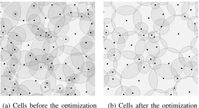
We introduce firstly an example of wireless network before and after the coverage optimization in Figure 8. In Figure 8a, the cells of the network are not optimized. Many cells overlap and the transmission power is wasted. In Figure 8b, the cells of the network are optimized. Some cells are turn off, the remaining cells work with optimized coverage radius. The overlapping region is minimized. As a result, it prevents the wasted transmission power. The transmission power of the network is reduced but the global coverage is kept unchanged. The performance of our distributed energy saving is eval-uated. It is also compared with the one obtained by the cen-tralized energy saving algorithm and the simulated annealing algorithm that are proposed in [7]. The simulated annealing
(a) Cells before the optimization (b) Cells after the optimization
Fig. 8: Cells before and after the optimization algorithm finds the global optimized solution. However, it has very big complexity and is not used in practice. The centralized one finds only a local minimum solution but it has smaller complexity.
We deploy the cells on a space[10 × 10] according to the Poisson point process. The density of cells is set to different values from 0.2 to 1. The coverage radius of each cell can vary from rmin = 0.1 to rmax = 1. We assume that the path
loss exponentγ is 3. The ˇCech complex with dimension two is enough to get the information about coverage and connectivity of the wireless network. So we do not need to build it up to a higher dimension as it causes longer computation time for the same information. Our simulations are repeated 1000 times.
1) Consumed power of optimized cells: Before the opti-mization, each cell is set to work with its maximum coverage radiusrmax= 1. At this state, each cell transmits the maximal
power, which is 1, following the Equation 2. After performing the energy saving algorithms, the average consumed power per cell with the optimized radius is shown in Figure 9.
0.2 0.4 0.6 0.8 1 0 0.1 0.2 0.3 0.4 0.5 0.6 0.7 0.8 Density of cells
Consumed power per cell
Simulated annealing algorithm Centralized energy saving algorithm Distributed energy saving algorithm
Fig. 9: Consumed power of optimized cells by different algorithms
The simulation shows that our distributed energy saving algorithm has better performance than the the centralized energy saving algorithm proposed in [7] at low density of cells. It also has the same performance with the centralized one at the high density of cells. The difference between the performance of our distribued energy saving algorithm with the one of the simulated annealing algorithm [7] is always less than 3%. However, our distributed energy saving algorithm has
much smaller complexity. At the highest density of cells, the cells optimized by the simulated annealing algorithm operate with 35% their original power, thus it saves 65% power. Our distributed algorithm saves 62% power.
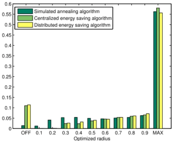
2) Probability density function of optimized cells’ radius:
We consider the pdf of the optimized radius of cells at different densities: high (1.0), medium (0.6), and low (0.2). They are presented in Figure 10, Figure 11, and Figure 12, respectively. While the pdf of cells radius optimized by our distributed energy saving algorithm and the centralized one [7] are quite similar, they are different from the one obtained by the simulated annealing algorithm [7]. The distributed and centralized energy saving algorithms turn off many cells. They turn off 35% and 10% of cells when the cells densities are high and low, respectively. The simulated annealing algorithm turns off less than 10% of cells at every density of cells.
OFF 0.1 0.2 0.3 0.4 0.5 0.6 0.7 0.8 0.9 MAX 0 0.05 0.1 0.15 0.2 0.25 0.3 0.35 0.4 0.45 Optimized radius
Probability density function
Simulated annealing algorithm Centralized energy saving algorithm Distributed energy saving algorithm
Fig. 10: Pdf of optimized radius at high density of cells (1.0)
OFF 0.1 0.2 0.3 0.4 0.5 0.6 0.7 0.8 0.9 MAX 0 0.05 0.1 0.15 0.2 0.25 0.3 0.35 0.4 0.45 Optimized radius
Probability density function
Simulated annealing algorithm Centralized energy saving algorithm Distributed energy saving algorithm
Fig. 11: Pdf of optimized radius at medium density of cells (0.6) OFF 0.1 0.2 0.3 0.4 0.5 0.6 0.7 0.8 0.9 MAX 0 0.05 0.1 0.15 0.2 0.25 0.3 0.35 0.4 0.45 0.5 0.55 0.6 Optimized radius
Probability density function
Simulated annealing algorithm Centralized energy saving algorithm Distributed energy saving algorithm
Fig. 12: Pdf of optimized radius at low density of cells (0.2)
The distributed and centralized algorithms avoid to keep active small cells while the simulated annealing one remains them. The advantage of the distributed energy saving algorithm is that it provides a similar performance as this simulated annealing one, while it requires a smaller number of active cells and has the smallest complexity.
The number of medium sized cells are quite similar at different densities of cells. There are 56% of cells work with the maximal coverage at low density of cells, but this number is only 22% at high density of cells. It means that the medium cells are substantial while the larger cells should be reduced in dense networks.
VI. CONCLUSION
This paper introduces the distributed computation of the ˇ
Cech complex aimed for self organized wireless networks. The complexity to compute the minimal ˇCech complex, which gives information about coverage and connectivity, is poly-nomial. A distributed application based on this distributed computation of the ˇCech complex is also proposed. This application aims at coverage optimization for energy saving in wireless networks. It has the same performance as the one of the centralized energy saving in [7] while having smaller complexity. The optimized network saves transmission power and only requires a small number of active cells, which allows to cut down the deployment costs.
Although homology theory gives information about cover-age and connectivity, it still locates and counts holes without measuring them. Its extension called persistent homology theory allows multi-scale analysis of the coverage of wireless networks. Applications of the ˇCech complex can be more developed with persistent homology theory.
REFERENCES
[1] Dimitris Bertsimas and John Tsitsiklis. Simulated annealing. Statist. Sci., 8(1):10–15, 02 1993.
[2] Stefan Dantchev and Ioannis Ivrissimtzis. Efficient construction of the ech complex. Computers & Graphics, 36(6):708 – 713, 2012. 2011 Joint Symposium on Computational Aesthetics (CAe), Non-Photorealistic Animation and Rendering (NPAR), and Sketch-Based Interfaces and Modeling (SBIM).
[3] Vin de Silva, Robert Ghrist, and Abubakr Muhammad. Blind swarms for coverage in 2-D. In Proceedings of Robotics: Science and Systems, Cambridge, USA, June 2005.
[4] H. Edelsbrunner and S. Parsa. On the computational complexity of betti numbers: Reductions from matrix rank. In Proceedings of the
Twenty-Fifth Annual ACM-SIAM Symposium on Discrete Algorithms, SODA ’14, pages 152–160. SIAM, 2014.
[5] Robert Ghrist and Abubakr Muhammad. Coverage and hole-detection in sensor networks via homology. In Proceedings of the 4th International
Symposium on Information Processing in Sensor Networks, IPSN ’05, Piscataway, NJ, USA, 2005. IEEE Press.
[6] Ngoc-Khuyen Le, P. Martins, L. Decreusefond, and A. Vergne. Con-struction of the generalized ˇCech complex. In Vehicular Technology
Conference (VTC Spring), 2015 IEEE 81st, pages 1–5, May 2015. [7] Ngoc-Khuyen Le, P. Martins, L. Decreusefond, and A. Vergne. Simplicial
homology based energy saving algorithms for wireless networks. In
Communication Workshop (ICCW), 2015 IEEE International Conference on, pages 166–172, June 2015.
[8] James Munkres. Elements of algebraic topology. Perseus Books, 1984. [9] Feng Yan, P. Martins, and L. Decreusefond. Connectivity-based
dis-tributed coverage hole detection in wireless sensor networks. In Global
Telecommunications Conference (GLOBECOM 2011), 2011 IEEE, pages 1–6, Dec 2011.