HAL Id: hal-03195185
https://hal.archives-ouvertes.fr/hal-03195185
Submitted on 10 Apr 2021
HAL is a multi-disciplinary open access
archive for the deposit and dissemination of
sci-entific research documents, whether they are
pub-lished or not. The documents may come from
teaching and research institutions in France or
abroad, or from public or private research centers.
L’archive ouverte pluridisciplinaire HAL, est
destinée au dépôt et à la diffusion de documents
scientifiques de niveau recherche, publiés ou non,
émanant des établissements d’enseignement et de
recherche français ou étrangers, des laboratoires
publics ou privés.
Mechanics of compliant serial manipulator composed of
dual-triangle segments
Wanda Zhao, Anatol Pashkevich, Damien Chablat, Alexandr Klimchik
To cite this version:
Wanda Zhao, Anatol Pashkevich, Damien Chablat, Alexandr Klimchik. Mechanics of compliant serial
manipulator composed of dual-triangle segments. International Journal of Mechanical Engineering
and Robotics Research, Dr. Bao Yang, 2021, 10 (4), pp.169-176. �10.18178/ijmerr.10.4.169-176�.
�hal-03195185�
Mechanics of compliant serial manipulator
composed of dual-triangle segments
Wanda Zhao, Anatol Pashkevich and Damien Chablat
Laboratoire des Sciences du Numérique de Nantes (LS2N), UMR CNRS 6004, Nantes, France Email: wanda.zhao@ls2n.fr, Anatol.Pashkevich@imt-atlantique.fr, Damien.Chablat@cnrs.fr
Alexandr Klimchik
Innopolis University, Tatarstan, Russia Email: A.Klimchik@innopolis.ru
Abstract—This paper focuses on the mechanics of a compliant serial manipulator composed of the new type of dual-triangle elastic segments. Both the analytical and numerical methods were used to find the stable and unstable equilibrium configurations of the manipulator, and to predict the corresponding manipulator shapes. The stiffness analysis was carried on for both loaded and unloaded modes, the stiffness matrices were computed using the Virtual Joint Method (VJM). The results demonstrate that either buckling or quasi-buckling phenomenon may occur under the loading if the manipulator initial configuration is straight or non-straight one. Relevant simulation results are presented at last, which confirm the theoretical study.
Index Terms—component, compliant manipulator, stiffness analysis, equilibrium, robot buckling, redundancy
I. INTRODUCTION
Currently, compliant serial manipulators are used more and more in many applications (such as inspection in constraint environment, medical fields etc.), because of their sophisticated motions and low weights. Conventional compliant manipulators are usually composed of rigid links and compliant actuators, like hinges, axles, or bearings. However, there is a lot of research in this area dealing with some new mechanical structures [1][2][3][4], which achieve compliant motions through tensegrity mechanisms. And one of them will be studied here.
In general, the robotic manipulators are usually classified into three types [5], conventional discrete, serpentine, and continuum robots. The first one is made of traditional rigid components. The second one uses discrete joints but combine very short rigid links with large density joints, which produce smooth curves and make the robot similar to a snake or elephant trunk [6]. While the continuum robots do not contain any rigid links or joints, they are very smooth and soft, bending continuously when working [7]. Many researchers have done studies on serpentine and continuum robots in recent years, designed flexible mechanisms for many
Manuscript received Sep, 2020; revised Sep 25, 2020; accepted Oct 9, 2020.
applications [8]. However, the pure soft continuum robot received little attention, as its small output force and design difficulty. Thus, combining rigid and elastic or soft components becomes a popular practice in designing a robot manipulator. The typical earlier hyper-redundant robot designs and implementations can be date back to the 1970s [9], which includes a series of plates interconnected by universal joints and elastic control components for pivotable action to one another. [10][11][12]
Nowadays, a very promising trend in designing compliant robots is using a series of similar segments based on various tensegrity mechanisms, which are composed in an equilibrium of compressive elements and tensile elements (cables or springs) [13][14]. Some kinds of tensegrity mechanisms have been already studied carefully. Such as [15], the authors dealt with the mechanism composed of two springs and two length-changeable bars. They analyzed the mechanism stiffness using the energy method, demonstrated that the mechanism stiffness always decreasing under external loading with the actuators locked, which may lead to “buckling”. And in [16][17], the cable-driven X-shape tensegrity structures were considered, the authors investigated the influence of cable lengths on the mechanism equilibrium configurations, which may be both stable and unstable. The relevant analysis of the equilibrium configurations stability and singularity can be seen in [18].
A new type of compliant tensegrity mechanism was proposed in our previous papers [19][20]. It is composed of two rigid triangle parts, which are connected by a passive joint in the center and two elastic edges on each side with controllable preload. The stiffness analysis of a basic dual-triangle was carried on, and the stable condition of the equilibrium was obtained. The results also showed that there may be a buckling phenomenon. Usually, while designing a robot, researchers always try to avoid buckling, but such behavior can make improvements in some fields [21]. So this phenomenon must be taken into account. In this paper, we study a compliant serial manipulator composed of the dual-triangle segments mentioned above, concentrate on the
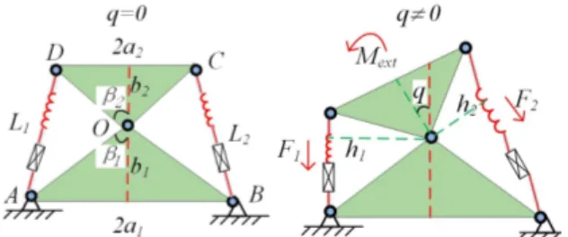
Figure 1. Geometry of a single dual-triangle mechanism.
equilibrium configurations and their transformations under the loading, which may be either continuous or sporadic that leading to buckling phenomenon. Both loaded and unloaded stiffness model of this manipulator were analyzed. The simulation of the manipulator behavior after buckling was obtained, which provides a good base of the design and relevant control algorisms of such manipulator
II. MECHANICS OF DUAL-TRIANGLE MECHANISM
Let us consider first a single segment of the compliant serial manipulator. It consists of two rigid triangles connected by a passive joint whose rotation is constrained by two linear springs as shown in Fig. 1. It is assumed that the mechanism geometry is described by the triangle parameters (a1, b1) and (a2, b2), and the mechanism shape
is defined by the central angle, which is adjusted through two control inputs influencing on the springs L1 and L2.
Let us denote the spring lengths in the non-stress state as
0 1
L and 0 2
L ,and the spring stiffness coefficients k1 and k2.
To find the mechanism configuration angle q corresponding to the given control inputs 0
1
L and 0 2
L , let us derive first the static equilibrium equation. From Hook’s law, the forces generated by the springs
are ( 0)
i i i i
F k L L (i =1, 2), where L1 and L2 are the
spring lengths |AD|, |BC|. These values can be computed
using the formulas 2 2
1 2 1 2 ( ) 2 cos( ) i i i L c c c c (i=1, 2). Here 2 2 i i i
c a b (i=1, 2), and the angles 1,2 are
expressed via the mechanism parameters as 112 , q 2 12 q
, and 12atan( / ) + atan( / )a b1 1 a b2 2 . The
torques M1=F1·h1, M1=F2·h2 in the passive joint O can be
computed from the geometry, so we can get
0 1 1 1 1 1 1 2 1 0 2 2 2 2 2 1 2 2 ( ) (1 ( )) sin( ) ( ) (1 ( )) sin( ) M q k L L c c M q k L L c c
where the difference in signs is caused by the different direction of the torques generated by the forces F1, F2.
Further, taking into account the external torque Mext
applied to the moving platform, the static equilibrium equation for the considered mechanism can be written as M1(q)+ M2(q)+Mext =0.
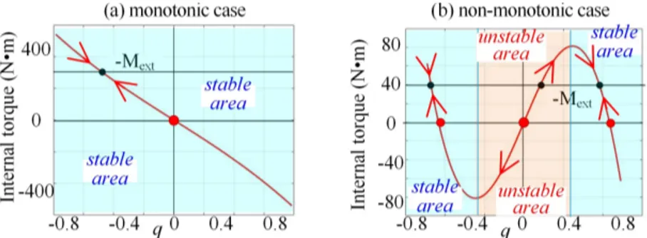
Let us now evaluate the stability of the mechanism under consideration. In general, this property highly depends on the equilibrium configuration defined by the angle q, which satisfies the equilibrium equation M(q)+
Mext =0. As follows from the relevant analysis, the
function M(q) can be either monotonic or non-monotonic one, so the single-segment mechanism may have multiple stable and unstable equilibriums, which are studied in detail [19][20]. As Fig. 2 shows, the torque-angle curves M(q) that can be either monotonic or two-model one, the considered stability condition can be simplified and reduced to the derivative sign verification at the zero point, i.e.
q 0 0M q (2)
which is easy to verify in practice. It represents the mechanism equivalent rotational stiffness for unloaded configuration with q=0.
Let us also consider in detail the symmetrical case, for which a1=a2=a, b1=b2=b, k1=k2, L =0i L . Then as follows 0
from the mechanism geometry, to distinguish the monotonic and non-monotonic cases presented in Fig. 2, we can omit some indices and present the torque-angle relationship as well as the stiffness expression in more compact forms:
0 12 1 0 12 1 2 22 cos sin cos( 2)s
2 cos cos cos c
in( 2) ( ) ( 2) o ( 2s ) M q ck c q L q M q ck c q L q (3)
it is also necessary to compute M’(q) for unloaded equilibrium configuration q=0, that let us obtain the condition of the torque-angle curve monotonicity:
0 2 1 ( )2
L b a b for the further analysis.
III. MECHANICS OF SERIAL MANIPULATOR
A. Manipulator Geometry and Kinematics
Let us consider a manipulator composed of three similar segments connected in series as shown in Fig. 3, where the left hand-side is fixed and the initial configuration is a “straight” one (q1=q2=q3=0). This
configuration is achieved by applying equal control inputs to all the mechanism segments. For this manipulator, it is necessary to investigate the influence of the external force Fe=(Fx, Fy), which causes the
end-effector displacements to a new equilibrium location
( , )T (6 , )T
x y
x y b , which corresponds to the
nonzero configuration variables (q1, q2, q3). It is also
assumed here the external torque Mext applied to the
end-effector is equal to zero. It can be easily proved from the geometry analysis that the configuration angles satisfy the following direct kinematic equations
1 12 123 1 12 123 2 2 2 2 x b bC bC bC y bS bS bS (4)
where C123cos
q1q2q3
, S123 sin
q1q2q3
,
12 cos 1 2
C q q , S12 sin
q1q2
, C1 cosq1 , 1 sin 1S q . These two equations include three unknown variables, and it allows us to compute two of them if the third one was known. For instance, if the angle q1 is
Figure 3. The torque-angle curves and static equilibriums for 0 0 1 2
L L (q0 ). 0 Figure 2. The torque-angle curves and static equilibriums for 0 0
1 2
L L (q0 ). 0
assumed to be known, the rest two angles q2, q3 can be computed from the classical inverse kinematics of the two-link manipulator as follows
3 3 3 3 1 2 1 1 3 atan 2 atan( ) atan( ) 2 2 q S C bS y bS q q x b bC b bC (5) where
2
2 2 2 3 2 1 2 1 5 4 C x b bC y bS b b , 2 3 1 3S C . The latter expressions provide two
groups of possible solutions, which correspond to the positive /negative configuration anglesq30andq30.
To find a stable manipulator configuration under the loading, let us apply the energy method. It is clear that the end-effector displacement caused by the external loading leads to the deflections of mechanism springs, which allows us to compute the manipulator energy as
3 2 2 0 1 1 1 2 ij ij i j E k L L
(6) where L andij o ijL are the spring lengths in current and initial (unextended) states respectively. The above energy can be expressed via one of the three variables q1, q2 or q3.
Assuming that variable q1 is chosen as an independent
one, the desired stable configurations can be found by computing local minima of the energy function
1
1
( ) min
q
E q (7)
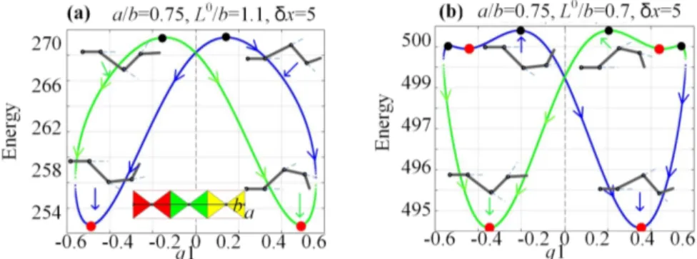
Examples of such energy curves E q( )1 for several typical
cases are presented in Fig. 4. B. Manipulator Stiffness Behavior
An alternative way to compute the configuration angles q1, q2, q3 at the equilibrium state is based on the
torque equation Me(q1)=0, which is implicitly used in the
energy method. The latter is illustrated by combined plots of the energy-torque curves computed for the initial “straight” configuration presented in Fig. 5, which shows that the max/min of the energy E(q1) correspond to zeros
of the torque Me(q1)=0. Further, to find the external
forces corresponding to this end-point location, it is necessary to use the force-torque equilibrium equation
0
M J FT
q
(8)
where M=(Mq1, Mq2, Mq3)T, F=(Fx, Fy, Me)T. They denote
the internal torques Mq1, Mq2 and Mq3 in all manipulator
segments and the force/torque at the end-point. In this equation, the internal torques can be computed using the previously derived expression from section II,
2 2 0
2 ( )sin sin(0.5 ) ; 1,2,3
qi i i
M k b a q bL q i (9)
and the Jacobian matrix Jq can be computed using the
standard technique for the three-link manipulator presented as follows 1 12 123 12 123 123 1 12 123 12 123 123 2 2 2 2 2 2 1 1 1 q bS bS bS bS bS bS bC bC bC bC bC bC J (10)
where S and C with corresponding indices have the same meaning as in (4). Assuming that the Jacobian is non-singular (i.e. the loaded manipulator is already out of the straight configuration), the external force/torque can be expressed directly as T
q
F J M, where the transport inverse matrix -T
q
J can be computed analytically. Then we can get the following expression
1 12 1 12 1 12 1 12 1 2 2 3 23 3 2 23 3 1 2 2 q x y q e q M F C C C C F S S S S M bS bS bS bS bS bS M M (11) The latter allows us to rewrite the system of the equilibrium equation (4) in the following extended form
Figure 4. Energy curves E q for different combinations of manipulator geometric parameters a/b, L( )1 o/b: “blue curves”─ positive configuration with q3>0; “green curves” ─ negative configuration with q3<0;
● ─ stable equilibrium; ● ─ unstable equilibrium
Figure 5. Correspondence between the maxima/minima of the energy curves E q and zeros of the external torque( )1 M q . e( )1
1 12 123 1 12 123 3 1 23 3 2 2 23 q3 2 2 0 2 2 0 2 0 q q b bC bC bC x bS bS bS y S M S S M S S M (12) whose solution (q1, q2, q3) may correspond to either stableor unstable equilibriums of the manipulator configuration. Then, using expressions Fx (q1, q2, q3) and Fy (q1, q2, q3)
obtained from (11), one can get the external loading (Fx ,
Fy) corresponding to the end-effector position (x, y),
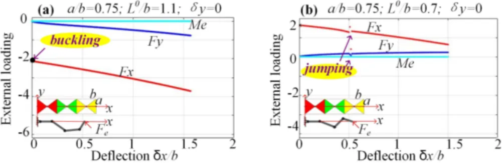
which finally allows us to generate the desired force-deflection curves. Examples of such curves for several case studies are presented in Fig. 6, where it is assumed that under the loading the manipulator moves along with x-axis, i.e.
xvar,
y0. As follows from this figure, in general cases (Fig. 6a), the force-deflection curves are quasi-linear, but some of them may do not pass through the zero point. The latter means that the corresponding manipulator possesses very specific particularity known as the “buckling” property [19][20][21], for which the configuration angles may suddenly change while the external force increasing gradually. Besides, in the case presented in Fig. 6b, there is the “jumping” phenomenon, because of the unstable geometrical parameters of the manipulator segment (see section II and stable condition ), and the manipulator suddenly changes its shape even for extremely small loading.To compute the critical force 0 x
F of the buckling, let us assume that the configuration angles (q1, q2, q3) are small
enough but not equal to zero. This allows us to derive a linearized stiffness model in the neighborhood of qi=0
(i=1, 2, 3). Under such assumptions, the first and second equations from (3.15) can be presented in the following form 2 2 2 1 12 123 1 12 123 ( 0.5 ) 2 ( 0.5 ) x y b q q q b q q q (13)
which allows us to present the condition δy=0 as q1+q12+
q123/2=0. Applying similar linearization to the third
equation from (12), one can get the additional relation of
the configuration angles 2 2
1 3 2 2 3 3 0
q q q q q q , which ensures the equality Me=0. Further, combining these two
obtained relations and considering q2 as an independent
variable, it is possible to express q1, q3 in the way
1 1 2
q
q , q3
3q2, where
1 21 11 20; 3 21 1 4
(14)
The latter gives us four possible manipulator geometric configurations corresponding to the static equilibrium, two with U-shape and two with Z-shape (see Table 1). The corresponding external forces Fx, Fy can be
linearized for small configuration angles, which yields
2 2 0 1 3 2 2 2( ) ( 2 ); 0 2 x y k F b a bL q q q F bq (15)
Further, taking into account (13) the desired critical force can be expressed in the following way
2 2 0 0 lim 2( ) i o x q x k F F b a bL b (16)
where ( 21 14) 10 0.9417 for U-shape, and
( 21 14) 10 1.8583
for Z-shape.
It is worth mentioning that the obtained expression allows us to derive the static stability condition for the straight configuration. In fact, this configuration is stable if and only if 0 0
x
TABLE I. POSSIBLE MANIPULATOR SHAPES IN STATIC EQUILIBRIUM
q1 q2 q3 Geometric configuration Stability
Case of “+√”
‒
+
+
U-shape: q1 q2 q3 Stable+
‒
‒
U-shape: q1 q2 q3 Stable Case of “-√”‒
+
‒
Z-shape: q1 q2 q3 Unstable+
‒
+
Z-shape: q1q2q 3 UnstableFigure 6. Force-deflection curves and stiffness coefficients for the “straight” initial configuration.
2 2
02 b a bL . It defining the monotonicity of the torque-angle curves for the manipulator segments.
Finally, let us compare the U-shape and Z-shape equilibrium configurations for their static stability. It can be easily proved that for the small configuration angles qi,
the end-effector deflection δx can be expressed in the
following way
2 2
x q
(17)where ( 21 21) 20 1.2791 for U-shape, and
( 21 21) 20 0.8209
for Z-shape. The latter
means that for the similar deflections δx, the U-shape has
the smaller configuration angles qi than the one of
Z-shape, which ensures smaller energy in agreement with (7).
Let us consider now when the manipulator initial configuration is non-straight, which corresponds to the angles (
q
i0
0,
i
1,2,3
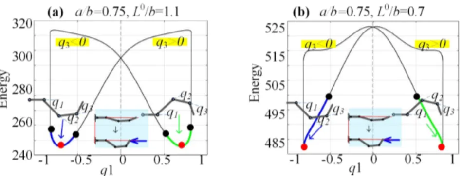
). Similar to the above section, the equilibrium is defined by three equations (12), which are derived from the direct kinematics and the zero external torque assumption Me=0. It can be proved thatthe energy curves have the “∞-shape” similar to the straight configuration considered before. However, depending on the initial end-effector location (x, y), these energy curves may be non-symmetrical and can be even discontinuous and include cusp points. Typical examples of such curves corresponding to the end-point location
T T
( , )
x y
(5.5 , 0)
b
are presented in Fig. 7, where the discontinuity caused by the geometric constraint is visible. In particular, the energy curve of cases (a) consists of two separate U-shape parts that yield two symmetrical stable equilibriums and four unstable ones. Such separation iscaused by the geometric constraints max i i
q q . However, the energy curves for the case (b) cannot be treated in the same way, because the combination of a, b, 0
i
L provides non-monotonic torque-angle curves for the segments and even separate parts of the manipulator are unstable here. It should be stressed that in the cases (a), each segment of the mechanism is statically stable. It should be also noted that there are some unfeasible sections (black lines) inside of the curve, where at least one of the angles q2 or
q3 is out of the allowable geometric limits.
The above-presented case studies, corresponding to the end-effector initial position
( , )
x y
T
(5.5 , 0)
b
T, can bealso illustrated by the force-deflection curves presented in Fig. 8. As follows, there is no buckling phenomenon in the case (a), the curve is quasi-linear and passes through the zero point. Besides, the buckling detected in the case (b) cannot be observed in practice because of the non-stability of the separate manipulator segments.
To evaluate the manipulator stiffness matrix for the non-straight configuration, let us first find the joint torques for all manipulator segments using the method from section II,
2 2 0 1 0 22 ( )sin( ) cos( 2) sin( 2)
cos( 2) sin( 2) ; 1,2,3 qi i i i i i i i M k b a q kL a q b q kL a q b q i (18) and compute the derivatives providing equivalent stiffness coefficients in the jointsKqidM dqqi i
2 2 0
1 0
2
2 ( )cos( ) cos( 2) sin( 2) 2
sin( 2) cos( 2 ) 2; 1, 2, 3 qi i i i i i i i i K k b a q kL b q a q kL a q b q i (19)
Figure 7. Energy curves E q for different (a, b, L( )1 o ) for non-straight initial configuration and displacement
x y,
b 2,0
“blue curves” ─ feasible configuration with q3>0; “green curves” ─ feasible configuration with q3<0;“black curves”─ unfeasible configuration; “red point ●”─ stable equilibrium; “black point ●” ─ unstable equilibrium..
Figure 8. Force-deflection curves and stiffness coefficients for “non-straight” initial configuration with different parameters (a, b, Lo ) and displacement
x y,
b 2,0
.This allows us to apply the VJM method and to express the unloaded stiffness matrix of the considered manipulator as
1 0 1 T F o qo o K J K J (20)where the subscript “o” denotes the variables corresponding to the unloaded initial configuration. Further, if we express the 2x3 submatrix of the (10) for this configuration as 11 12 13 21 22 23 2 3 o J J J J J J J (21)
The desired compliance matrix of the unloaded mode can be expressed analytically in the following way
2 2 2 13 11 12 0 1 1 2 3 2 2 2 23 21 22 1 2 3 * * T q q q F o qo o q q q J J J K K K J J J K K K C J K J (22)
where Kqodiag K( q1,Kq2,Kq3)is the matrix of size 3×3.
For the loaded mode, the manipulator stiffness matrix can be computed using the extended VJM technique proposed in [22]. Within this technique, let us assume that there is a non-negligible deflection ( x y, )T
caused by the external force ( , )T x y
F F
F , and there is a
small deflection ( x y, )T caused by this force
variation ( , )T
x y
F F
F that corresponds to the joint
angle variations T
1 2 3
( , , )
q q q q
. As follows fromthe equilibrium equation M J F= T , the corresponding
variation of the joint torque can be expressed as
T T d d J M q F J F q (23)
where the part dJT dq , which includes the Jacobian
derivative, can be rewritten as
3 T T 1 i g i i d q d q
J q F = J F K q q (24)where K is the 3×3 matrix describing the influence of g
loading F on the manipulator Jacobian J
1 2 3 3 3 T T T g q q q J J J K F F F (25)
that can be also written in the extended form as
21 11 22 12 23 13 22 12 22 12 23 13 23 13 23 13 23 13 3 3 x y x y x y g x y x y x y x y x y x y J F J F J F J F J F J F J F J F J F J F J F J F J F J F J F J F J F J F K (26)
Further, after expressing the virtual joint torque variation as M K qq and its substitution to (23), the variable
Figure 9. Force-deflection relations of three-segment mechanism for non-straight initial configuration with
x y, o 5.5 , 0b
.Figure 10. Evolution of the manipulator configuration under the loading.
1 Tq g
q K K J F (27)
which allows us to find the end-effector deflection
J q
, and finally to obtain the desired loaded compliance and stiffness matrices
1 T 1 1 T F q g F q g C J K K J K J K K J (28)It is worth mentioning that all the Jacobian and the joint stiffness matrices Kq, Kg must be computed for the
loaded equilibrium configuration, which is different from the initial unloaded one (It requires relevant solutions of the non-linear equations considered above).
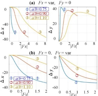
To illustrate the importance of the loaded stiffness analysis, the obtained expressions were applied to several cases study, which focusing on the manipulator stiffness changing under the external loading. For all considered cases, it was assumed that the initial manipulator configuration is a non-straight one, with the endpoint location (x0, y0)=(5.5b,0). Under the loading the
configuration angles corresponding to the external force F=(Fx, Fy)T were computed from (11) numerically (using
Newton’s Method). There are three combinations of the geometric parameters a/b ϵ{0.75; 0.9; 1.1}, relevant results are presented in Figs. 9 and 10. As follows from these figures, in most cases the manipulator stiffness essentially changes if the external loading is applied. In particular, the manipulator resistance in the x-direction becomes lower and lower while the force Fx is increasing
(see Fig. 9a). In contrast, the resistance in the y-direction with respect to the force Fy becomes higher and higher
while this force is increasing (see Fig. 9b). These results are also confirmed by the Kxx and Kyy plots presented in
Fig. 10, which show an enormous loss of x-direction resistance under the Fx loading (it can be treated as a
“quasi-buckling”, see Fig. 10a for the stiffness coefficient Kxx). On the other side, while increasing the force Fy, the
stiffness coefficient Kyy is very small at the beginning,
then it is increasing until reaches the maximum value, and then it is decreasing (see Fig. 10b). In this figure, an evolution of the manipulator configuration under the loading are also presented, with relevant stiffness coefficients Kxx and Kyy plots (corresponding to the case
a/b=0.75). They demonstrate the above mention results from the geometrical and physical point of view, which are corresponded to the stiffness coefficient and force relation. There are four representative configurations presented here, which showing the shapes of all segments and their position with respect to the joint limits. As follows from them, the observed sudden change of the stiffness (see Figs. 9 and 10) occurs if one of the segments is close to its joint limits, where the equivalent rotational stiffness coefficient is very low. Hence, in practice, it is necessary to avoid applying too high loading, or the manipulator will approach its joint limits and lose stiffness.
Therefore, as follows from the above study, the mechanical properties of a serial manipulator based on dual-triangle segments have several particularities, which are different from a classical serial structure composed of rigid links and compliant components. These particularities must be obligatory taken into account in control algorism, for ensuring desired motions of such manipulator, which is in the focus of our future research.
IV. CONCLUSION
The paper focuses on the compliant serial manipulator composed of a new type of dual-triangle tensegrity mechanism, which is composed of rigid triangles
connected by passive joints. In contrast to conventional cable-driven mechanisms, here there are two length-controllable elastic edges that can generate internal preloading. So, the mechanism can change its equilibrium configuration by adjusting the initial lengths of the elastic components.
The energy method was used to find the equilibrium configurations for different combinations of geometrical and mechanical parameters. The results show that both stable and unstable equilibriums may exist, and the manipulator shape will be an essential evolution if the external loading is applied. Some analytical results are presented, which allow us to find the manipulator shape under the loading and to estimate the stability of the corresponding configuration.
The manipulator stiffness analysis for both loaded and unloaded mode was done using the VJM method, and the relations between the end-effector deflection and the external force were obtained. Similar to the single dual-triangle segment, the buckling phenomenon occurs if the manipulator initial configuration is straight. Besides, for the non-straight initial configuration, the sudden change in deflection was also observed in some cases, which was treated as quasi-buckling. These particularities of the manipulator stiffness behavior were also observed in simulation.
The obtained results allowing to predict manipulator complicated behavior under the loading, and to avoid the buckling or quasi-buckling phenomenon by proper selection of the mechanical parameters, which will be used in the future for the development of relevant control algorisms and redundancy resolution.
ACKNOWLEDGMENT
This work was supported by the China Scholarship Council ( No. 201801810036 ).
REFERENCES
[1] M. I. Frecker, G. K. Ananthasuresh, S. Nishiwaki, N. Kikuchi, and S. Kota, “Topological Synthesis of Compliant Mechanisms Using Multi-Criteria Optimization,” Journal of Mechanical Design, vol. 119, no. 2, pp. 238–245, Jun. 1997, doi: 10.1115/1.2826242. [2] A. Albu-Schaffer et al., “Soft robotics,” IEEE Robotics
Automation Magazine, vol. 15, no. 3, pp. 20–30, Sep. 2008, doi: 10.1109/MRA.2008.927979.
[3] M. Y. Wang and S. Chen, “Compliant Mechanism Optimization: Analysis and Design with Intrinsic Characteristic Stiffness,” Mechanics Based Design of Structures and Machines, vol. 37, no. 2, pp. 183–200, May 2009, doi: 10.1080/15397730902761932. [4] L. L. Howell, “Compliant Mechanisms,” in 21st Century
Kinematics, London, 2013, pp. 189–216, doi: 10.1007/978-1-4471-4510-3_7.
[5] G. Robinson and J. B. C. Davies, “Continuum robots - a state of the art,” in Proceedings 1999 IEEE International Conference on Robotics and Automation (Cat. No.99CH36288C), May 1999, vol. 4, pp. 2849–2854 vol.4, doi: 10.1109/ROBOT.1999.774029. [6] G. S. Chirikjian and J. W. Burdick, “Kinematically optimal
hyper-redundant manipulator configurations,” IEEE Transactions on Robotics and Automation, vol. 11, no. 6, pp. 794–806, Dec. 1995, doi: 10.1109/70.478427.
[7] J. Yang, E. P. Pitarch, J. Potratz, S. Beck, and K. Abdel-Malek, “Synthesis and analysis of a flexible elephant trunk robot,”
Advanced Robotics, vol. 20, no. 6, pp. 631–659, Jan. 2006, doi: 10.1163/156855306777361631.
[8] G. S. Chirikjian and J. W. Burdick, “A modal approach to hyper-redundant manipulator kinematics,” IEEE Transactions on Robotics and Automation, vol. 10, no. 3, pp. 343–354, Jun. 1994, doi: 10.1109/70.294209.
[9] Anderson, Victor C., and Ronald C. Horn. "Tensor arm manipulator." U.S. Patent No. 3,497,083. 24 Feb. 1970.
[10] I. A. Gravagne and I. D. Walker, “Kinematic transformations for remotely-actuated planar continuum robots,” in Proceedings 2000 ICRA. Millennium Conference. IEEE International Conference on Robotics and Automation. Symposia Proceedings (Cat. No.00CH37065), Apr. 2000, vol. 1, pp. 19–26 vol.1, doi: 10.1109/ROBOT.2000.844034.
[11] R. Cieślak and A. Morecki, “Elephant trunk type elastic manipulator - a tool for bulk and liquid materials transportation,” Robotica, vol. 17, no. 1, pp. 11–16, Jan. 1999, doi: 10.1017/S0263574799001009.
[12] J. W. Hutchinson, “P o s t b u c k l i nTgheory,” p. 14.
[13] R. E. Skelton and M. C. de Oliveira, Tensegrity systems. Berlin: Springer, 2009.
[14] K. W. Moored, T. H. Kemp, N. E. Houle, and H. Bart-Smith, “Analytical predictions, optimization, and design of a tensegrity-based artificial pectoral fin,” International Journal of Solids and Structures, vol. 48, no. 22–23, pp. 3142–3159, Nov. 2011, doi: 10.1016/j.ijsolstr.2011.07.008.
[15] M. Arsenault and C. M. Gosselin, “Kinematic, static and dynamic analysis of a planar 2-DOF tensegrity mechanism,” Mechanism and Machine Theory, vol. 41, no. 9, pp. 1072–1089, Sep. 2006, doi: 10.1016/j.mechmachtheory.2005.10.014.
[16] M. Furet, M. Lettl, and P. Wenger, “Kinematic Analysis of Planar Tensegrity 2-X Manipulators,” in Advances in Robot Kinematics 2018, vol. 8, J. Lenarcic and V. Parenti-Castelli, Eds. Cham: Springer International Publishing, 2019, pp. 153–160.
[17] M. Furet, M. Lettl, and P. Wenger, “Kinematic Analysis of Planar Tensegrity 2-X Manipulators,” in Advances in Robot Kinematics 2018, vol. 8, J. Lenarcic and V. Parenti-Castelli, Eds. Cham: Springer International Publishing, 2019, pp. 153–160.
[18] P. Wenger and D. Chablat, “Kinetostatic analysis and solution classification of a class of planar tensegrity mechanisms,” Robotica, vol. 37, no. 7, pp. 1214–1224, Jul. 2019, doi: 10.1017/S026357471800070X.
[19] Zhao, W., Pashkevich, A., Klimchik, A. and Chablat, D., “Stiffness Analysis of a New Tensegrity Mechanism based on Planar Dual-triangles”. In Proceedings of the 17th International Conference on Informatics in Control, Automation and Robotics - Vol 1: ICINCO, July. 2020, ISBN 978-989-758-442-8, pages 402-411. doi: 10.5220/0009803104020411
[20] Zhao, W., Pashkevich, A., Klimchik, A. and Chablat, D., “The Stability and Stiffness Analysis of a Dual-Triangle Planar Rotation Mechanism”. In Proceedings of ASME 2020 International Design Engineering Technical Conferences And Computers and Information in Engineering Conference IDETC/CIE, Aug. 2020, (in press).
[21] A. Yamada, H. Mameda, H. Mochiyama, and H. Fujimoto, “A compact jumping robot utilizing snap-through buckling with bend and twist,” in 2010 IEEE/RSJ International Conference on Intelligent Robots and Systems, Taipei, Oct. 2010, pp. 389–394, doi: 10.1109/IROS.2010.5652928.
[22] S.-F. Chen and I. Kao, “Conservative Congruence Transformation for Joint and Cartesian Stiffness Matrices of Robotic Hands and Fingers,” The International Journal of Robotics Research, vol. 19, no. 9, pp. 835–847, Sep. 2000, doi: 10.1177/02783640022067201. Copyright © 2020 by the authors. This is an open access article distributed under the Creative Commons Attribution License (CC
BY-NC-ND 4.0), which permits use, distribution and reproduction in any
medium, provided that the article is properly cited, the use is non-commercial and no modifications or adaptations are made.