PROBABILISTIC 3D MODELING OF LAYERED SOIL DEPOSITS:
APPLICATION IN SEISMIC RISK ASSESSMENT
Mohammad Salsabili*, Ali Saeidi, Alain Rouleau
1Département des sciences appliquées, Université du Québec à Chicoutimi, Saguenay (Québec), Canada.
*Mohammad.salsabili1@uqac.ca ABSTRACT
Estimating the soil properties and the associated heterogeneity is critical in geotechnical risk assessment, particularly in a large urban area and for infrastructural development projects. Seismic hazard studies acknowledge the considerable impact of local soil conditions on the amplitude and frequency of incoming seismic waves. This is particularly challenging in areas with highly variable soil properties and limited soil sampling. A multi-step probabilistic approach is proposed to model the soil-types at a regional scale, involving a large database that incorporates surface and subsurface data with clustered sampling pattern, and highly skewed statistical parameter distributions. First, the Empirical Bayesian Kriging (EBK) method is applied for the interpolation of the total subsoil and till thickness. The results from the EBK method appear more accurate compared with the estimates from the triangulated irregular network. The soil-types and associated probability of occurrence are determined from the continuous till deposit at the bottom and the ground surface topography, using sequential indicator simulation. This simulation method allows predicting the probability of occurrence of discontinuous soil layers in the full 3D model, a real aspect of the soil variability. The predicted soil-types and their probabilities allow better consideration of key geological uncertainties in risk evaluation.
RÉSUMÉ
L’estimation des propriétés des sols et de leur hétérogénéité est essentielles pour l'évaluation des risques géotechniques, en particulier dans une grande zone urbaine et pour les projets de développement d’infrastructures. Les études sur les risques sismiques reconnaissent l'impact considérable des conditions locales du sol sur l'amplitude et la fréquence des ondes sismiques. Cela est particulièrement difficile dans les zones où les propriétés du sol sont très variables et où l'échantillonnage du sol est limité. Une approche probabiliste en plusieurs étapes est proposée pour modéliser les types de sols à l'échelle régionale, impliquant une grande base de données qui incorpore des données de surface et souterraines avec un modèle d'échantillonnage en grappes et des distributions statistiques très asymétriques des paramètres. La méthode de krigeage bayésien empirique (EBK) a été appliquée pour l'interpolation de l'épaisseur totale du sous-sol et du till. Les résultats de la méthode EBK sont plus exacts que les estimations obtenues par réseau triangulé irrégulier. Les types de sol et leur probabilité d’occurrence sont déterminés depuis le dépôt de till continu jusqu’à topographie de la surface du sol, à l'aide d'une simulation d'indicateur séquentiel. Cette méthode de simulation permet de prédire la probabilité d'occurrence de couches de sol non continues dans le modèle 3D complet, un aspect réel de la variabilité spatiale du sol. Les types de sols prévus et leurs probabilités permettent une meilleure prise en compte des facteurs géologiques clés dans l'évaluation probabiliste des risques géotechniques.
1 INTRODUCTION
Natural soils have heterogeneous properties due to differences in deposition geometry and process. Modeling soil heterogeneity should capture the soil properties and their spatial distribution adequately and allow assessing the associated uncertainties, including in the absence of site-specific or limited soil data. In geotechnics, soil heterogeneity is attributed to two main sources; one is rooted in the lithology and the other is the inherent spatial soil variability (Elkateb et al. 2003). The so-called lithological (soil-type) heterogeneity is related to the significant differences in the mineralogy,
grain size, and others, within a relatively uniform soil mass. This heterogeneity is described by qualitative terms (i.e., the soil-types), such as sand, clay, or stiff/soft soil layers. The second source of heterogeneity is rooted in inherent spatial soil variability, which modifies the spatial variation of soil properties due to different deposition conditions and different loading histories (Elkateb et al. 2003; Phoon et al. 2006). In the field of geotechnical engineering, the spatial variation of soil properties is modeled as a random field (Phoon and Kulhawy 1999; Uzielli et al. 2005) Recently, researchers have started using geostatistical approach to capture the heterogeneity in soil and rock engineering practices
(Ferrari et al. 2014; Kring and Chatterjee 2020; Vessia et al. 2020); this approach allows modeling the lithological heterogeneity.
In seismic hazard assessment, shear wave velocity and the thickness of soft soils play an important role in the amplification or de-amplification of seismic waves. In a regional study where data measured on shear-wave velocity (Vs) are sparse, the local geological
characteristics can be used as a proxy for estimating the shear wave velocity (Holzer et al. 2005; Thompson et al. 2014). Incorporating a 3D geological model to estimate the shear wave velocity were applied in several studies in eastern Canada (Rosset et al. 2015; Nastev et al. 2016; Foulon et al. 2018). These studies analyzed the uncertainty related to the geotechnical parameters and neglected the one related to the 3D geological model. Nevertheless, the type and the thickness of a soil layer, and the uncertainties associated with these parameters are essential parameters for the analysis of geotechnical risks.
This study aims to propose an innovative method of modeling the soil-types by considering the heterogeneities related to a model for a medium-to-large-scale region with data complexity. A combined multi-step approach of the interpolation and simulation method is adopted in order to address the data complexity of the observation points and to predict soil variability realistically. First, the soil-rock interface (total thickness of surficial soils) and the upper surface of the continuous till deposit are generated using the Empirical Bayesian Kriging (EBK) method. The interpolation procedure incorporates all boreholes data in addition to rock outcrops and thin-till data. Providing bedrock and till deposit maps help exclude a huge number of shallow and zero-thickness data from the simulation process of the discontinuous sediment layers (clay, sand, and gravel). The sequential indicator simulation is then used to predict the probability of occurrence of discontinuous soil layers as representing the real soil variability. 2 BACKGROUND
Empirical Bayesian Kriging (EBK) is a geostatistical
interpolation method that automates the process of fitting a variogram and solving a kriging model. This automated simulation process facilitates sub-setting data for large databases in regional studies. It potentially helps achieve stationarity in sub-areas, especially in a large dataset with a mixture distribution of high and low values. EBK is a novel interpolation method outperforming in the spatial prediction of data in large scale studies or data with complexities (Pilz and Spöck 2008; Krivoruchko and Gribov 2019; Giustini et al. 2019). The approach of locally varying mean and variance help assumption of the stationarity; the error variance provided by kriging can be the assessment of uncertainty about the estimated value.
Spatial variation denotes the dissimilarity (or
similarity) of a random variable between pairs of values as a function of their separation; it serves as important features of a spatial data set toward the estimation (Isaaks & Srivastava, 1989). An experimental variogram,
𝛾̂(ℎ), is used to statistically describe the average dissimilarity between data separated by a vector h (Goovaerts, 1999) and generally is a measure of spatial variability: 𝛾̂(ℎ) = 1 2 𝑁(ℎ)∑ [𝑧(𝑢𝛼) − 𝑧(𝑢𝛼+ ℎ)] 2 𝑁(ℎ) 𝛼=1 [1]
Where 𝑁(ℎ) is the number of data pairs within a distance h and direction. Key features of an experimental variogram are the range; the distance that the variogram reaches the plateau; the sill, the plateau that the variogram reaches. In addition to the nugget effect, the positive variogram value at extremely small separation distances which is attributed to the short scale variability (lower than the distance of sampling intervals) and measurement errors (e.g., errors in logging soil-types). With the delineation of the nugget effect, sill, and range, a theoretical model then fits the experimental variogram, which can be a spherical, exponential, or Gaussian model. Modeling spatial variation assists in predicting soil properties at unsampled locations.
Stochastic simulation of categorical variables such
as facies, rock types, or geological units is widely used in reservoir and mineral resource modeling (Deutsch 2006; Journel & Isaaks 1984; Pyrcz & Deutsch 2014). A stochastic modeling algorithm is applied to construct multiple realizations, and Sequential indicator simulation (SIS) is a widely used technique for categorical variable models (Deutsch 2006). A set of alternative, equally probable, high-resolution models of the spatial distribution of the random variable is constructed during the process; each realization reproduces the spatial statistics of the target variable (Deutsch & Journel, 1997). The method consists of three steps:
(i) Transferring soil types to K indicator variables:
𝑖(𝑢𝛼; 𝑘) = {1 𝑖𝑓 𝑐𝑎𝑡𝑒𝑔𝑜𝑟𝑦 𝑘 𝑝𝑟𝑒𝑣𝑎𝑖𝑙𝑠 𝑎𝑡 𝑙𝑜𝑐𝑎𝑡𝑖𝑜𝑛 𝑢
0 𝑜𝑡ℎ𝑒𝑟𝑤𝑖𝑠𝑒, 𝑘 = 1, … , 𝐾
Indicator transformation facilitates to carry out classical statistical analysis in order to infer representative proportions of indicator variables.
(ii) Defining indicator variograms to model the spatial continuity of indicator soil types. (iii) Simulating the soil types and honoring the
data values at their locations (conditional) in a sequential and reproducible procedure.
3 MATERIAL AND METHODS
3.1 Geologic Framework of the Study Area
The City of Saguenay is located in northeastern Quebec. It is the main municipality within the Saguenay‒Lac- Saint-Jean region and covers an area of 1136 km² with a population of 147,100. The city has a hilly topography and lies in the southern portion of the E–W-trending Saguenay graben. Regional seismic activity of this region was reassessed after the 1988 M6.0 Saguenay earthquake. The intraplate Saguenay earthquake, having a mid-crustal depth (29 km) and moderate
a b
Figure 1. (a) The simplified surface geological map of the Saguenay City territory (modified from Daigneault et al. 2011, CERM-PACES, 2013) (b) complete set of observation points including real and virtual boreholes, rock outcrops and thin
thickness till data magnitude, occurred 35 km south of the city center and
90 km to the northwest of the Charlevoix-Kamouraska seismically active zone (Du Berger et al. 1991).
Based on the geological sections (Daigneault et al. 2011) and subsurface data (CERM-PACES 2013), the various soil deposits can be split into two major groups glacial and post-glacial deposits (Walter et al. 2018). Glacial sediments located at the base of the stratigraphic column and continuously covers the bedrock. We consider this geologic rule as an important criterion in the 3D modelling approach.
The geologic terms at geological maps, sections, and borehole logs, can be grouped into five major groups based on the soil-types (Figure 1a):
1- Till, the glacial sediments located at the base of the stratigraphic column is compact, semi-consolidated, and is considered as continuous in the lowlands. The till ranges in thickness from a few meters to >10 m in locations. In the highlands, the till veneer is frequently discontinuous and results in areas of rock outcrops. The most area of the till outcrops is assigned less than 1 meter on the geological map (Daigneault et al. 2011).
2- Gravel, these coarse sediments are mainly attributed to the glaciofluvial deposits consisting gravel, sand and a little till. This unit is not widespread in the region and is limited to some contacts of till and sand units.
3- Clay, the most widespread and thickest deposits in the region are the fine postglacial sediments composed of silt, silty clays and clay. These silty clay deposits are generally up to 10 m in thickness, but they attain a thickness of >100 m in the lowlands.
4- Sand, this group consists mainly coarse glaciomarine deltaic and prodeltaic sediments composed of sand, and sandy gravel. Sandy alluvial sediments are also attributed to this group. 5- Others, loose postglacial deposits consisting of alluvium, floodplain sediments, organic sediments, and landslide deposits would classify to each three categories of sand, clay and gravel based on the logged soil types.
3.2 Data Preparation and Analysis
Subsurface and surfaced data were collected from various sources of information (Figure 1b). The drill hole logs are the main subsurface data from which the thickness data and soil-types are obtained. The other invaluable sources of data are rock outcrops with zero thickness value, virtual data derived from geological sections, and thin till data (thickness ≤ 1meter) interpreted from geological maps. The borehole data were obtained from groundwater wells, exploration boreholes, and geotechnical drilling logs. A complete set of data prepared for the study are:
Borehole logs: The borehole logs developed by PACES (CERM-PACES 2013) contain 3524 borehole logs distributes over the city of Saguenay territory. As a primary step, the thickness of 2402 boreholes, which known to reach the bedrock, determined and saved in the database. The thickness of 1122 boreholes not reaching the bedrock was used in the process of validation. Virtual boreholes: there are 26 geological
cross-sections over the region that are obtained by vast geological studies of PACES team. These sections have been interpreted from the stratigraphy observed in the boreholes and incorporated in previous studies (Chesnaux et al. 2017; Foulon et al. 2018). These cross-sections are distributed according to a regular spatial pattern to make a good coverage of the entire region. The number of 973 virtual boreholes are obtained alongside the cross-sections in a profile distance of 500 meters and consequently generate a regular pattern of drilling with reliable and validated information. Rock outcrops: these locations can be pointed out
as zero thickness data and can help enhance the realistic spatial variability. By spatial GIS processing of the geological map, 1034 rock outcrop points, located inside the bedrock polygon, were created to estimate the thickness of the total soil and till deposits.
Thin till data: till sediments covering the major area of this region are composed of zones with shallow
Figure 2. Histograms of the thickness of (a) total soil deposits (SGC) (b) total soil deposits and rock outcrops (SGC) (c) till sediments (d) till sediments after replacing outliers
thickness. The surface of thin till area was converted into a grid of points with a mesh of 75m. In this way, 42649 points with a thickness of 1meter were generated within the polygons of thin till area (Figure 2a). It should be noted this data is only applied to create the till thickness map.
Figure 2 shows the histograms of the thickness of total soil deposits and till deposits logged at the boreholes. The average thickness of soil materials are almost 17m with positive skewness, and the relatively high standard deviation of 18.7m illustrates the high variability of the thickness in the region. The maximum thickness of sediments reaches 112 m while the minimum reaches less than 1 meter in a close distance. Incorporation of rock outcrops with zero thickness data decreases the average of the thickness (12.89m), but the effects on the other parameters are minor (Figure 2b). Figure 2c illustrates the distribution of till thickness in boreholes. The average thickness of till is almost 5 in borehole logs, but it has been logged to almost 50m in maximum length. Because of the major influence of outliers on most parametric tests, considerable attention requires for the detection of outliers (Wu et al. 2011). Since the thickness of till rarely extends to more than 20 meters, the outlier data are the consequence of poor logging, replaced by the analysis of box-plot with a maximum of 13.85m (Figure 2d). Outliers were not replaced in the total thickness of soil deposits, as this would unrealistically decrease the estimated thickness of the deposits. Figure 3a illustrates the surface observation points, including thin till data (less than 1 m
in thickness) and rock outcrops (zero thickness data). These two sources of information improve the accuracy of the interpolation process while affecting the data distribution to the higher positive skewness and the lower mean of the thickness (Figure 3b).
3.3 Indicator Spatial Variation
To describe the spatial variability of categorical variables, firstly indicator transformation was performed, and then the indicator variograms were computed. The study analyzed the directional and omnidirectional variograms for the indicator soil-types using a lag size of 25m to model variability at a short scale, a lag size of 300m and 750m to capture variability at a long scale for gravel, and both sand and clay respectively. The bandwidth was chosen three times the lag size to restrict the deviation around the direction of the azimuth vector. Table 1 presents the variogram model parameters fitted to the soil-types indicators. The significant spatial variances were captured in short-scale variability, and the geometrical anisotropy with the azimuth angle of 135° corresponds to the geological continuity relatively (see Figure 1a). For all models, the vertical range is much less than the horizontal ranges; the anisotropy can be referred to as the large extension of soil type data in the horizontal direction relative to the vertical. Secondly, it would be due to the remarkable stratigraphic variation in the vertical direction than the horizontal.
Mean 17.73 Median 11.22 Standard Deviation 18.77 Kurtosis 2.76 Skewness 1.70 Minimum 0.01 Maximum 112.16 Count 2745 Mean 12.89 Median 5.79 Standard Deviation 17.84 Kurtosis 4.12 Skewness 2.00 Minimum 0.01 Maximum 112.16 Count 3778 Mean 5.74 Median 4.40 Standard Deviation 5.12 Kurtosis 13.75 Skewness 2.84 Minimum 0.00 Maximum 51.45 Count 1007 Mean 5.32 Median 4.40 Standard Deviation 3.67 Kurtosis 0.12 Skewness 0.97 Minimum 0.00 Maximum 13.85 Count 1007 a b c d
Figure 3. (a) surface observation points created from geological maps showing both the presence of thin till deposits in yellow (less than 1 m in thickness) and rock outcrops in red (zero thickness) (b) Histogram of the thickness of till sediments with all surface observation points.
Table 1- The variogram model parameters of the soil-type indicators
Variables N u mbe r o f s tr u c tu re s Model properties Structure 1 Model properties Structure 2 Model type Anisotropy axis
(amax,amed,amin) Model parameters
Model type
Anisotropy axis
(amax,amed,amin) Model parameters Clay 2 Sp. (135°,45°,90°) Nugget: 0.01 R1: (375,212.5,75) Sill1*: 0.18 Ex. (135°,45°,90°) R2: (12825,4275,75) Sill2*: 0.05 Sand 2 Sp. (135°,45°,90°) Nugget: 0.02 R1: (412.5,187.5,62.5) Sill1*: 0.17 Sp. (0°,0°,90°) R2: (12375,12375,62.5) Sill2*: 0.03 Gravel 2 Sp. - Nugget: 0.01 R1: (150,150,150) Sill1*: 0.026 Ga. (0°,0°,90°) R2: (4600,4600,150) Sill2*: 0.015 * Partial sill, R: Range, Sp.: Spherical, Ex.: Exponential, Ga.: Gaussian
4 RESULTS
4.1 Thickness Interpolation of Total Soil Deposits The study area was spatially discretized into a grid of 902 × 637 cells with 75-m spacing. Figure 4 illustrates the thickness map of the total soil deposits using (a) TIN, (b) EBK. The total thickness of the deposits varies from zero, represented by blue to approximately 100 meters represented by the reddish region.
4.2 Validation
There are 1122 boreholes are known not to reach the top of bedrock (see Figure 1b). These boreholes were reserved as a test set to evaluate the estimation methods. At these locations, if the model estimates the thickness less than the real value, it would be perceived that the depth of the observed point has been underestimated. Accordingly, an index of “thickness
error” considered by the difference between the measured and estimated thickness. The higher the number and the differences of the underestimations, the lower the precision of the estimation method.
Table 2 presents the descriptive statistical results of the thickness error containing the mean, the sum, and the
count of boreholes known not to reach the bedrock (validation dataset) according to the different interpolation methods. The EBK methods illustrated the least counts of underestimated boreholes by the number of 313. In contrast, the higher mean and the sum of the thickness error in the triangulated irregular network (TIN) method undermined the reliability of the estimates. Table 2. Descriptive statistical results of the thickness errors for the boreholes known not to reach the bedrock
Thickness error TIN EBK
Mean (m) 12.2 11.8
Sum (m) 3889.8 3682.6
Count 318 313
4.3 Thickness Interpolation of Till Deposits
The spatial distribution of the till thickness deposit was estimated using the EBK. The procedure is similar to the procedure of the total thickness interpolation in addition to the replacement of high peak values (outlier). The till deposits due to the difficulties in logging drilling muds are poorly recognized with the other soil types. Thus, Replacing outliers of the till thickness data would be
Mean 1.10 Median 1.00 Standard Deviation 0.86 Kurtosis 128.95 Skewness 10.70 Minimum 0.00 Maximum 13.85 Count 43656 a b
Figure 4. Thickness map of total soil thickness, (a) TIN, (b) EBK. considered as a conservative approach in the estimation of the thickness map. A complete set of observation points, including 2402 real and 973 virtual boreholes, 1034 rock outcrops as well as 42649 points of thin till thickness (1m) were incorporated to create the till thickness map. Figure 5 presents the spatial distribution of the till thickness and the associated kriging standard deviation. Replacing outliers and using thin till data avoided overestimating the till thickness, causing a conservative estimate for the future evaluation of the geotechnical soil parameters
Figure 5. Spatial distribution of the EBK estimates for the thickness till deposit
4.4 Soil-types Simulation
In order to determine the soil-types, a full 3D volume of blocks is required. Each block represents the smallest unit of soil-type using geostatistical simulation. For this purpose, it is necessary to create a bedrock topography and till topography using DEM, total thickness, and till thickness maps. When the bedrock topography, and the till topography were created, the space between the top and bottom of each surface was filled with blocks of 75×75×2 meters. The proportion of soil types was determined by using virtual boreholes due to the systematic and unclustered pattern. Overall, 100 realizations were generated using the sequential indicator simulation (SIS) method. Figure 6 shows the 3D spatial distribution of various soil types determined based on the most probability of occurrence. The results of the simulation were then compared to the geological
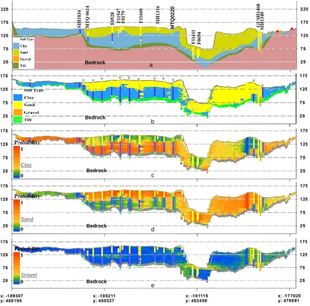
sections for visual validation. The results were found to be entirely consistent and acceptable (Figure 7). Figure 7a represents part of a main cross-section of the study area; the section interpreted and drawn by expert geologists using the surface geological map and subsurface data, mainly using borehole data in addition to some geophysical studies (CERM-PACES, 2013). Figure 7b shows the most probable soil-types blocks using SIS. The model used real and virtual borehole data. Due to the three-dimensional nature of the estimates, the model gave more realistic variability than the two-dimensional geological sections (Figure 7b, the area between borehole F1161 and SIH1340). Simulating soil types quantified the variability of the predictive model by the probability of occurrence (Figure 7 c-e) of three categorical variables, namely clay, sand, and gravel.
Figure 6. The 3D spatial distribution of various soil types using SIS based on the most probability of
occurrence 5 CONCLUSION
The study adopts a combined multi-step methodology of the interpolation and simulation methods to develop a 3D geological model for geotechnical risk evaluation at the regional scale. In a probabilistic geological model, the soil types are not deterministic and the quantified probabilities consider the spatial uncertainty of soil type. Consequently, these probabilities can be used to take into account the associated uncertainties in probability of failure in geotechnical risk assessment or site amplifications in seismic hazard assessment.
Figure 7. (a) a stratigraphic cross-section created by expert geologists (modified from CERM-PACES, 2013), (b) the most probable soil-types blocks using SIS, (c,d,e) probabilities of occurrence of each soil-types, obtained from a set of
100 conditional simulations This approach is based on the efforts to model the spatial
soil variability of both the continuous and the discontinuous soil layers. The depth to bedrock are distinguished by interpolating the total thickness of the sediments. The interpolation procedure incorporates the data from boreholes reaching the bedrock, in addition to rock outcrops and thin-till data, which cause an important skewness in observation points.
The results shows that the capability of the EBK method in sub setting data leads to a more accurate outcome in regional studies involving extensive data with complexity. Sequential indicator simulation predicts the probability of occurrence of discontinuous soil layers as representing the real spatial soil variability. The results reveal that the continuity assumption for the stratigraphic design of the clay, the sand and the gravel layers often drawn in the geological sections (CERM-PACES, 2013) would not correspond to the real variability of the soil deposits. This
is confirmed by abrupt discontinuities and repetitions of the deposits in the 3D model produced by using geostatistical simulation.
ACKNOWLEDGEMENT
The authors would like to thank the members of CERM-PACES project for providing access to the database and their fruitful cooperation. This research has been partially funded by the NSERC and Hydro-Quebec under project funding no. RDCPJ 521771 – 17.
REFERENCES
CERM-PACES, 2013. Résultat du Programme d’Acquisition de Connaissances sur les Eaux Souterraines de la Région Saguenay-Lac-Saint-Jean. Chicoutimi: Centre d’Études sur les Ressources Minérales, Université du Québec à Chicoutimi.
M T Q0 2 2 0 Bedrock Bedrock Bedrock Bedrock Bedrock Clay Sand Gravel a b c d e
Chesnaux, R., Lambert, M., Walter, J., Dugrain, V., Rouleau, A., & Daigneault, R. 2017. A simplified geographical information systems (GIS) -based methodology for modeling the topography of bedrock : illustration using the Canadian Shield. https://doi.org/10.1007/s12518-017-0183-1
Daigneault, R.-A., Cousineau, P., Leduc, E., Beaudoin, G., Millette, S., Horth, N., … G. Allard. 2011. Rapport final sur les travaux de cartographie des formations superficielles réalisés dans le territoire municipalisé du Saguenay-Lac-Saint-Jean. Quebec City: Ministère des
Ressources naturelles et de la Faune du Québec.
Deutsch, C. V. 2006. A sequential indicator simulation program for categorical variables with point and block data: BlockSIS. Computers and Geosciences, 32(10), 1669–1681.
https://doi.org/10.1016/j.cageo.2006.03.005
Deutsch, C. V, & Journel, A. G. 1997. GSLIB : Geostatistical Software Library and User ’ s Guide Second Edition Preface to the Second Edition. Du Berger, R., Roy, D. W., Lamontagne, M., Woussen, G.,
North, R. G., & Wetmiller, R. J. 1991. The Saguenay (Quebec) earthquake of November 25, 1988: seismologic data and geologic setting. Tectonophysics,
186(1–2), 59–74.
Elkateb, T., Chalaturnyk, R., & Robertson, P. K. 2003. An overview of soil heterogeneity : quantification and implications on geotechnical field problems, 15, 1–15. https://doi.org/10.1139/T02-090
Ferrari, F., Apuani, T., & Giani, G. P. 2014. Rock Mass Rating spatial estimation by geostatistical analysis.
International Journal of Rock Mechanics and Mining Sciences, 70, 162–176. https://doi.org/10.1016/j.ijrmms.2014.04.016
Foulon, T., Saeidi, A., Chesnaux, R., Nastev, M., & Rouleau, A. 2018. Spatial distribution of soil shear-wave velocity and the fundamental period of vibration– a case study of the Saguenay region, Canada. Georisk,
12(1), 74–86.
https://doi.org/10.1080/17499518.2017.1376253 Giustini, F., Ciotoli, G., Rinaldini, A., Ruggiero, L., &
Voltaggio, M. 2019. Mapping the geogenic radon potential and radon risk by using Empirical Bayesian Kriging regression: A case study from a volcanic area of central Italy. Science of the Total Environment, 661, 449–464.
https://doi.org/10.1016/j.scitotenv.2019.01.146 Goovaerts, P. 1999. Geostatistics in soil science :
state-of-the-art and perspectives, 1–45.
Holzer, T. L., Padovani, A. C., Bennett, M. J., Noce, T. E., & Tinsley, J. C. 2005. Mapping NEHRP VS30 site classes. Earthquake Spectra, 21(2), 353–370.
https://doi.org/10.1193/1.1895726
Isaaks, E. H., & Srivastava, M. R. 1989. Applied
geostatistics.
Journel, A. G., & Isaaks, E. H. 1984. Conditional indicator simulation: application to a Saskatchewan uranium deposit. Journal of the International Association for
Mathematical Geology, 16(7), 685–718.
Kring, K., & Chatterjee, S. 2020. Uncertainty quantification of structural and geotechnical parameter by geostatistical simulations applied to a stability analysis case study with limited exploration data. International
Journal of Rock Mechanics and Mining Sciences, 125(December 2018), 104157. https://doi.org/10.1016/j.ijrmms.2019.104157
Krivoruchko, K., & Gribov, A. 2019. Evaluation of empirical Bayesian kriging. Spatial Statistics, 32, 100368. https://doi.org/10.1016/j.spasta.2019.100368
Mirzaei, R., & Sakizadeh, M. 2016. Comparison of interpolation methods for the estimation of groundwater contamination in Andimeshk-Shush Plain, Southwest of Iran. Environmental Science and Pollution Research,
23(3), 2758–2769. https://doi.org/10.1007/s11356-015-5507-2
Nastev, M., Parent, M., Ross, M., Howlett, D., & Benoit, N. 2016. Geospatial modelling of shear-wave velocity and fundamental site period of Quaternary marine and glacial sediments in the Ottawa and St. Lawrence Valleys, Canada. Soil Dynamics and Earthquake
Engineering.
https://doi.org/10.1016/j.soildyn.2016.03.006
Phoon, K.-K., & Kulhawy, F. H. 1999. Characterization of geotechnical variability. Canadian Geotechnical Journal, 36(4), 612–624.
https://doi.org/10.1109/MED.2015.7158899
Pilz, J., & Spöck, G. 2008. Why do we need and how should we implement Bayesian kriging methods.
Stochastic Environmental Research and Risk Assessment, 22(5), 621–632. https://doi.org/10.1007/s00477-007-0165-7
Pyrcz, M. J., & Deutsch, C. V. 2014. Geostatistical
reservoir modeling. Oxford university press.
Rosset, P., Bour-Belvaux, M., & Chouinard, L. 2015. Microzonation models for Montreal with respect to VS30. Bulletin of Earthquake Engineering, 13(8), 2225–2239. https://doi.org/10.1007/s10518-014-9716-8
Uzielli, M., Vannucchi, G., & Phoon, K. K. 2005. Random field characterisation of stress-nomalised cone penetration testing parameters. Geotechnique, 55(1), 3–20.
Vessia, G., Di Curzio, D., & Castrignanò, A. 2020. Modeling 3D soil lithotypes variability through geostatistical data fusion of CPT parameters. Science of the Total
Environment, 698, 134340. https://doi.org/10.1016/j.scitotenv.2019.134340 Walter, J., Rouleau, A., Chesnaux, R., Lambert, M., &
Daigneault, R. 2018. Characterization of general and singular features of major aquifer systems in the Saguenay-Lac-Saint-Jean region. Canadian Water
Resources Journal, 43(2), 75–91.
https://doi.org/10.1080/07011784.2018.1433069 Wu, C., Wu, J., & Luo, Y. 2011. Spatial interpolation of
severely skewed data with several peak values by the approach integrating kriging and triangular irregular network interpolation, 1093–1103. https://doi.org/10.1007/s12665-010-0784-z