Deep generative models for fast shower simulation in
ATLAS
Kyle Cranmer Department of Physics
New York University [email protected] Stefan Gadatsch DPNC Université de Genève [email protected] Aishik Ghosh
LAL, Université Paris-Sud CNRS/IN2P3, Université Paris-Saclay
[email protected] Tobias Golling DPNC Université de Genève [email protected] Gilles Louppe Institut Montefiore Université de Liège [email protected] David Rousseau LAL, Université Paris-Sud CNRS/IN2P3, Université Paris-Saclay
[email protected] Dalila Salamani DPNC Université de Genève [email protected] Graeme Stewart CERN [email protected]
on behalf of the ATLAS Collaboration
Abstract
The need for large scale and high fidelity simulated samples for the extensive physics program of the ATLAS experiment at the Large Hadron Collider motivates the development of new simulation techniques. Building on the recent success of deep learning algorithms, Variational Auto-Encoders and Generative Adversarial Networks are investigated for modeling the response of the ATLAS electromag-netic calorimeter for photons in a central calorimeter region over a range of en-ergies. The properties of synthesized showers are compared to showers from a full detector simulation using Geant4. This feasibility study demonstrates the po-tential of using such algorithms for fast calorimeter simulation for the ATLAS experiment in the future and opens the possibility to complement current simula-tion techniques. To employ generative models for physics analyses, it is required to incorporate additional particle types and regions of the calorimeter and enhance the quality of the synthesised showers.
1
Introduction
The extensive physics program of the ATLAS experiment [1] at the Large Hadron Collider [2] relies on high-fidelity Monte Carlo (MC) simulation as a basis for hypothesis tests of the underlying distribution of the data. One of the key detector technologies used for characterizing collisions are calorimeters, measuring the energy and location of both charged and neutral particles traversing
the detector. Particles will lose their energy in a cascade (called a shower) of electromagnetic and hadronic interactions with a dense absorbing material. The number of the particles produced in these interactions is subsequently measured in thin sampling layers of an active medium.
The deposition of energy in the calorimeter due to a developing shower is a stochastic process that can not be described from first principles and rather relies on a precise simulation of the detector response. It requires the modeling of interactions of particles with matter at the microscopic level as implemented using the Geant4 toolkit [3]. This simulation process is inherently slow and thus presents a bottleneck in the ATLAS simulation pipeline [4].
To meet the growing analysis demands, ATLAS already relies strongly on fast calorimeter simula-tion techniques based on thousands of individual parametrizasimula-tions of the calorimeter response in the longitudinal and transverse direction given a single particle’s energy and pseudorapidity1 [5]. The algorithms currently employed for physics analyses by the ATLAS collaboration achieve a signif-icant speed-up over the full simulation of the detector response at the cost of accuracy. Current developments [6–8] aim at improving the modeling of tau leptons, jet-substructure-based boosted objects or wrongly identified objects in the calorimeter and will benefit from an improved detector description following data taking and a more detailed forward calorimeter geometry.
In recent years, deep learning algorithms have been demonstrated to accurately model the underlying distributions of rich, structured data for a wide range of problems, notably in the areas of computer vision, natural language processing and signal processing. The ability to embed complex distribu-tions in a low dimensional manifold has been leveraged to generate samples of higher dimensionality and approximate the underlying probability densities. Among the most promising approaches to gen-erative models are Variational Auto-Encoders (VAEs) [9, 10] and Gengen-erative Adversarial Networks (GANs) [11], shown to simulate the response of idealized calorimeters [12–14].
We present the first application of such models to the fast simulation of the calorimeter response of the ATLAS detector [15], demonstrating the feasibility of using such algorithms for large scale high energy physics experiments in the future, and open the possibility to complement current techniques. The presented studies focus on generating showers for photons over a range of energies in the central region of the electromagnetic calorimeter. Through the simplifications made, it is possible to focus on narrow regions of the calorimeter and neglect the dependence of the calorimeter response on the incident particle’s pseudorapidity.
2
ATLAS calorimeter
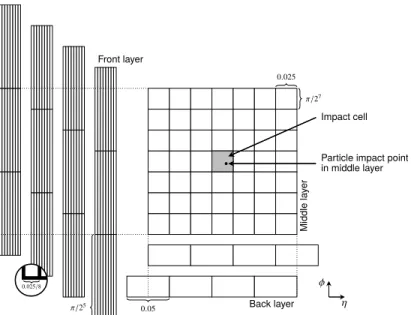
The ATLAS experiment at the LHC is a multipurpose particle detector with a forward-backward symmetric cylindrical geometry, covering nearly hermetically the full 4π solid angle by combining several sub-detector systems installed in layers around the interaction point. It comprises a calorime-ter system that is segmented into a matrix of three dimensional cuboids with varying shape and size, as illustrated in Fig. 1. Our work focuses on the electromagnetic (EM) calorimeter, providing en-ergy measurements for|η| < 2.5 with high granularity and longitudinal segmentation into multiple layers, capturing the shower development in depth. In the following, front, middle and back refer to the three layers in the central region of the EM barrel. In the region of|η| < 1.8, the ATLAS exper-iment is equipped with a presampler detector to correct for the energy lost by electrons and photons upstream of the calorimeter and thus to improve the energy measurements in these regions. The de-tailed structure of the calorimeter system influences the architecture of the deep studied generative models. Out of the EM barrel layers, the middle layer is the deepest and receives the maximum en-ergy deposit from EM showers. The front layer is thinner and exhibits a fine granularity in|η| < 1.4 (eight times finer than the middle layer), but four times less granular in ϕ. In the back layer less energy is deposited compared to the front and middle layers.
1
ATLAS uses a right-handed coordinate system with its origin at the nominal interaction point (IP) in the centre of the detector and the z-axis along the beam pipe. The x-axis points from the IP to the centre of the LHC ring, and the y-axis points upwards. Cylindrical coordinates (r, ϕ) are used in the transverse plane, ϕ being the azimuthal angle around the z-axis. The pseudorapidity is defined in terms of the polar angle θ as
0.025
π/27
0.05 π/25
Impact cell
Particle impact point in middle layer Middle la yer Back layer Front layer φ η 0.025/8
0.025
π/2
7
0.05
π/2
5
Impact cell
Particle impact point
in middle layer
Middle
la
yer
Back layer
Front layer
φ
η
0.025/8Figure 1: Illustration of possible alignments in ϕ for the front layer, (left, showing a 8× 3 portion of the 56× 3 cell image) and the back layer (bottom, showing a 4 × 1 portion of the 4 × 7 cell image) with respect to the middle layer (center, showing the full 7× 7 image). The front (back) layer are visualized to the left (bottom) of the middle layer to illustrate the alignments in ϕ (η), but are actually one behind another in the third dimension.
3
Monte Carlo samples and preprocessing
The ATLAS simulation infrastructure, consisting of event generation, detector simulation and dig-itization, is used to produce and validate the samples of single unconverted photons used for our studies. The samples are generated for nine discrete particle energies logarithmically spaced in the range between approximately 1 and 260 GeV and uniformly distributed in 0.20 <|η| < 0.25. Each simulated sample contains up to 10000 generated events, totaling approximately 90000 events avail-able for training and validation of the generative models. Alongside the energy deposited in the calorimeter cells, the detailed spatial position of each energy deposit is saved.
The showers originating from photons deposit almost their entire energy in the EM calorimeter and show little leakage into the hadronic calorimeter. Therefore only layers of the EM calorimeter are considered. Considering calorimeter cells as cuboids, for each layer the energy deposits within a rectangular selection are selected. The dimension of the rectangle for the middle layer is chosen to be 7× 7 cells in η × ϕ, with the cell hit by truth particle being in the center of the array. This selection contains more than 99 % of the total energy deposited by a typical shower in this layer. The dimensions of the remaining layers are chosen such that the spread in η and ϕ of the middle layer rectangle is covered. The dimensions for the presampler, front and back layer are 7× 3, 56 × 3 and 4× 7, respectively. All cells are selected with respect to the impact cell, defined as the cell in the middle layer closest to the extrapolated position of the photon, taking into account two possible alignments of the back layer and four possible alignments of the presampler and front layer with respect to the impact cell in the middle layer when considering the simplified cuboid geometry. This is illustrated in Fig. 1. In total the energy deposits in 266 cells are considered. For training the neural networks, the energy values are normalized to the energy of the incident particle.
4
Algorithms
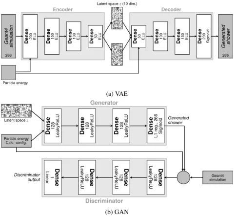
The explored VAE (Fig. 2a) is composed of two stacked neural networks, each comprising of 4 hidden layers, acting as encoder and decoder respectively. The number of units per layer decreases for subsequent layers of the encoder and increases for the decoder. The implemented algorithm is conditioned [16, 17] on the energy of the incident particle to generate showers corresponding to a specific energy. After training the model, the decoder can be used independently of the encoder
Encoder Decoder
Latent spacez(10 dim.)
Dense 50 ELU Dense 100 EL U Dense 150 EL U Dense 200 Sigmoid Gener at ed sho w er Dense 50 ELU Dense 100 EL U Dense 150 EL U Dense 200 EL U Geant4 simulation Particle energy 266 266 (a) VAE Generator Discriminator Dense 128 LeakyR eL U Dense 128 LeakyR eL U Dense 128 LeakyR eL U Dense L1 reg., 266 Sigmoid Particle energy Calo. config. Latent spacez Dense 1 Linear 128 Dense LeakyR eL U Dense 128 LeakyR eL U Dense 128 LeakyR eL U Geant4 simulation Generated shower Discriminator output (b) GAN
Figure 2: Schematic representation of the architecture of the studied (a) VAE and (b) GAN.
to generate new calorimeter showers by sampling from the prior probability density function of the latent space. The encoder and decoder networks are connected and trained together with mini-batch gradient descent using RMSProp [18]. The training maximizes the variational lower bound on the marginal log-likelihood for the data, approximated with reconstruction loss and the Kullback-Leibler divergence [19]. For fast calorimeter simulation, the objective function is further augmented with additional terms related to the total energy deposition of a particle and the fraction of the energy deposited in each calorimeter layer. The model is implemented in Keras 2.0.8 [20] using TensorFlow 1.3.0 [21] as the backend. The training of the VAE converges in 100 epochs within 2 min using the full available training statistics on a Intel⃝R CoreTM i7-7500U Processor with a
processor base frequency of 2.70 GHz and reading the training data from memory with a clock speed of 1867 MHz. Trainings for the hyperparameter optimization are performed in parallel on multiple CPUs. The last epoch of the training is used for synthesizing the presented showers. Originally developed for generating realistically looking natural images [11], GANs have a wide range of applications including calorimeter simulation [12–14]. The explored algorithm is com-posed of two neural networks, a generator and a discriminator (Fig. 2b). The model is conditioned on the energy of the incident particle and the alignments the calorimeter cells in η and ϕ. The generator and discriminator networks are trained together with mini-batch gradient descent using the Adam optimizer [22]. To introduce a measure of the distance between the true and synthesized showers and to increase the quality of the generated showers, the Wasserstein distance [23, 24] is used in the loss function [25, 26]. The Lipschitz constraint of the discriminator is enforced through employing a two-sided gradient penalty [25]. The model is implemented in Keras 2.0.8 [20] using TensorFlow 1.3.0 [21] as the backend. The training of the GAN, that is the discriminator and gen-erator networks, converges in 50000 epochs within 7 h using approximately 5 % of the available training statistics on a NVIDIA⃝R KeplerTMGK210 GPU with a processing power of 2496 cores,
each clocked at 562 MHz. The card has a video RAM size of 12 GB with a clock speed of 5 GHz. The training data is read from memory. Trainings for the hyperparameter optimization are performed in parallel on multiple GPUs. It is expected to increase the number of showers used for the training
while decreasing training times when fully utilising the distributed training capabilities and optimiz-ing the data processoptimiz-ing pipeline. The last epoch of the trainoptimiz-ing is used for synthesizoptimiz-ing the presented showers. Epoch-picking will be investigated in the future to cope with epoch-to-epoch fluctuations.
5
Results
For incident particles with varying energy, the models are trained to generate the corresponding calorimeter showers, i.e. the energy deposits in the 266 calorimeter cells considered in our setup. To assess the quality of the generation, the synthesized calorimeter showers are compared to the full detector simulation. Due to the stochastic nature of the shower development in the calorimeter, no individual shower can be compared. Instead, significant cumulative distributions used during the event reconstruction and particle identification, such as the total energy, the energy deposited in each calorimeter layer, and the relative distribution of energies in the calorimeter cells, are compared. These distributions typically correspond to projections of the data or moments computed from the magnitude and spatial position of the energy deposits. To quantify the agreement of the synthesized showers with the full detector simulation a χ2test is performed for each of these distributions.
As an example, Fig. 3 shows the total energy deposited in the middle layer of the calorimeter,
E2=
∑
j∈cells
E2j, (1)
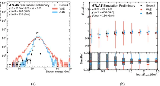
as well as their spatial distribution for photons with an energy of approximately 65 GeV in the range 0.20 <|η| < 0.25. Both VAE and GAN accurately describe the bulk of generated distributions, but the agreement in the tails of the distributions is reduced. The models reproduce the reference average lateral shower shape within a precision of approximately 20 to 40 % with differences increasing with the distance from the shower center.
The mean shower shape measured inside the calorimeter layers depends strongly on the longitudinal shower profile in the calorimeter and is used for example to distinguish photons from electrons. The modeling of the longitudinal shower development is shown for photons with an energy of approxi-mately 65 GeV in the range 0.20 <|η| < 0.25 in Fig. 3d. The reconstructed longitudinal shower center, in the following referred to as shower depth, is calculated from the energy weighted mean of the longitudinal center positions dlayerof all calorimeter layers,
d = 1 E
∑
i∈layers
Eidi. (2)
Both VAE and GAN reproduce the shape of shower depth simulated by Geant4, but the distribu-tions computed from the synthesized showers are shifted with respect to the Geant4 ones. This effect is explained by the mismodeling of the correlations between the energy deposits in the var-ious calorimeter layers and the challenges posed by layers with low (and sparse) energy deposits, i.e. showers starting not at the surface of the calorimeter.
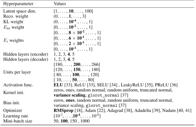
Figure 4a shows the total energy response of the calorimeter to photons with an energy of approxi-mately 65 GeV in the range 0.20 <|η| < 0.25,
E = ∑
i∈layers
∑
j∈cells
Eij. (3)
Figure 4b shows the simulated energy as a function of true photon energy. Both VAE and GAN reproduce the mean shower energy simulated by Geant4. The modeling of the total energy response reflects the modeling of the underlying distributions, i.e. the energy deposited in the calorimeter layers, and enhances the mismodeling of the tails due to underestimating the underlying correlations observed in these. Both generative models simulate a wider spread of energies than Geant4. The GAN reproduces better the correlations between the energy deposits in the different layers, and therefore shows a smaller spread than the VAE.
10 20 30 40 50 60 70 80 Energy [GeV] 101 102 103 104 Showers / 2 GeV
ATLAS Simulation Preliminary
γ, E = 65 GeV, 0.20 < |η| < 0.25 EM Barrel 2 χ2/ndf = 26 (VAE) χ2/ndf = 11 (GAN) Geant4 VAE GAN (a) -0.08 -0.06 -0.04 -0.02 0 0.02 0.04 0.06 0.08 Δη 10−1 100 101
Cell energy norm. to unity [GeV] / 0.025
ATLAS Simulation Preliminary
γ, E = 65 GeV, 0.20 < |η| < 0.25 EM Barrel 2 χ2/ndf = 50 (VAE) χ2/ndf = 270 (GAN) Geant4 VAE GAN (b) -0.08 -0.06 -0.04 -0.02 0 0.02 0.04 0.06 0.08 Δϕ [rad] 10−1 100 101
Cell energy norm. to unity [GeV] / 0.0245 rad
ATLAS Simulation Preliminary
γ, E = 65 GeV, 0.20 < |η| < 0.25 EM Barrel 2 χ2/ndf = 20 (VAE) χ2/ndf = 300 (GAN) Geant4 VAE GAN (c) 150 200 250 300 350
Shower depth with respect to presampler front [mm] 500 1000 1500 2000 2500 Showers / 10 mm
ATLAS Simulation Preliminary
γ, E = 65 GeV, 0.20 < |η| < 0.25 χ2/ndf = 16 (VAE) χ2/ndf = 26 (GAN) Geant4 VAE GAN (d)
Figure 3: (a) Energy deposited in the middle layer of the calorimeter as well as the average distribu-tion as a funcdistribu-tion of the distance in (b) η and (c) ϕ from the impact point of the particle and (d) the reconstructed longitudinal shower center for photons with an energy of approximately 65 GeV in the range 0.20 < |η| < 0.25. The chosen bin widths in (b) and (c) correspond to the cell widths in the calorimeter layer. The energy depositions from a full detector simulation (black markers) are shown as reference and compared to the ones of a VAE (solid red line) and a GAN (solid blue line). The shown error bars and the hatched bands indicate the statistical uncertainty of the reference data and the synthesized samples, respectively. The underflow and overflow is included in the first and last bin of each distribution, respectively.
40 50 60 70 80 90 Shower energy [GeV]
101 102 103 104 105 106 107 Showers / 1 GeV
ATLAS Simulation Preliminary
γ, E = 65 GeV, 0.20 < |η| < 0.25 χ2/ndf = 267 (VAE) χ2/ndf = 235 (GAN) Geant4 VAE GAN (a)
log10Etruth [GeV] 0.8 0.9 1 1.1 1.2 1.3 Esi m /Etr u th
ATLAS Simulation Preliminary
γ, 0.20 < |η| < 0.25 χ2/ndf = 400 (VAE) χ2/ndf = 130 (GAN) Geant4 VAE GAN 0 0.5 1 1.5 2 2.5
log10Etruth [GeV]
0.95 1.0 1.05
Sim./Ref.
(b)
Figure 4: (a) Total energy response of the calorimeter to photons with an energy of approximately 65 GeV in the range 0.20 < |η| < 0.25. The calorimeter response for the full detector simulation (black markers) is shown as reference and compared to the ones of a VAE (solid red line) and a GAN (solid blue line). The shown error bars and the hatched bands indicate the statistical uncertainty of the reference data and the synthesized samples, respectively. The underflow and overflow is included in the first and last bin of each distribution, respectively. (b) Energy response of the calorimeter as function of the true photon energy for particles in the range 0.20 < |η| < 0.25. The calorimeter response for the full detector simulation (black markers) is shown as reference and compared to the ones of a VAE (red markers) and a GAN (blue markers). The shown error bars indicate the resolution of the simulated energy deposits.
6
Conclusions
We present the first application of generative models for simulating particle showers in the ATLAS calorimeter. Two algorithms, a VAE and a GAN, have been used to learn the response of the EM calorimeter for photons with energies between approximately 1 and 260 GeV in the range 0.20 <
|η| < 0.25. The properties of synthesized showers show promising agreement with showers from
a full detector simulation using Geant4, demonstrating the feasibility of using such algorithms for fast calorimeter simulation for the ATLAS experiment in the future and opening the possibility to complement current techniques. In addition to conditioning the algorithms on different particle types and incorporating other regions of the calorimeter, further studies are needed to achieve the required accuracy for employing the algorithms for physics analyses.
A
ATLAS simulation infrastructure
The ATLAS simulation infrastructure, consisting of event generation, detector simulation and digitization, is used to produce and validate the samples used for the studies presented in this note. Samples of single unconverted photons are simulated using Geant4 10.1.patch03.atlas02, the standard MC16 RUN2 ATLAS geometry (ATLAS-R2-2016-01-00-01) with the conditions tag OFLCOND-MC16-SDR-14. The simulation employs the FTFP_BERT physics list [27], i.e. uses the Geant4 Bertini-style cascade [28–30] to simulate hadron-nucleus interactions at low incident hadron energies, and the Fritiof parton string model [31, 32] at higher energies, followed by the Geant4 precompound model to de-excite the nucleus. Specific to the version used by ATLAS is that the handover between the models is performed in the energy region between 9 GeV and 12 GeV.
B
Loss functions and domain knowledge
B.1 VAEThe evidence lower bound, i.e. the negative of the VAE loss, reads
log p(x)⩾ Eqθ(z|x)[log pϕ(x|z)] − KL(qθ(z|x)||p(z)), (4) where the Kullback-Leibler divergence, measuring the divergence between qθ(z|x) and the prior probability density function p(z), is defined as
KL(qθ(z|x)||p(z)) = n ∑ i=1
µ2i(xi) + σ2i(xi)− log(σi(xi))− 1 (5)
with µiand σientering qϕ(z/x) as the normal distributionN (z|µ, σ). For fast calorimeter simula-tion, the objective function is augmented with additional terms related to the total energy deposition of a particle, LEtot(x, ˜x) = k ∑ i=1 xi− k ∑ i=1 ˜ xi (6)
and the fraction of the energy deposited in each calorimeter layer,
LEi(x, ˜x) = ∑Ni j=1xj ∑k j=1xj − ∑Ni j=1x˜j ∑k j=1(˜xj) (7)
with the number of cells per shower shower, k, and the number of cells, Ni, in the i-th of M calorimeter layer. The full loss function then is
LVAE(x, ˜x) = wrecoEz∼qθ(z|x)[log pϕ(x|z)]−wKLKL(qθ(z|x)||p(z))+wEtotLEtot(x, ˜x)+
M ∑
i
wiLEi(x, ˜x). (8) Each term of the loss function is scaled by a weight, controlling the relative importance of the con-tributions during the optimization of the model. For example, the KL divergence acts as a regular-ization and changing its weight in the interval (0, 1] affects directly the generated distributions. The maximum value for the KL weight is 1, at which the loss becomes equivalent to the true variational lower bound, see Eq. 4.
B.2 GAN
The loss of the discriminator minimized in the training of the GAN reads
LGAN= E ˜ x∼pgen [D(˜x)]− E x∼pGeant4 [D(x)] + λ E ˆ x∼pxˆ [(||∆ˆxD(ˆx)||2− 1)2]. (9) The term E ˜ x∼pgen
[D(˜x)] represents the discriminator’s ability to correctly identify synthesized
show-ers, while the term E
x∼pGeant4
[D(x)] represents the discriminator’s ability to correctly identify showers from Geant4. The last term in the loss function, λ E
ˆ
x∼pxˆ
[(||∆xˆD(ˆx)||2−1)2], is the two-sided gradient
penalty, where ˆx is a random point on the straight line connecting a point from the real distribution pGeant4and generated distribution pgen.
C
Hyperparameter optimization
Tables 1 and 2 summarize the results of the grid search performed to optimize the hyperparameters of the VAE and GAN respectively. The parameters with the largest effect on the quality of the synthesized showers for the VAE are the weights considered for the various terms in the loss function and the dimension of the latent space. For the GAN the parameters with the largest effect on the quality of the synthesized showers are the choice of the activation functions and the conditioning.
Table 1: Summary the results of the grid search performed to optimize the hyperparameters of the VAE for simulating calorimeter showers for photons. The optimal parameter is typeset in bold font.
Hyperparameter Values
Latent space dim. [1, . . . , 10, . . . , 100] Reco. weight (0, . . . , 1, . . . , 3] KL weight (0, . . . , 10-4, . . . , 1] Etotweight [0, . . . , 10-2, . . . , 1] Eiweights [0, . . . , 8× 10⁻², . . . , 1] [0, . . . , 6× 10⁻¹, . . . , 1] [0, . . . , 2× 10⁻¹, . . . , 1] [0, . . . , 10-1, . . . , 1] Hidden layers (encoder) 1, 2, 3, 4, 5
Hidden layers (decoder) 1, 2, 3, 4, 5 Units per layer
[180, . . . , 200, . . . , 266] [120, . . . , 150, . . . , 180] [ 80, . . . , 100, . . . , 120] [ 10, . . . , 50, . . . , 80]
Activation func. ELU[33], ReLU [33], SELU [34] , LeakyReLU [35], PReLU [36] Kernel init. zeros, ones, random normal, random uniform, truncated normal,
variance scaling, glorot_normal [37]
Bias init. zeros, ones, random normal, random uniform, truncated normal, variance scaling, glorot_normal [37]
Optimizer RMSprop[18], Adam [22], Adagrad [38], Adadelta [39], Nadam [40, 41] Learning rate [10-2, . . . ,10-4, . . . , 10-6]
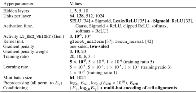
Table 2: Summary the results of the grid search performed to optimize the hyperparameters of the GAN for simulating calorimeter showers for photons. The optimal parameter is typeset in bold font. In addition to the architectures summarized in the table, generators and discriminators with differing number of hidden layers and units per layer were tested.
Hyperparameter Values
Hidden layers 1, 3, 5, 10
Units per layer 64, 128, 512, 1024 Activation func.
SELU [34] + Sigmoid, LeakyReLU [35] + {Sigmoid, ReLU [33], Gauss, Sigmoid + ReLU, clipped ReLU, softmax,
softmax + ReLU} Activity L1_REG_WEIGHT (Gen.) 0, 10-5, 10-2
Kernel init. glorot_uniform[37], lecun_normal [42] Gradient penalty one-sided, two-sided
Gradient penalty weight 0, 10, 20
Training ratio 20, 10, 5, 3, 1 Learning rate 5× 10⁻⁵, 5× 10⁻⁶, 1× 10⁻⁶(training ratio 5) 5× 10⁻⁵, 5× 10⁻⁶, 1× 10⁻⁵, 1× 10⁻⁷(training ratio 3) 1× 10⁻⁶(training ratio 1) Mini-batch size 64, 1024
Preprocessing (all norm. to Eγ) log10Ecell, log10(Ecell× 1010), Ecell
Conditioning {Eγ, log10Eγ} + multi-hot encoding of cell alignments
References
[1] The ATLAS Collaboration. The ATLAS Experiment at the CERN Large Hadron Collider.
JINST, 3:S08003, 2008. doi: 10.1088/1748-0221/3/08/S08003.
[2] Lyndon Evans and Philip Bryant. LHC Machine. JINST, 3:S08001, 2008. doi: 10.1088/ 1748-0221/3/08/S08001.
[3] S. Agostinelli et al. GEANT4: A Simulation toolkit. Nucl.Instrum.Meth., A506:250–303, 2003. doi: 10.1016/S0168-9002(03)01368-8.
[4] The ATLAS Collaboration. The ATLAS Simulation Infrastructure. Eur. Phys. J. C, 70:823, 2010. doi: 10.1140/epjc/s10052-010-1429-9.
[5] The ATLAS Collaboration. The simulation principle and performance of the ATLAS fast calorimeter simulation FastCaloSim. ATL-PHYS-PUB-2010-013, 2010. URL https://cds. cern.ch/record/1300517.
[6] Flavia Dias. The new ATLAS Fast Calorimeter Simulation. PoS, ICHEP2016:184, 2016. [7] Jana Schaarschmidt. The new ATLAS Fast Calorimeter Simulation. J. Phys. Conf. Ser., 898
(4):042006, 2017. doi: 10.1088/1742-6596/898/4/042006.
[8] The ATLAS Collaboration. The new Fast Calorimeter Simulation in ATLAS. ATL-SOFT-PUB-2018-002, 2018. URL https://cds.cern.ch/record/2630434.
[9] D. P Kingma and M. Welling. Auto-Encoding Variational Bayes. ArXiv e-prints, December 2013.
[10] D. Jimenez Rezende, S. Mohamed, and D. Wierstra. Stochastic Backpropagation and Approx-imate Inference in Deep Generative Models. ArXiv e-prints, January 2014.
[11] I. J. Goodfellow, J. Pouget-Abadie, M. Mirza, B. Xu, D. Warde-Farley, S. Ozair, A. Courville, and Y. Bengio. Generative Adversarial Networks. ArXiv e-prints, June 2014.
[12] Luke de Oliveira, Michela Paganini, and Benjamin Nachman. Learning Particle Physics by Example: Location-Aware Generative Adversarial Networks for Physics Synthesis. Comput.
[13] Michela Paganini, Luke de Oliveira, and Benjamin Nachman. Accelerating Science with Gen-erative Adversarial Networks: An Application to 3D Particle Showers in Multilayer Calorime-ters. Phys. Rev. Lett., 120(4):042003, 2018. doi: 10.1103/PhysRevLett.120.042003.
[14] Michela Paganini, Luke de Oliveira, and Benjamin Nachman. CaloGAN : Simulating 3D high energy particle showers in multilayer electromagnetic calorimeters with generative adversarial networks. Phys. Rev., D97(1):014021, 2018. doi: 10.1103/PhysRevD.97.014021.
[15] ATLAS Collaboration. Deep generative models for fast shower simulation in ATLAS. ATL-SOFT-PUB-2018-001, 2018. URL https://cds.cern.ch/record/2630433.
[16] Kihyuk Sohn, Honglak Lee, and Xinchen Yan. Learning structured output representation using deep conditional generative models. In C. Cortes, N. D. Lawrence, D. D. Lee, M. Sugiyama, and R. Garnett, editors, Advances in Neural Information Processing Systems 28, pages 3483–3491. Curran Associates, Inc., 2015. URL http://papers.nips.cc/paper/
5775-learning-structured-output-representation-using-deep-conditional-generative-models. pdf.
[17] J. Walker, C. Doersch, A. Gupta, and M. Hebert. An Uncertain Future: Forecasting from Static Images using Variational Autoencoders. ArXiv e-prints, June 2016.
[18] Tijmen Tieleman and Geoffrey Hinton. Lecture 6.5 – rmsprop: Divide the gradient by a run-ning average of its recent magnitude. Coursera: Neural networks for machine learrun-ning, 4(2): 26–31, 2012.
[19] S. Kullback and R. A. Leibler. On information and sufficiency. Ann. Math. Statist., 22(1): 79–86, 03 1951. doi: 10.1214/aoms/1177729694. URL https://doi.org/10.1214/aoms/ 1177729694.
[20] François Chollet et al. Keras, 2015. URL https://keras.io.
[21] Martín Abadi, Ashish Agarwal, Paul Barham, Eugene Brevdo, Zhifeng Chen, Craig Citro, Greg S. Corrado, Andy Davis, Jeffrey Dean, Matthieu Devin, Sanjay Ghemawat, Ian Goodfel-low, Andrew Harp, Geoffrey Irving, Michael Isard, Yangqing Jia, Rafal Jozefowicz, Lukasz Kaiser, Manjunath Kudlur, Josh Levenberg, Dandelion Mané, Rajat Monga, Sherry Moore, Derek Murray, Chris Olah, Mike Schuster, Jonathon Shlens, Benoit Steiner, Ilya Sutskever, Kunal Talwar, Paul Tucker, Vincent Vanhoucke, Vijay Vasudevan, Fernanda Viégas, Oriol Vinyals, Pete Warden, Martin Wattenberg, Martin Wicke, Yuan Yu, and Xiaoqiang Zheng. TensorFlow: Large-scale machine learning on heterogeneous systems, 2015. URL https: //www.tensorflow.org/.
[22] D. P. Kingma and J. Ba. Adam: A Method for Stochastic Optimization. ArXiv e-prints, De-cember 2014.
[23] Frank L. Hitchcock. The distribution of a product from several sources to numerous localities.
Journal of Mathematics and Physics, 20(1-4):224–230, 1941. doi: 10.1002/sapm1941201224.
[24] L.N. Vaserstein. Markovian processes on countable space product describing large systems of automata. Probl. Peredachi Inf., 5(3):64–72, 1969. ISSN 0555-2923.
[25] Ishaan Gulrajani, Faruk Ahmed, Martín Arjovsky, Vincent Dumoulin, and Aaron C. Courville. Improved training of wasserstein gans. 2017.
[26] M. Arjovsky, S. Chintala, and L. Bottou. Wasserstein GAN. ArXiv e-prints, January 2017. [27] J. Allison et al. Recent developments in Geant4. Nucl. Instrum. Meth., A835:186–225, 2016.
doi: 10.1016/j.nima.2016.06.125.
[28] M. P. Guthrie, R. G. Alsmiller, and H. W. Bertini. Calculation of the capture of negative pions in light elements and comparison with experiments pertaining to cancer radiotherapy. Nucl.
Instrum. Meth., 66:29–36, 1968. doi: 10.1016/0029-554X(68)90054-2.
[29] H. W. Bertini. Intranuclear-cascade calculation of the secondary nucleon spectra from nucleon-nucleus interactions in the energy range 340 to 2900 mev and comparisons with experiment.
[30] H. W. Bertini and M. P. Guthrie. News item results from medium-energy intranuclear-cascade calculation. Nucl. Phys., A169:670–672, 1971. doi: 10.1016/0375-9474(71)90710-X. [31] Bo Andersson, G. Gustafson, and B. Nilsson-Almqvist. A Model for Low p(t) Hadronic
Reac-tions, with Generalizations to Hadron - Nucleus and Nucleus-Nucleus Collisions. Nucl. Phys., B281:289–309, 1987. doi: 10.1016/0550-3213(87)90257-4.
[32] Bo Nilsson-Almqvist and Evert Stenlund. Interactions Between Hadrons and Nuclei: The Lund Monte Carlo, Fritiof Version 1.6. Comput. Phys. Commun., 43:387, 1987. doi: 10.1016/ 0010-4655(87)90056-7.
[33] Djork-Arné Clevert, Thomas Unterthiner, and Sepp Hochreiter. Fast and accurate deep network learning by exponential linear units (elus). 2015.
[34] Günter Klambauer, Thomas Unterthiner, Andreas Mayr, and Sepp Hochreiter. Self-normalizing neural networks. 2017.
[35] Andrew L. Maas, Awni Y. Hannun, and Andrew Y. Ng. Rectifier nonlinearities improve neural network acoustic models. In in ICML Workshop on Deep Learning for Audio, Speech and
Language Processing, 2013.
[36] Kaiming He, Xiangyu Zhang, Shaoqing Ren, and Jian Sun. Delving deep into rectifiers: Sur-passing human-level performance on imagenet classification. 2015.
[37] Xavier Glorot and Yoshua Bengio. Understanding the difficulty of training deep feedforward neural networks. In Yee Whye Teh and Mike Titterington, editors, Proceedings of the
Thir-teenth International Conference on Artificial Intelligence and Statistics, volume 9 of Proceed-ings of Machine Learning Research, pages 249–256, Chia Laguna Resort, Sardinia, Italy, 13–
15 May 2010. PMLR. URL http://proceedings.mlr.press/v9/glorot10a.html. [38] John Duchi, Elad Hazan, and Yoram Singer. Adaptive subgradient methods for online learning
and stochastic optimization. J. Mach. Learn. Res., 12:2121–2159, July 2011. ISSN 1532-4435. URL http://dl.acm.org/citation.cfm?id=1953048.2021068.
[39] Matthew D. Zeiler. ADADELTA: an adaptive learning rate method. 2012.
[40] Ilya Sutskever, James Martens, George Dahl, and Geoffrey Hinton. On the importance of initialization and momentum in deep learning. In Sanjoy Dasgupta and David McAllester, editors, Proceedings of the 30th International Conference on Machine Learning, volume 28 of
Proceedings of Machine Learning Research, pages 1139–1147, Atlanta, Georgia, USA, 17–19
Jun 2013. PMLR. URL http://proceedings.mlr.press/v28/sutskever13.html. [41] Timothy Dozat. Incorporating nesterov momentum into adam. 2015.
[42] Yann LeCun, Leon Bottou, Genevieve B. Orr, and Klaus-Robert Müller. Efficient BackProp, pages 9–50. Springer, 1998. ISBN 978-3-540-49430-0. doi: 10.1007/3-540-49430-8_2. URL https://doi.org/10.1007/3-540-49430-8_2.