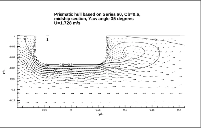
Preliminary estimates of flow patterns around hulls with yaw angle

In the following we briefly compare the transition scenario with another bluff body wake : the cube wake. Transitions of the cube wake have been studied by Saha [50]. Both cylinder

However, the laboratory experiment revealed that for the wave amplitude used, the reflected wave and the second harmonic wave are considerably weaker compared to the incident wave,

Eventually, we apply our result to the positive curvature flow in two dimensions, obtaining a short time existence and uniqueness result (Corollary 6.5) for C 1,1 -regular

The opposite might also be true: simple shaped monotonically decreasing dye coverage functions are usually the result of homogenous flow processes (not necessarily uniform

To end the proof and in particular to remove the flat remainder term O Σ (∞) in the Birkhoff normal form given in Theorem 2.2, we use the nice scattering method due to Edward

While MultiInstance pattern introduced in the previous paragraph implements the ability to create more instances from one node, this pattern focuses on the data aspects of this

We highlight a pronounced quasi 2 year peak in the anomalous zonal wind and eddy momentum flux convergence power spectra in the Southern Hemisphere, which is prima facie evidence

As the paper focuses on the transitions between the different flow patterns, the strategy employed is to keep a constant mean flow (water depth and mean