Annular modes and apparent eddy
feedbacks in the Southern Hemisphere
The MIT Faculty has made this article openly available.
Please share
how this access benefits you. Your story matters.
Citation
Byrne, Nicholas J. et al. “Annular Modes and Apparent Eddy
Feedbacks in the Southern Hemisphere.” Geophysical Research
Letters 43.8 (2016): 3897–3902.
As Published
http://dx.doi.org/10.1002/2016GL068851
Publisher
American Geophysical Union (AGU)
Version
Final published version
Citable link
http://hdl.handle.net/1721.1/106332
Terms of Use
Creative Commons Attribution-NonCommercial-NoDerivs License
Annular modes and apparent eddy feedbacks
in the Southern Hemisphere
Nicholas J. Byrne1, Theodore G. Shepherd1, Tim Woollings2, and R. Alan Plumb3
1Department of Meteorology, University of Reading, Reading, UK,2Department of Physics, Atmospheric, Oceanic and
Planetary Physics, Oxford, UK,3Department of Earth, Atmospheric and Planetary Sciences, Massachusetts Institute of
Technology, Cambridge, Massachusetts, USA
Abstract
Lagged correlation analysis is often used to infer intraseasonal dynamical effects but is known to be affected by nonstationarity. We highlight a pronounced quasi 2 year peak in the anomalous zonal wind and eddy momentum flux convergence power spectra in the Southern Hemisphere, which is prima facie evidence for nonstationarity. We then investigate the consequences of this nonstationarity for the Southern Annular Mode and for eddy momentum flux convergence. We argue that positive lagged correlations previously attributed to the existence of an eddy feedback are more plausibly attributed to nonstationary interannual variability external to any potential feedback process in the midlatitude troposphere. The findings have implications for the diagnosis of feedbacks in both models and reanalysis data as well as for understanding the mechanisms underlying variations in the zonal wind.1. Introduction
Fluctuations in the strength and location of the zonally averaged westerlies have long been recognized as an important pattern of atmospheric low-frequency variability. Such fluctuations are also seen across a wide hierarchy of numerical models.
The study of these variations is frequently investigated with the use of empirical orthogonal function (EOF) analysis. This has the effect of significantly reducing the dimensionality of the data to be analyzed while arguably preserving the underlying physical mechanisms. In the Southern Hemisphere the leading EOF of the zonal wind anomalies is referred to as the Southern Annular Mode (SAM). It is the dominant pattern of climate variability affecting the Southern Hemisphere extratropics, is present in every season, and is interpreted as a poleward/equatorward shift of the westerlies [Hartmann and Lo, 1998].
It is well established from physical principles that momentum flux convergence anomalies (hereafter referred to as “anomalous eddy flux convergence”) force the zonal wind anomalies. This can be seen by considering the zonally and vertically integrated quasi-geostrophic momentum equation:
dz dt = m −
z
𝜏, (1)
Here z represents an index for the zonal wind anomalies, m an index for the anomalous eddy flux convergence, and𝜏 a timescale approximating damping of the zonal wind anomalies by frictional processes.
As a result of the equivalent barotropic structure of the SAM, equation (1) is often used as a conceptual model for studying SAM dynamics. In this case z represents SAM variations and m represents an index for the anoma-lous eddy flux convergence projected onto the SAM. This approximation is found to hold well in reanalysis data [Lorenz and Hartmann, 2001].
In the presence of white noise forcing by m (anomalous eddy flux convergence) such a system is known to exhibit low-frequency variability in z (SAM) [e.g., Hasselmann, 1976]. For the true climate system it is of con-siderable interest whether the low-frequency variability in the SAM is also modified by the existence of a feedback process on the anomalous eddy flux convergence, behavior which has previously been shown to exist in idealized numerical models [e.g., Robinson, 1996]. Such a (positive) feedback could act to increase the persistence of the SAM and could thus account for much of the low-frequency variability in the extratropics.
RESEARCH LETTER
10.1002/2016GL068851
Key Points:
• Analysis of lagged correlations between Southern Annular Mode and eddy momentum flux convergence in reanalysis data
• Previous evidence for an eddy feedback more plausibly interpreted as nonstationary interannual variability
• Southern Annular Mode and eddy momentum flux convergence power spectra exhibit a pronounced quasi 2 year peak Correspondence to: N. J. Byrne, [email protected] Citation: Byrne, N. J., T. G. Shepherd, T. Woollings, and R. A. Plumb (2016), Annular modes and apparent eddy feedbacks in the South-ern Hemisphere, Geophys.
Res. Lett., 43, 3897–3902,
doi:10.1002/2016GL068851.
Received 11 DEC 2015 Accepted 5 APR 2016
Accepted article online 11 APR 2016 Published online 21 APR 2016
©2016. The Authors.
This is an open access article under the terms of the Creative Commons Attribution-NonCommercial-NoDerivs License, which permits use and distribution in any medium, provided the original work is properly cited, the use is non-commercial and no modifications or adaptations are made.
Geophysical Research Letters
10.1002/2016GL068851
An understanding of the relationship between the SAM and the anomalous eddy flux convergence is thus important for the problem of predicting the intraseasonal variability of the zonal wind in the extratropics. It is also of considerable importance for quantifying the long-term response to climate forcing [e.g., Ring and Plumb, 2007, 2008].
To diagnose potential feedback behavior, a framework has been developed using the method of lagged regression analysis [Hasselmann, 1976; Frankignoul and Hasselmann, 1977]. This framework requires that there be a clear timescale separation between the components of the system (in this case between the anomalous eddy flux convergence and the SAM) and assumes the feedback to be a linear process. Such a timescale sepa-ration between the anomalous eddy flux convergence and the SAM has been previously verified in reanalysis data [Lorenz and Hartmann, 2001].
In the lagged regression framework, for those lags where the anomalous eddy flux convergence leads the SAM, increasing correlation values have been found from about 20 days up to 2 days [e.g., Feldstein, 1998]. This is as expected theoretically for a system that obeys (1). More significantly, positive correlations at lags where the SAM leads the anomalous eddy flux convergence have also been documented, and these have been attributed to the presence of an eddy feedback mechanism [e.g., Lorenz and Hartmann, 2001]. This eddy feedback mechanism is now a well-accepted concept in the literature [e.g., Kushner, 2010].
Causal attribution in this lagged regression framework is subject to the additional assumption that the low-frequency portion of the power spectrum of the anomalous eddy flux convergence is white in the absence of a feedback [Frankignoul and Hasselmann, 1977], i.e., that the anomalous eddy flux convergence is not influ-enced by nonstationary interannual variability. This is a significant assumption as there is ample evidence of interannual variability in the midlatitude troposphere of both hemispheres that is externally forced, e.g., from the tropics or the stratosphere [L’Heureux and Thompson, 2006; Lu et al., 2008; Simpson et al., 2011; Anstey and Shepherd, 2014]. In light of this we revisit earlier results to see if they can be more naturally explained in terms of nonstationary interannual variability in the extratropics.
2. Data and Methods
We use four-times-daily wind data from the ERA-Interim reanalysis data set [Dee et al., 2011] for the period January 1980 to December 2013. Data were available on an N128 Gaussian grid and on 27 pressure levels (1000–100 hPa). The indices for the SAM and for the anomalous eddy flux convergence were computed using daily mean values as per Lorenz and Hartmann [2001].
The cross correlation plots were estimated following Von Storch and Zwiers [2002] (see Appendix A). To assess significance of the cross-correlation values, a formula suggested by Bartlett [see Von Storch and Zwiers 2002, section 12.4.2 ] was used throughout (see Appendix B).
For the spectral analysis the year-round indices for the SAM and for the anomalous eddy flux convergence were first windowed by a Hanning window. The raw periodogram was then computed from this windowed data. Finally a smoothed estimate of the spectrum was calculated by successive application of modified Daniell filters of length 6, 12, and 12 to the raw periodogram following Bloomfield [2000].
3. Results
3.1. SAM and Anomalous Eddy Momentum Flux Convergence Power Spectra
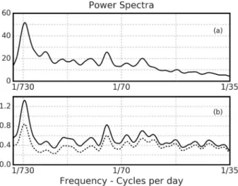
To investigate the hypothesis of externally forced influence on the SAM and the anomalous eddy flux conver-gence, power spectra from reanalysis data were computed (Figures 1 and 2). The power spectrum of the SAM is shown in Figures 1a and 2a. It offers evidence that there is considerable variability on interannual timescales with increasing power at lower frequencies. This increase of power at lower frequencies is in qualitative agreement with theoretical predictions from (1) [Hasselmann, 1976].
The SAM power spectrum also suggests that interannual variability might be organized in a very particular way as there is a distinct peak at a quasi 2 year period. This quasi 2 year peak is also present in the anomalous eddy flux convergence power spectrum (Figures 1b and 2b). In contrast to the inherent high-frequency variability of the eddies (Figure 1b), this low-frequency peak occurs on climate timescales.
To determine whether this peak is consistent with an eddy feedback or in fact represents nonstationary inter-annual variability, we consider here whether the spectral peak can be reproduced by assuming a linear model
Figure 1. Power spectral density plots for (a)z(SAM) and (b)m (anomalous eddy flux convergence). Different limits are used for thex axis in Figures 1a and 1b for visual purposes. The black dashed vertical lines correspond to the cutoff period of 35 days used in Figure 2. Units are m2s−2Δ𝜔−1, whereΔ𝜔= (34 years)−1.
of the feedback. Specifically, we assume that the anomalous eddy flux conver-gence index m can be written as
m≡ ̃m + bz (2) where ̃m represents a moving average process of order 7 and b represents a constant feedback parameter that can be estimated from reanalysis data. This is consistent with previous work in the lit-erature [e.g., Frankignoul and Hasselmann, 1977, Lorenz and Hartmann, 2001]. As mentioned in the introduction a neces-sary condition for this model to be valid is that in the absence of a feedback, the low-frequency portion of the anoma-lous eddy flux convergence power spec-trum is white, i.e., that m − bz has no low-frequency peaks.
To test the validity of this assumption, power spectra for m−bz were constructed from reanalysis data for a range of values of b. Previous work has estimated a value of b = 0.035 for the feed-back parameter [Lorenz and Hartmann, 2001], and the power spectrum for this value is shown in Figure 2b. It is clear that the assumption of “white noise” behavior is not appropriate as there is still a noticeable peak at a quasi 2 year timescale. This is also the case for other plausible values of b (not shown).
Monte Carlo simulations were performed to provide a more quantitative confirmation of this result. Synthetic models of ̃m were generated, and the maximum amplitude of the low-frequency peaks in each synthetic model was compared against that from reanalysis data. For all values of b considered the results are statistically significant at the 1% level at least; i.e., the simulations were unable to reproduce a low-frequency peak of similar amplitude to that seen in Figure 2b. This leads us to conclude that linear feedback models are unable to explain the low-frequency behavior of the anomalous eddy flux convergence.
3.2. Causal Attribution and Lag Regression
Some insight can be gained into how nonstationarity of the data affects causal attribution in the lag regression framework by constructing synthetic time series for m and z that explicitly include external influence.
Figure 2. Power spectral density plots for the low-frequency segments
(periods greater than 35 days) of (a)z(SAM) and (b)m(anomalous eddy flux convergence). The black dashed line in Figure 2b represents the power spectral density plot ofm − bzfor a value ofb = 0.035. Units are m2s−2Δ𝜔−1, whereΔ𝜔= (34 years)−1.
Specifically, we consider a model of the anomalous eddy flux convergence of the form:
m≡ ̃m + 𝛼F (3) Here ̃m is taken as a moving average pro-cess of order 7 as before, and F as an autoregressive process of order one to crudely approximate some general exter-nal forcing. The e-folding time of F and the constant𝛼 were chosen so that the power spectrum of the synthetic m matched well with that from reanalysis data (not shown). A time series z can then be gen-erated using equation (1). Note that this model has no feedback by construction and is distinct from the previous linear feedback model as F is not a function of z. A sample cross-correlation plot for this model is shown in Figure 3b and can
Geophysical Research Letters
10.1002/2016GL068851
Figure 3. (a) Synthetic time series cross-correlation plot forzandmwith no external forcing termF. (b) Synthetic time series cross-correlation plot forzandmwith external forcing termF. See text for details. (c) Cross-correlation plot ofz (SAM) andm(anomalous eddy flux convergence) using year-round reanalysis data. Update of Figure 5 from Lorenz and
Hartmann [2001]. Grey shading represents 5% significance level according to the test of Bartlett (Appendix B).
be compared with the corresponding plot from reanalysis data in Figure 3c. For reference, a sample cross-correlation plot for a model with no external forcing (i.e., with𝛼 = 0) is also shown in Figure 3a. Positive correlations at positive lags are seen to be present in both Figures 3b and 3c and are of a similar magnitude. In the model simulations we are able to definitively attribute the positive correlations to external influence on m rather than to the presence of eddy-zonal flow feedbacks. This provides quantitative evidence that lag regression plots alone are not sufficient to distinguish between external forcing or a potential feedback.
Figure 4. Seasonal cross-correlation plots ofz(SAM) andm(anomalous eddy flux convergence) for (a) JFMA (b) MJJA (c) SOND (d) year-round data. Grey shading as in Figure 3.
3.3. Seasonality of the Lag Regression Plots
Further evidence that the positive correlations at positive lags in reanalysis data represent nonstationary inter-annual variability rather than a feedback is provided by analysis of seasonal cross-correlation plots of the SAM and the anomalous eddy flux convergence. The cross-correlation plots for various seasons in the Southern Hemisphere are shown in Figure 4 along with the cross-correlation plot for year-round data.
It is immediately clear that statistically, significant positive correlations at positive lags are visible only in austral spring (primarily between September and December) and that this time of year makes the dominant contri-bution to the positive correlations in year-round data in Figure 4d. Austral spring is the relevant time period for Southern Hemisphere stratospheric interannual variability which, through stratosphere-troposphere cou-pling, is a known source of tropospheric interannual variability [e.g., Simpson et al., 2011; Anstey and Shepherd, 2014]. It is also the relevant time period for coupling between the extratropics and El Niño-Southern Oscillation in the Southern Hemisphere [e.g., L’Heureux and Thompson, 2006]. This seasonal synchronization, combined with the fact that there is no a priori reason why a feedback should be most evident in Southern Hemisphere spring, leads us to conclude that the positive correlations at positive lags most likely represent the influence of nonstationary interannual variability external to any potential feedback process.
4. Discussion and Conclusion
We have revisited the apparent eddy feedback on SAM persistence inferred from lagged correlation analysis of reanalysis data. We find that the power spectra of both the anomalous eddy flux convergence and the SAM exhibit a pronounced quasi 2 year peak. Linear models of eddy feedback are unable to account for this low-frequency peak which ultimately leads to a breakdown of the statistical assumptions required to infer causality from reanalysis data. We also show through a synthetic time series argument that positive lagged correlations very similar to that seen in reanalysis data can be induced by a slowly varying forcing that provides long-term memory to the anomalous eddy flux convergence, without an eddy feedback process. We conclude that the lagged correlation approach cannot distinguish between an internal eddy feedback mechanism and the presence of nonstationary (i.e., externally forced) interannual variability.
Additionally, we find that the inflated lagged correlations have a particular seasonal dependence. They are only seen in austral spring which is a period of known stratosphere-troposphere coupling and tropical-extratropical coupling. All of the above features, together with the known influence of externally forced interannual variability, lead us to conclude that the simplest and most robust explanation of the positive lagged correlations at positive lags seen in reanalysis data is not eddy feedback but nonstation-ary interannual variability. Note that our results do not disprove the existence of an eddy feedback in the real atmosphere. We argue only that the positive observed lagged correlations should not be interpreted as evidence in favor of an eddy feedback or used to quantify the strength of a purported eddy feedback. A companion study has also been performed for Northern Hemisphere winter [Lorenz and Hartmann, 2003] which likewise relies on the lagged correlation approach for inferring causality. While the present analy-sis approach relies on year-round data and hence cannot be applied to Northern Hemisphere winter, the same caveats over causal inference from lagged correlations still apply. In particular, stratospherically forced influence on the Northern Hemisphere extratropical troposphere during the winter season has been well doc-umented [e.g., Baldwin and Dunkerton, 2001; Anstey and Shepherd, 2014], and it is unclear what effect these influences will have on the lagged correlations.
These results illustrate that lagged correlations are not a reliable indicator of causal inference when the time series is nonstationary. Such nonstationary behavior also appears to be present in several global climate mod-els (A. Sheshadri, personal communication, 2016). The results have implications for the estimation of annular mode timescales from autocorrelations in both observations and models, especially when used in the context of the fluctuation-dissipation theorem.
Appendix A: Cross-Correlation Statistics
For a sample (xt, yt), t = 1, … , T, the estimator of the cross-covariance function was constructed as
cxy(𝜏) = 1 T T−𝜏 ∑ t=1 ( xt−̄x ) ( yt+𝜏−̄y), 𝜏 ≥ 0 (A1)
Geophysical Research Letters
10.1002/2016GL068851
= 1 T T−∑|𝜏| t=1 ( xt+|𝜏|−̄x) (yt−̄y), 𝜏 < 0 (A2) where the bar represents the sample mean (e.g., for the seasonal cross-correlation plots̄x = NL1 ∑Nj=1∑Li=1xi,j, where i represents the day of the season and j represents the year). For the seasonal cross-correlation plots, the sample cross-covariance functions for each year were averaged together to arrive at a final estimate for the sample cross-covariance function. The cross-correlation function was then estimated asrxy(𝜏) = [ cxy(𝜏) cxx(0)cyy(0)
]1 2
(A3)
Appendix B: Approximate Standard Errors of Cross-Correlation Estimates
For stationary normal processes (Xt, Yt) with true cross-correlation function𝜌xy(𝜏) zero for all 𝜏 outside some
range of lags𝜏1≤ 𝜏 ≤ 𝜏2then
Var(rxy(𝜏) ) ≈ 1 T −|𝜏| ∞ ∑ l=−∞ 𝜌xx(l)𝜌yy(l) (B1)
for all𝜏 outside the range.
To determine whether an estimated cross-correlation rxy(𝜏) is consistent with the null hypothesis that 𝜌xy(𝜏)
is zero, an appropriate test at the 5% significance level is performed as follows. The estimated variance s2of
rxyis obtained by substituting the estimated autocorrelation functions for Xtand Ytinto (B1). If|rxy(𝜏)| > 2s, then the null hypothesis is rejected at the 5% significance level.
References
Anstey, J. A., and T. G. Shepherd (2014), High-latitude influence of the quasi-biennial oscillation, Q. J. R. Meteorol. Soc., 140, 1–21. Baldwin, M. P., and T. J. Dunkerton (2001), Stratospheric harbingers of anomalous weather regimes, Science, 294, 581–584. Bloomfield, P. (2000), Fourier Analysis of Time Series: An Introduction, p. 286, Wiley, New York.
Dee, D. P., et al. (2011), The ERA-interim reanalysis: Configuration and performance of the data assimilation system, Q. J. R. Meteorol. Soc.,
137, 553–597.
Feldstein, S. B. (1998), An observational study of the intraseasonal poleward propagation of zonal mean flow anomalies, J. Atmos. Sci., 55, 2516–2529.
Hartmann, D. L., and F. Lo (1998), Wave-driven zonal flow vacillation in the Southern Hemisphere, J. Atmos. Sci., 55, 1303–1315. Hasselmann, K. (1976), Stochastic climate models: Part I. Theory, Tellus, 28, 474–485.
Frankignoul, C., and K. Hasselmann (1977), Stochastic climate models: Part II. Application to sea-surface temperature anomalies and thermocline variability, Tellus, 29, 289–305.
Kushner, P. J. (2010), Annular modes of the troposphere and stratosphere, in The Stratosphere: Dynamics, Transport, and Chemistry, Geophys.
Monogr. Ser., edited by L. M. Polvani, A. H. Sobel, and D. W. Waugh, vol. 190, pp. 59–91, AGU, Washington, D. C.
L’Heureux, M. L., and D. W. J. Thompson (2006), Observed relationships between the El Nino–Southern Oscillation and the extratropical zonal-mean circulation, J. Clim., 19, 276–287.
Lorenz, D. J., and D. L. Hartmann (2001), Eddy-zonal flow feedback in the Southern Hemisphere, J. Atmos. Sci., 58, 3312–3327. Lorenz, D. J., and D. L. Hartmann (2003), Eddy-zonal flow feedback in the Northern Hemisphere winter, J. Clim., 16, 1212–1227. Lu, J., G. Chen, and D. Frierson (2008), Response of the zonal mean atmospheric circulation to El Niño versus global warming, J. Clim., 21,
5835–5851.
Ring, M. J., and R. A. Plumb (2007), Forced annular mode patterns in a simple atmospheric general circulation model, J. Atmos. Sci., 64, 3611–3626.
Ring, M. J., and R. A. Plumb (2008), The response of a simplified GCM to axisymmetric forcings: Applicability of the fluctuation-dissipation theorem, J. Atmos. Sci., 65, 3880–3898.
Robinson, W. A. (1996), Does eddy feedback sustain variability in the zonal index?, J. Atmos. Sci., 53, 3556–3569.
Simpson, I. R., P. Hitchcock, T. G. Shepherd, and J. F. Scinocca (2011), Stratospheric variability and tropospheric annular-mode timescales,
Geophys. Res. Lett., 38, L20806.
Von Storch, H., and F. W. Zwiers (2002), Statistical Analysis in Climate Research, p. 494, Cambridge Univ. Press, Cambridge, U. K.
Acknowledgments
We thank Aditi Sheshadri, Giuseppe Zappa, Andrew Charlton-Perez, Tom Frame, Maarten Ambaum, and Brian Hoskins for help and suggestions. The reviewers are thanked for their constructive comments, particularly one of the reviewers who pointed out a serious flaw in the original version of the manuscript. Funding support is acknowledged from the European Union and the European Research Council. Support for an extended visit by R.A.P. to Reading was also provided by the Department of Meteorology Visitors Programme. All data for this paper are properly cited and referred to in the reference list.