Variational deep learning for time series modelling and analysis : applications to dynamical system identification and maritime traffic anomaly detection

HAL Id: tel-03185892

https://tel.archives-ouvertes.fr/tel-03185892

HAL is a multi-disciplinary open access

archive for the deposit and dissemination of sci-entific research documents, whether they are pub-lished or not. The documents may come from teaching and research institutions in France or abroad, or from public or private research centers.

L’archive ouverte pluridisciplinaire HAL, est destinée au dépôt et à la diffusion de documents scientifiques de niveau recherche, publiés ou non, émanant des établissements d’enseignement et de recherche français ou étrangers, des laboratoires publics ou privés.

Variational deep learning for time series modelling and

analysis : applications to dynamical system identification

and maritime traffic anomaly detection

van Duong Nguyen

To cite this version:

van Duong Nguyen. Variational deep learning for time series modelling and analysis : applications to dynamical system identification and maritime traffic anomaly detection. Machine Learning [cs.LG]. Ecole nationale supérieure Mines-Télécom Atlantique, 2020. English. �NNT : 2020IMTA0227�. �tel-03185892�

T

HÈSE DE DOCTORAT DE

L

’É

N

S

M

-T

A

B

P

L

- IMT A

ÉCOLE DOCTORALE NO₆₀₁

Mathématiques et Sciences et Technologies de l’Information et de la Communication Spécialité : Signal, Image, Vision

Par

Duong NGUYEN

Variational Deep Learning for Time Series Modelling and Analysis

Applications to Dynamical System Identification

and Maritime Traffic Anomaly Detection

Unité de recherche : Lab-STICC CNRS UMR 6285 Thèse No _{: 2020IMTA0227}

Rapporteurs avant soutenance :

Patrick GALLINARI Professeur, Sorbonne Université Jean-Francois GIOVANNELLI Professeur, Université de Bordeaux

Composition du Jury :

Président : Patrick GALLINARI Professeur, Sorbonne Université Examinateurs : Jean-Francois GIOVANNELLI Professeur, Université de Bordeaux

Stan MATWIN Professeur, Université Dalhousie

Cyril RAY Maitre de conférences, Institut de Recherche de l’Ecole Navale Guillaume HAJDUCH Chef de service, Collecte Localisation Satellites (CLS)

Angélique DRÉMEAU Maitre de conférences, ENSTA Bretagne Dir. de thèse : René GARELLO Professeur, IMT Atlantique

Summary (English)

Over the last decades, the ever increase in the amount of collected data has motivated data driven approaches. However, the majority of available data are unlabelled, noisy and may be partial. Furthermore, a lot of them are time series, i.e. data that have a sequential nature. This thesis work focuses on a class of unsupervised, probabilistic deep learning methods that use variational inference to create high capacity, scalable models for this type of data. We present two classes of variational deep learning, then apply them to two specific problems: learning dynamical systems and maritime traffic surveillance.

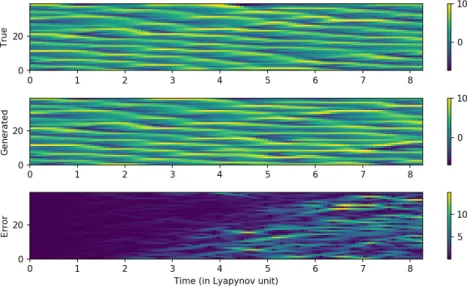
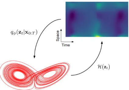
The first application is the identification of dynamical systems from noisy and partially observed data. We introduce a framework that merges classical data assimilation and modern deep learning to retrieve the differential equations that control the dynamics of the system. The role of the assimilation part in the proposed framework is to reconstruct the true states of the system from series of imperfect observations. Given those states, we then apply neural networks to identify the underlying dynamics. Using a state space for-mulation, the proposed framework embeds stochastic components to account for stochastic variabilities, model errors and reconstruction uncertainties. Experiments on chaotic and stochastic dynamical systems show that the proposed framework can remarkably improve the performance of state-of-the-art learning models on noisy and partial observations.

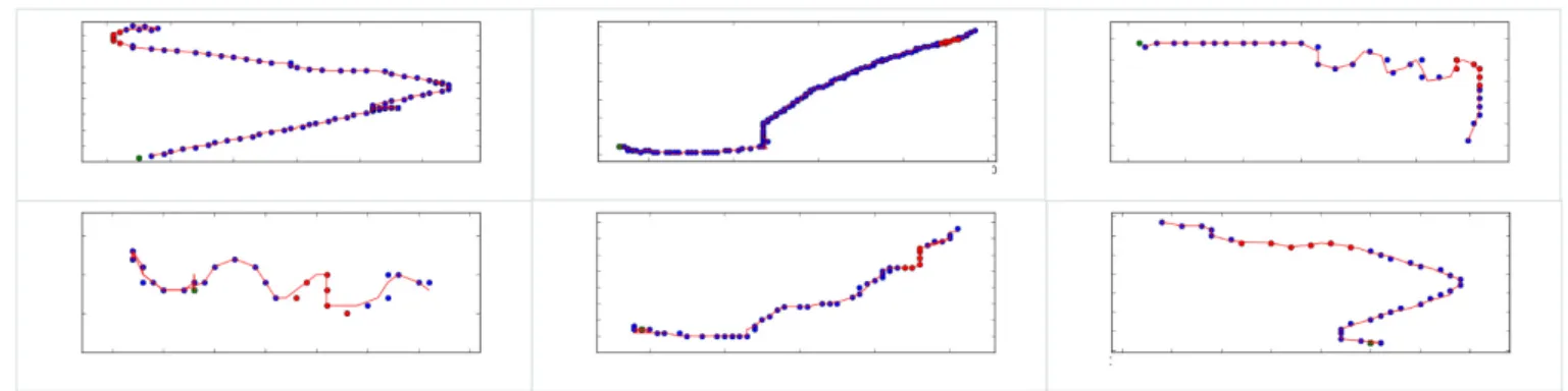
The second application is maritime traffic surveillance using AIS data. AIS is an automatic tracking system designed for vessels. The information richness of AIS has made it quickly become one of the most important sources of data in the maritime domain. However, AIS data are noisy, and usually irregularly sampled. We propose a multitask probabilistic deep learning architecture that can overcome these difficulties. Our model can achieve state-of-the-art performance in different maritime traffic surveillance related tasks, such as trajectory reconstruction, vessel type identification and anomaly detection, while reducing significantly the amount data to be stored and the calculation time. For the most important task—anomaly detection, we introduce a geospatial detector that uses variational deep learning to builds a probabilistic representation of AIS trajectories, then detect anomalies by judging how likely this trajectory is. This detector takes into account the fact that AIS data are geographically heterogeneous, hence the performance of the learnt probabilistic distribution is also geospatially dependent. Experiments on real data assert the relevance of the proposed method.

Key words: deep learning, variational inference, time series, state space model,

recur-rent neural network, dynamical system identification, anomaly detection, AIS, maritime traffic surveillance.

Résumé (Français)

Au cours des dernières décennies, l’augmentation de la quantité de données collectées a motivé l’utilisation d’approches basées sur les données. Cependant, la majorité des données disponibles sont non étiquetées, bruitées et peuvent être partiellement observées. De plus, beaucoup d’entre elles sont des séries temporelles, c’est-à-dire des données de nature séquentielle. Ce travail de thèse se focalise sur une classe de méthodes d’apprentissage profond, probabilistes et non-supervisées qui utilisent l’inférence variationnelle pour créer des modèles évolutifs de grande capacité pour ce type de données. Nous présentons deux classes d’apprentissage variationnel profond, puis nous les appliquons à deux problèmes spécifiques: l’apprentissage de systèmes dynamiques et la surveillance du trafic maritime.

La première application est l’identification de systèmes dynamiques à partir de données bruitées et partiellement observées. Nous introduisons un cadre qui fusionne l’assimilation de données classique et l’apprentissage profond moderne pour retrouver les équations différentielles qui contrôlent la dynamique du système. Le rôle de la partie d’assimilation, dans le cadre proposé, est de reconstruire les vrais états du système à partir des séries d’observations imparfaites. Étant donné ces états, nous appliquons ensuite des réseaux de neurones pour identifier la dynamique sous-jacente. En utilisant une formulation d’espace d’états, le cadre proposé intègre des composantes stochastiques pour tenir compte des variabilités stochastiques, des erreurs de modèle et des incertitudes de reconstruction. Des expériences sur des systèmes dynamiques chaotiques et stochastiques montrent que le cadre proposé peut améliorer remarquablement les performances des modèles d’apprentissage de pointe sur des observations bruitées et partielles.

La deuxième application est la surveillance du trafic maritime à l’aide des données AIS. L’AIS est un système de suivi automatique conçu pour les navires. La richesse d’informations de l’AIS en a rapidement fait l’une des sources de données les plus impor-tantes dans le domaine maritime. Cependant, les données AIS sont bruitées et généralement échantillonnées de manière irrégulière. Nous proposons une architecture d’apprentissage profond probabiliste multitâche capable de surmonter ces difficultés. Notre modèle peut atteindre des performances très prometteuses dans différentes tâches liées à la surveillance du trafic maritime, telles que la reconstruction de trajectoire, l’identification du type de navire et la détection d’anomalie, tout en réduisant considérablement la quantité de données à stocker et le temps de calcul. Pour la tâche la plus importante - la détection d’anomalie, nous introduisons un détecteur géospatialisé qui utilise l’apprentissage profond variationnel pour construire une représentation probabiliste des trajectoires AIS, puis détecter les anomalies en jugeant la probabilité de cette trajectoire. Ce détecteur prend

en compte le fait que les données AIS sont géographiquement hétérogènes, ce qui, par conséquet fait varier la qualité de la distribution probabiliste apprise. Des expériences sur des données réelles affirment la pertinence de la méthode proposée.

Mots clés: apprentissage profond, inférence variationnelle, séries temporelles, modèle

espace d’états, réseau de neurones récurrents, identification de systèmes dynamiques, détection d’anomalies, AIS, surveillance de trafic maritime.

Acknowledgement

The pursuit of a PhD is an enduring, yet exciting adventure in one’s life. And I consider myself lucky for having such great guidance and companionship from the following people.

Prof. Dung-Nghi Truong-Cong and Prof. Nhat-And Che-Viet, I would like to express my sincere gratitude for your help in the early days. I could not have embarked on this amazing journey without your unstinting support.

To my thesis supervisors: Prof. René Garello, Prof. Ronan Fablet, and Assoc. Prof. Lucas Drumetz, thank you for your leadership. René, your kindness, scientific feedback, and administrative support has helped me greatly throughout the way. Ronan, your knowledge was essential, your trust was crucial, and your patience was vital. You carved out the rough shape of this work and helped me turn it into something I can be proud of. Thank you also for always having an open door for me. You are a role model for me to look up to, and I am very fortunate to have worked with you. To Lucas, I credit those insightful comments and suggestions, especially during the phases of drafting and revising manuscripts.

Dr. Quang-Thang Nguyen and Dr. Alex TP Nguyen, special thanks for your mentorship and guidance. Whenever I need advice, I know that I can always count on you two. To Oscar Chapron, I have grown to love the Breton culture more thanks to you (I am reserving the best spot in my office for your Breton flag). Said Ouala, our late-night deadline running, the abroad missions, and the ups and downs we shared will be remembered. You are the best workmate, comrade, and friend (beside Oscar) that I could ask for.

During my PhD, I spent most of my time at the Department of Signal and Communi-cations (SC), IMT Atlantique. My gratitude goes to all my colleagues and the faculties members there. Prof. Aimee Johansen and Prof. Rebecca Clayton, thank you for your English courses and advice. Greatest thanks also to Monique Larsonneur and Martine Besnard for your keen support with various administrative tasks.

I would like to express my profound appreciation to Dr. Oliver S. Kirsebom, Fábio Frazão, and the PhD students at the Institute for Big Data Analytics (Dalhousie) for their unparalleled hospitality during the 2 internships I had there. And to Prof. Stan Matwin particularly for his kindness, his generosity, and the invaluable time he has spent on me. Prior to this PhD, I did an internship at Collecte Localisation Satellites (CLS). During this PhD, I had a special opportunity to come back and carry out a mission there. To people of CLS, especially to Dr. Guillaume Hadjuch, Rodolphe Vadaine and Dr. Vincent Kerbaol, I sincerely thank you for the opportunities and the collaboration.

I also would like to thank Prof. Steve Brunton for having sponsored my internship at the University of Washington.

I’m grateful to my thesis committee for their time examining my thesis manuscript, their invaluable remarks, and comments.

Finally, I would like to acknowledge the Mines-Télécom Foundation for their financial support during my undergraduate and my master. My PhD is support by public funds (Ministère de l’Education Nationale, de l’Enseignement Supérieur et de la Recherche,

FEDER, Région Bretagne, Conseil Général du Finistère, Brest Métropole), by Insti-tut Mines Télécom, received in the framework of the VIGISAT program managed by “Groupement Bretagne Télédétection” (BreTel).

List of publications

Journal papers

— D Nguyen, R Vadaine, G Hajduch, R Garello and R Fablet, GeoTrackNet-A

Maritime Anomaly Detector using Probabilistic Neural Network Representation of AIS Tracks and A Contrario Detection, IEEE Transactions on Intelligent Transportation

Systems (T-ITS), 2019.

— S Ouala, D Nguyen, L Drumetz, B Chapron, A Pascual, F Collard, L Gaultier and R Fablet, Learning Latent Dynamics for Partially-Observed Chaotic Systems, Chaos: An Interdisciplinary Journal of Nonlinear Science, 2020.

Preprints

— D Nguyen, S Ouala, L Drumetz and R Fablet, Variational Deep Learning for the

Identification and Reconstruction of Chaotic and Stochastic Dynamical Systems from Noisy and Partial Observations, 2020.

— D Nguyen, S Ouala, L Drumetz and R Fablet, EM-like learning chaotic dynamics

from noisy and partial observations, 2019.

Publications in conference proceedings

— D Nguyen, M Simonin, G Hajduch, R Vadaine, C Tedeschi and R Fablet, Detection

of Abnormal Vessel Behaviors from AIS data using GeoTrackNet: from the Laboratory to the Ocean, 21st IEEE International Conference on Mobile Data Management

(MDM), Maritime Big Data Workshop (MBDW), 2020.

— D Nguyen, S Ouala, L Drumetz and R Fablet, Assimilation-based Learning of

Chaotic Dynamical Systems from Noisy and Partial Data, 2020 IEEE International

Conference on Acoustics, Speech and Signal Processing (ICASSP), 2020.

— D Nguyen, OS Kirsebom, F Frazão, R Fablet and S Matwin, Recurrent Neural

Net-works with Stochastic Layers for Acoustic Novelty Detection, 2019 IEEE International

Conference on Acoustics, Speech and Signal Processing (ICASSP), 2019.

— D Nguyen, R Vadaine, G Hajduch, R Garello and R Fablet, A Multi-task Deep

IEEE International Conference on Data Science and Advanced Analytics (IEEE DSAA), 2018.

— D Nguyen, R Vadaine, G Hajduch, R Garello and R Fablet, An AIS-based Deep

Learning Model for Vessel Monitoring, NATO CMRE Maritime Big Data Workshop,

2018.

— S Ouala, D Nguyen, L Drumetz, B Chapron, A Pascual, F Collard, L Gaultier and R Fablet, Learning ocean dynamical priors from noisy data using assimilation-derived

neural nets, 2019 IEEE International Geoscience and Remote Sensing Symposium

(IGARSS), 2019.

— S Ouala, D Nguyen, SL Brunton, L Drumetz and R Fablet, Learning Constrained

Dynamical Embeddings for Geophysical Dynamics, Climate Informatics (CI), 2019.

Communications in international conferences

— D Nguyen, S Ouala, L Drumetz and R Fablet, Learning Chaotic and Stochastic

Dynamics from Noisy and Partial Observation using Variational Deep Learning, 10th

International Conference on Climate Informatics (CI), 2020.

— S Ouala, R Fablet, D Nguyen, L Drumetz, B Chapron, A Pascual, F Collard and L Gaultier, Data assimilation schemes as a framework for learning dynamical model

from partial and noisy observations, General Assembly of the European Geosciences

Union (EGU), 2019.

Acronyms

AIS Automatic Identification System AnDA Analog Data Assimilation ANN Artificial Neural Network CNN Convolutional Neural Network COG Course Over Ground

DAODEN Data-Assimilation-based Ordinary Differential Equation Network DBSCAN Density-Based Spatial Clustering of Applications with Noise DL Deep Learning

DSSM Deep State Space Model EKF Extended Kalman Filter ELBO Evidence Lower BOund EM Expectation-Maximisation EnKF Ensemble Kalman Filter EnKS Ensemble Kalman Smoother FIVO Filtering Variational Objective GMM Gaussian Mixture Model GRU Gated Recurrent Unit HMM Hidden Markov Model

IWAE Importance Weighted AutoEncoder KDE Kernel Density Estimation

KL divergence Kullback–Leibler divergence LGSSM Linear Gaussian State Space Model LSTM Long Short-term Memory

LVM Latent Variable Model MAP Maximum A Posteriori MDA Maritime Domain Awareness ML Machine Learning

MMSI Maritime Mobile Service Identity NLP Natural Language Processing NN Neural Network

ODE Ordinary Differential Equation PF Particle Filter

RK4 Runge-Kutta 4

RNN Recurrent Neural Network ROI Region Of Interest

SDE Stochastic Differential Equation SGD Stochastic Gradient Descent

SINDy Sparse Identification of Nonlinear Dynamics SOG Speed Over Ground

SRNN Stochastic Recurrent Neural Network SSM State Space Model

SVAE Sequential Variational AutoEncoder

TREAD Traffic Route Extraction and Anomaly Detection VAE Variational AutoEncoder

VDL Variational Deep Learning VI Variational Inference

VRNN Variational Recurrent Neural Network

Table of Contents

Summary (English) iii

Résumé (Français) v

Acknowledgement vii

List of publications ix

Acronyms xi

Table of Contents xiii

I

Introduction

1

1 General Introduction 3

1.1 Motivation . . . 3

1.2 Outline and contributions . . . 7

2 Variational Deep Learning for Time Series Modelling and Analysis 9 2.1 Latent variable models (LVMs) . . . 10

2.1.1 Motivation . . . 10

2.1.2 Variational inference (VI) . . . 11

2.1.3 Objective functions . . . 12

2.1.4 Optimisation methods . . . 13

2.1.5 Variational Auto-Encoders (VAEs) . . . 14

2.2 State space models (SSMs) . . . 17

2.2.1 Formulation . . . 17

2.2.2 Properties . . . 19

2.2.3 Posterior inference for SSMs . . . 20

2.2.4 Example: linear Gaussian SSMs (LGSSMs) . . . 21

2.3 Recurrent neural networks (RNNs) . . . 23

2.4 Variational deep learning for noisy and irregularly sampled time series modelling and analysis . . . 25

2.4.1 Deep state space models (DSSMs) . . . 25

TABLE OF CONTENTS

2.4.3 Handling irregularly sampled data . . . 31

2.5 Summary and discussion . . . 32

II

Variational Deep Learning for Dynamical System

Identification

35

3.2 Examples of dynamical systems . . . 39

3.2.1 The Lorenz-63 system . . . 39

3.2.2 The Lorenz-96 system . . . 40

3.2.3 The stochastic Lorenz-63 system . . . 41

3.3 Numerical methods for differential equations . . . 41

3.3.1 The Euler method . . . 42

3.3.2 The Runge-Kutta 4 method . . . 43

3.3.3 The Euler–Maruyama method . . . 44

3.4 Learning dynamical systems . . . 44

4 DAODEN 47 4.1 Introduction . . . 48

4.2 Problem formulation . . . 49

4.3 Related work . . . 50

4.4 Proposed framework . . . 52

4.4.1 Variational inference for learning dynamical systems . . . 52

4.4.2 Parametrisation of the generatvie model pθ . . . 54

4.4.3 Parametrisation of the inference model qφ . . . 55

4.4.4 Objective functions . . . 56

4.4.5 Optimisation strategies . . . 58

4.4.6 Random-n-step-ahead training . . . 59

4.4.7 Initialisation by optimisation . . . 61

4.5 Experiments and results . . . 62

4.5.1 Benchmarking dynamical models . . . 62

4.5.2 Baseline schemes . . . 63

4.5.3 Instances of the proposed framework . . . 64 xiv

TABLE OF CONTENTS

4.5.4 Evaluation metrics . . . 64

4.5.5 L63 case-study . . . 65

4.5.6 L96 case-study . . . 68

4.5.7 L63s case-study . . . 72

4.5.8 Dealing with an unkown observation operator . . . 73

4.6 Conclusions . . . 76

III

Variational Deep Learning for Maritime Traffic

Surveillance

77

5.2 AIS applications . . . 81

5.3 Challenges working with AIS . . . 83

6 MultitaskAIS 85 6.1 Introduction . . . 86

6.2 Related work . . . 87

6.3 Proposed multi-task VRNN model for AIS data . . . 88

6.3.1 A latent variable model for vessel behaviours . . . 89

6.3.2 “Four-hot” representation of AIS messages . . . 91

6.3.3 Embedding block . . . 92

6.3.4 Trajectory reconstruction submodel . . . 92

6.3.5 Abnormal behaviour detection submodel . . . 92

6.3.6 Vessel type identification submodel . . . 93

6.4 Experiments and Results . . . 94

6.4.1 Preprocessing . . . 94

6.4.2 Embedding block calibration . . . 95

6.4.3 Vessel trajectory construction . . . 96

6.4.4 Abnormal behaviour detection . . . 96

6.4.5 Vessel type identification . . . 100

6.5 Insights on the considered approach . . . 101

TABLE OF CONTENTS 7 GeoTrackNet 105 7.1 Introduction . . . 106 7.2 Related work . . . 108 7.3 Proposed Approach . . . 110 7.3.1 Data representation . . . 110

7.3.2 Probabilistic Recurrent Neural Network Representation of AIS Tracks111 7.3.3 A contrario detection . . . 114

7.4 Experiments and results . . . 116

7.4.1 Experimental set-up . . . 116

7.4.2 Experiments and results . . . 118

7.5 Conclusions and future work . . . 128

IV

Closing

133

8.2 Open questions and future work . . . 136

Appendices 139 A Variational Deep Learning for Acoustic Anomaly Detection 141 A.1 Introduction . . . 141

A.2 The proposed approach . . . 143

A.2.1 Recurrent Neural Networks with Stochastic Layers (RNNSLs) . . . 143

A.2.2 RNNSLs for Acoustic Novelty Detection . . . 144

A.3 Related work . . . 145

A.4 Experiment and Result . . . 147

A.4.1 Dataset . . . 147

A.4.2 Experimental Setup . . . 147

A.4.3 Results . . . 148

A.5 Conclusions and perspectives . . . 150

B Extended Abstract/Résumé Étendu 151 B.1 Apprentissage profond variationnel pour la modélisation et l’analyse de séries temporelles . . . 153

TABLE OF CONTENTS

B.1.1 Modèles de variable latente pour la modélisation et l’analyse de

séries temporelles . . . 154

B.1.2 Modèles probabilistes séquentiels profonds . . . 156

B.2 VDL pour l’identification de systèmes dynamiques . . . 157

B.3 VDL pour la surveillance du trafic maritime . . . 161

B.4 Conclusion et perspectives . . . 164

B.4.1 Conclusion . . . 164

B.4.2 Perspectives . . . 165

Part I

A PhD is a great time in one’s life to go for a big goal, an even small steps towards that will be valued.

Yoshua Bengio

Chapter 1

General Introduction

1.1

Motivation

The term “deep learning” (DL) was first introduced by Rina Dechter in 1986 (Dechter 1986). Nowaday, DL is usually understood as a family of machine learing (ML) methods that use artificial neural networks (ANNs) to learn features of data with multiple levels of abstraction (LeCun et al. 2015). Over the last decade, the world has witnessed an incredible development of DL. Machine learning in general, and deep learning in particular, have recently revolutionised many fields of research and application. In computer vision, DL has surpassed human-level performance for image classification, object detection, etc. (He

et al. 2015;Russakovsky et al. 2015). Many tasks that are hard to mathematically defined

such as mimicking an artistic style, generating artificial human-lookalike images, etc. have been achieved by neural-network-based (NN-based) models (I. Goodfellow, Pouget-Abadie,

et al. 2014; Zhu et al. 2017; Karras et al. 2019). In natural language processing (NLP),

the introduction of embedding models such as Word2Vec (Mikolov et al. 2013) and Glove

(Pennington et al. 2014), ELMo (Peters et al. 2018) and BERT (Devlin et al. 2018)

has significantly boosted the fields. NNs have helped create better machine translation

(Sutskever et al. 2014; Y. Wu et al. 2016), human-like chatbots (of which Apple’s Siri,

Google Assistant, and Amazon Alexa are great examples), fake news detection models

(Shu et al. 2017). From medicine, healthcare (Ravì et al. 2017; Esteva et al. 2019) to

Part I, Chapter 1 –General Introduction

et al. 2018), DL has yielded numerous state-of-the-art results and has been leveraged to

obtain better solutions for complex tasks.

Among many others, two main components that build the success of deep learning are rapid advances in computational power and the ever-increasing availability of data. New hardware technologies dedicated for parallel computing such as GPUs or TPUs allow training big deep neural networks within a reasonable time. Some models might take months to train in the past now can be trained in a few hours. Alongside with those hardware accelerators, open-source libraries such as Tensorflow (Abadi et al. 2016), Pytorch

(Paszke et al. 2017), MXnet (T. Chen et al. 2015), etc. have made DL more accessible.

Thanks to those libraries, students, researchers and deep learning practitioners can spend more time on ideas and algorithms instead of on implementation aspects. With the growing popularity of the Internet, the development of sensor technologies as well as the Internet of things (IoT), more and more data are collected. As a data-driven approach, DL models require representative data, both in quality and in volume to be effective. For example, the launch of the ImageNet challenge (Russakovsky et al. 2015) is one of the main factors that evoke the rebirth of deep learning, marked by the victory of AlexNet (Krizhevsky

et al. 2012). On the other hand, the success of DL encourages the collection of large data

sets, because we now can extract and exploit valuable information from data.

Although the above-mentioned results are fascinating and their potential are appealing, deep learning still has many drawbacks (Marcus 2018):

— Most of the successful NN-based practical applications use supervised learning methods. Supervised learning is a branch of machine learning where the data are labelled, the models aim to find a mapping that predicts the labels given the data as the input. However, unlike unlabelled data, which are highly available, labelled data are expensive to obtain. For this reason, DL community has recently focused more on unsupervised and semi-supervised learning (Diederik P. Kingma and

Welling 2013;Durk P. Kingma et al. 2014; Rezende, Mohamed, and Wierstra 2014;

Locatello et al. 2019; Yin et al. 2018;Zhou et al. 2017; Metz et al. 2018; Vacar et al.

2019). In unsupervised learning, the data are not labelled, the models aim to uncover the structures, the patterns, the correlations existing in data. Those discoveries can be used for semi-supervised learning, where the models aim to do supervised tasks with only a small part of the data is labelled.

— Neural networks naturally do not deal well with noisy and irregularly-sampled data. The lack of explicit mathematical models makes standard neural networks

1.1. Motivation such as multilayer perceptrons (MLPs), recurrent neural networks (RNNs),

convolutional neural networks (CNNs), etc. unable to distinguish noise from

data. They blindly apply a series of calculations on a set of numbers (the inputs) to provide another set of numbers (the outputs). Those may cause the models to overfit the training data, or to create unexpected effects such as the adversarial examples (I. Goodfellow, Pouget-Abadie, et al. 2014; I. J. Goodfellow et al. 2014;

Szegedy et al. 2014; Pajot et al. 2018). Because the calculations of DL models are

performed on computational graphs, they do not accept NaN (not a number) as an input. Hence, we usually have to perform a preprocessing interpolation to fill the missing data. This step prevents DL from achieving its own end-to-end learning goal. Almost all DL models thus far suppose that the data are sampled regularly. In the real-world, it is rarely the case for numerous applications.

— It is difficult to embed prior knowledge into neural networks. One of the ultimate goals of DL is to perform an end-to-end learning, which means to minimise the number of hand-engineering steps and to relax as much as possible weak hypotheses. However, for tasks that DL is still not doing well, one may not want to throw away domain expertise that has been studied and verified for decades. For example, it has been well known that many atmospheric processes are chaotic (Lorenz 1963;Lorenz 1996), yet embedding this knowledge into a neural network is not trivial.

In the last few years, variational deep learning (VDL)—a branch of deep learning, has arisen as a very promising candidate to overcome those difficulties (Diederik P.

Kingma and Welling 2013; Rezende, Mohamed, and Wierstra 2014). Broadly speaking,

VDL combines probabilistic modelling and deep learning to create flexible, high-capacity, expressive generative models that can scale easily. In this thesis, we focus on the sequential setting of VDL, applied to a type temporally-correlated data, called time series. We introduce two different classes of sequential VDL, then apply them to two different types of highly nonlinear, noisy and irregularly sampled time series data: observations of dynamical systems and maritime traffic data.

Three-quarter’s of the Earth’s surface is covered by water. Since the dawn of life, the ocean has evolved and interacted tightly with the planet and its climate. For humankind, the ocean has provided rich physical and biological resources, as well as a major transport medium. Nowadays, with the rising concern of climate change as well as the rapid growth of globalisation and global trade, the studies of oceanography and maritime traffic are attracting a lot of attention. Understanding the dynamics of the ocean helps forecast

Part I, Chapter 1 –General Introduction

weather condition, simulate climate change, evaluate the impact of waves and tides to the coastal areas, etc. Monitoring, analysing and modelling maritime traffic play an important role in maritime safety and security. Maritime traffic surveillance also contributes to

maritime domain awareness (MDA), fishing control and smuggling detection. To meet

the needs for oceanography and maritime traffic surveillance, maritime data are more and more collected. More sensors are placed in the ocean, on the surface (Sendra et al. 2015), along the coastline (Bresnahan et al. 2020) and especially in the sky (Biancamaria et al. 2016) to measure the ocean. For maritime traffic, the automatic identification system (AIS) provide a fine-grained, rich information source of data. Everyday, on a global scale there are hundreds of millions of AIS messages transmitted (Perobelli 2016). The huge amount of available data makes deep learning a plausible approach.

However, there are still many problems to tackle. Usually we do not have direct access to the true states of the ocean dynamics. Instead, we observe a series of damaged and potentially incomplete measurements. As mentioned above, DL does not deal well with this type of data. Nevertheless, the hidden processes of oceanographic data obey fundamental physical laws. This is again a drawback of deep learning. Similarly, AIS trajectories are just noisy, potentially irregularly-sampled observations of the underlying movement patterns of vessels. Without prior knowledge integrated, DL can hardly capture those patterns.

Conducted within the framework of ANR (French Agence Nationale de la Recherche) AI Chair OceaniX, this thesis aims to exploit deep learning for ocean sciences. Because maritime data are usually sequential, noisy and irregularly sampled, we focus on a family of sequential models which use variational inference to uncover the hidden dynamics of the learning data. We combine deep learning architectures with probabilistic models for time series, and integrate prior knowledge of the domain to create a novel framework for learning dynamical systems1 (Part II) and a novel deep learning model for maritime

surveillance using AIS data (Part III). The details will be presented in the next sections. This thesis work is supported by public funds (Ministère de l’Education Nationale, de l’Enseignement Supérieur et de la Recherche, FEDER, Région Bretagne, Conseil Général du Finistère, Brest Métropole); by ANR (French Agence Nationale de la Recherche), under grants Melody and OceaniX; and by Institut Mines Télécom, received in the framework of the VIGISAT program managed by “Groupement Bretagne Télédétection” (BreTel). It benefits from HPC and GPU resources from Azure (Microsoft EU Ocean awards) and

1. In this thesis we introduce this framework for the identification of general dynamical systems, some specific applications of this framework in geophysical oceanography are presented in our related work in

(Ouala, Duong Nguyen, Herzet, et al. 2019) and (Ouala, Duong Nguyen, Drumetz, et al. 2020).

1.2. Outline and contributions from GENCI-IDRIS (Grant 2020-101030). The work in Part III is supported by DGA (Direction Générale de l’Armement) and by ANR under reference ANR-16-ASTR-0026 (SESAME initiative).

The primary target audience of this thesis is DL practitioners whose research interests focus on geoscience, marine science and maritime traffic. We suppose that readers have enough background on dynamical system, AIS, probabilistic and deep learning.

1.2

Outline and contributions

This thesis contains three main parts. In the first part, we provide the motivation, the formulation and the construction of general variational deep learning (VDL) frameworks for time series analysis. This part aims to provide the “big picture” of different deep learning models for sequential data, how they are constructed and the relations between them. In the next parts, we present our models specifically designed for domain applications: dynamical system identification (Part II) and maritime traffic surveillance using AIS data (Part III). The details are as follows:

— In Part I (Chapter 2) we introduce two classes of deep latent variable models for sequential data: deep state space models (DSSMs) andsequential variational

autoencoders (SVAEs). We present the derivations of these models, starting from latent variable models (LVMs)—which are the bricks to build all the models in

this thesis—to their two sequential extensions: state space models (SSMs) and

recurrent neural networks (RNNs). DSSMs and SVAEs are then obtained by

combining them with variational deep learning, to help these models become more expressive and scalable.

— Part II (Chapter 3 and Chapter 4) contains paper (Duong Nguyen, Ouala, et al.

2020b) in which we present a DSSM, called data-assimilation-based ordinary

differential equation network (DAODEN), specifically designed for learning

dy-namical system. DAODEN uses state-of-the-art neural network architectures to model the dynamics of ordinary differential equations (ODEs) systems and possibly of

stochastic differential equations (SDEs) systems. DAODEN contains two key

components: an inference model that mimics classical data assimilation methods to reconstruct the true hidden states of the systems from noisy and potentially partial observations, and a generative model that use state-of-the-art neural networks representation of dynamical systems to retrieve the underlying dynamics of these

Part I, Chapter 1 –General Introduction

states. Therefore, by construction, DAODEN can obtain comparable performance with the one of models trained on ideal observations, even when DAODEN is trained on highly damaged data.

— Part III (Chapters 5, 6 and 7 ) contains papers (Duong Nguyen, Vadaine, et al.

2018; Duong Nguyen, Vadaine, et al. 2019; Duong Nguyen, Simonin, et al. 2020), in

which we present MultitaskAIS and GeoTrackNet. MultitaskAIS is a multitask deep learning architecture for maritime traffic surveillance using AIS data (Chapter 6). The core of this architecture is an SVAE, which converts noisy and irregularly sampled AIS messages into series of clean and regularly sampled hidden states of the vessel’s trajectory. These states then can be used for task-specific sub-models (such as trajectory reconstruction, vessel type identification, anomaly detection).

Experiments show that MultitaskAIS can achieve state-of-the-art performance on those takes, while requiring a significantly smaller storage and computational need. GeoTrackNet is the anomaly detection submodel of MultitaskAIS. This model takes into account the fact that the performance of a model that represents AIS trajectories are location-dependant to create a geospatially-sensitive detector that can effectively detect anomalies in vessels’ behaviour.

— Part IV (Chapter 7) finally summarises the contributions of this thesis, discusses the remain challenges and some directions for future work.

— The Appendix A is an application our idea for anomaly detection using VDL to acoustic anomaly detection in the appendix.

You never really understand a person until you consider things from his point of view... Until you climb inside of his skin and walk around in it.

Harper Lee

Chapter 2

Variational Deep Learning for

Time Series Modelling and Analysis

When we monitor or track a process, the sequences of the obtained observations are usually temporally correlated. This type of data is called time series. Modelling time series is a challenging task, because most of the time we do not know the governing laws that define the dynamics of the considered process. These laws can be highly nonlinear, chaotic and/or stochastic. Moreover, the data that we obtain may not be the true states of the process, but rather the noisy and partial observations/measurements. Over the last few years, sequential variational deep learning has emerged as a very promising approach for time series modelling and time series analysis (R. G. Krishnan et al. 2017;J. Chung et al.

2015; Fraccaro et al. 2016). This approach combines probabilistic modelling and deep

learning (usually RNN-based networks) to create high capacity, expressive models that can capture the stochasticities, variations, uncertainties and long-term correlations in the data. In this chapter, we will present the motivation, the formulation and the applications of this approach. The content presented here is the theory part of the applications in Part II and Part III.

Part I, Chapter 2 –Variational Deep Learning for Time Series Modelling and Analysis

2.1

Latent variable models (LVMs)

2.1.1

Motivation

Given a set of possibly high-dimensional observations X = {x(1)_{, ..x}(N )_{}, the goal}

of probabilistic unsupervised learning models is to learn a probability distribution p(x) that well describes X. Latent variable models (LVMs) introduce an unobserved latent

variable zthat helps model p(x). The joint distribution p(x, z) is then computed as:

p(x, z) = p(x|z)p(z), (2.1)

where p(z) is the prior distribution over z and conditional distribution p(x|z) is the

emission distribution over x, given z. The posterior distribution p(z|x) can be

computed using the Bayesian formula:

p(z|x) = p(x|z)p(z)

p(x) . (2.2)

If z is continuous, p(x) can be obtained by marginalising over z:

p(x) =

Z

p(x, z)dz =

Z

p(x|z)p(z)dz. (2.3)

For discrete variables, we replace the integration above by the sum over all possible value of

z. In this paper, we present only the formula for continuous variables, however, most of the

ideas also apply to the discrete case. We may also use discrete z for some demonstrating examples.

The underlying hypothesis of VLMs is in order to generate an observation x(s), we

first draw a sample z(s) from p(z), then use it to draw a new sample from the emission

distribution p(x|z(s)_{). There are different ways to interpret the latent variable z. For some}

applications, z is considered as the true physical event, of which x is just a corrupted observation. An example of this interpretation is the famous Kalman filter that was used in the Apollo project (Kalman 1960). Another way of interpreting z is that the latent variable allows us to factor the complex and possibly intractable distribution p(x) into more tractable distributions p(z) and p(x|z). For example, to generate a human portrait image x, the latent variable z may contain the gender, age, race of that human.

Latent variables have been widely used in statistics and in machine learning. Among 10

2.1. Latent variable models (LVMs) many famous others, we may name principal component analysis (PCA), mixture

models, hidden Markov models (HHMs), state space models (SSMs) (Bishop 2006), variational auto-encoders(VAEs) (Diederik P. Kingma and Welling 2013;Rezende and

Mohamed 2015). We will go through some of those models later in this thesis.

2.1.2

Variational inference (VI)

One of the main task in LVMS is to calculate the posterior distribution p(z|x). However, apart from a small set of simple cases, this distribution is intractable because the integral in Eq. (2.3) does not have an analytic solution. In such situations, we have to approximate

p(z|x). There are two classes of techniques for this approximation:

— Stochastic techniques: this class uses sampling techniques to generate an ensemble of points that represent the distribution to estimate. If the number of points is large enough, the approximations converge to the exact results. An example of the methods in this class is Gibbs sampling (Geman et al. 1984; Barbos et al. 2017;

Féron et al. 2016). However, those methods are computationally expensive and do

not scale well to large data sets.

— Deterministic approximation techniques: this class uses analytical approximations to p(z|x). They impose the assumption that the posterior comes from a particular parametric family of distributions or that it factorises in a certain way. These methods scale very well, however, they never generate the exact results. An example of the methods in this class is variational inference (Blei et al. 2017), which is the topic of this section.

Recall that the objective is to find the distributions of two variables x and z that maximise the likelihood of the set of observations X. In practice, we usually use log pθ(X)

instead of pθ(X) to leverage some nice properties of the log function and to avoid problems

with very small numbers in numerical implementation. We focus on a family of distribution

Part I, Chapter 2 –Variational Deep Learning for Time Series Modelling and Analysis

decompose log pθ(x) as follows:

log pθ(x) = Z q(z) log pθ(x)dz (2.4) =Z q(z) logpθ(x, z) pθ(z|x) dz (2.5) =Z q(z) logpθ(x, z)q(z) pθ(z|x)q(z)dz (2.6) =Z q(z) logpθ(x, z) q(z) dz + Z q(z) log q(z) pθ(z|x) dz (2.7) = Eq(z) " pθ(x, z) q(z) # + KL [q(z)||pθ(z|x)] , (2.8)

with KL [q||p] denotes the Kullback–Leibler divergence between two distributions q and p. Because the KL divergence is a non-negative quantity, the first term in the right hand side of Eq. (2.8), denoted as L(x, pθ, q), is a lower bound of log pθ(x). L(x, pθ, q) is called the

evidence lower bound (ELBO). Variational inference (VI) suggests approximating

the intractable quantity log pθ(x) by L(x, pθ, q). The error of this approximation, i.e. the

difference between log pθ(x) and L(x, pθ, q) is KL [q(z)||pθ(z|x)]. Hence, to find log pθ(x),

we minimise KL [q(z)||pθ(z|x)] w.r.t. q(z). Because L(x, pθ, q) = log pθ(x) if and only

if q(z) = pθ(z|x), a natural choice for q is q(z) = q(z|x). In other words, VI converts

an intractable inference problem to an optimisation problem by approximating the true posterior distribution pθ(z|x) by the variational distribution q(z|x).

Note that those above are correct for any arbitrary q. Hence to make a good approxi-mation, we should choose q(z|x) high capacity enough, as long as the ELBO is tractable. In this thesis, we focus on a family of distributions qφ that can be parameterised by a set

of parameters φ.

2.1.3

Objective functions

The goal of probabilistic unsupervised learning is to maximise log pθ(X). In Section

2.1.2 we introduced the ELBO, which is an lower bound of log pθ(X), as an objective

function for the learning. Many efforts have been conducted to tighten this bound. Among them, we might cite the importance weighted auto-encoder (IWAE) bound (Burda

et al. 2016) and the fitering variational objective (FIVO) (Maddison et al. 2017),

which is used for sequential data. The idea is instead of drawing only one sample from

qφ(z|x), we draw N samples then average the importance-weighted results. These methods

2.1. Latent variable models (LVMs) guarantee that the bounds are tighter than the ELBO. However, on one hand, they use more computational resources. On the other hand, tighter variational bounds are not necessarily better (Rainforth et al. 2018). For the applications in this thesis, we empirically observed that the trade-off is not worth, hence we do not present IWAE and FIVO here. Another example of using loose lower bounds is maximum a posteriori (MAP) inference. Instead of estimating a distribution for the latent variable z, MAP inference computes only the single most likely value:

z∗ = argmax

z

qφ(z|x). (2.9)

In the context of VI, the MAP solution can be explained as the case where q is parameterised by Dirac delta functions. Although the MAP bound is infinitely loose, MAP inference is still very common (Bishop 2006).

2.1.4

Optimisation methods

Given an objective function L(x, θ, φ) (ELBO, IWAE, FIVO, MAP solution, etc.) as presented in Section 2.1.3, the next step is to optimise this quantity over the observations w.r.t. θ and φ. In this section, we present two strategies to perform this optimisation: i) alternatively optimise L over θ and φ using the expectation-maximisation (EM) algorithm and ii) simultaneously update θ and φ using the gradient of L.

Expectation–maximisation (EM) algorithm

The expectation-maximisation algorithm is an iterative optimisation technique for LVMs (Dempster et al. 1977;C. J. Wu 1983; Neal et al. 1998). Starting from the initial condition θ(0) _{and φ}(0)_{, each iteration i in EM contains two steps:}

— In the E step, φ is updated to maximise L: φ(i) _{= argmax}

φ

L(θ(i−1), φ). This step

corresponds to finding the true posterior distribution pθ(z|x) (because L is maximised

when qφ(z|x) = pθ(z|x)).

— In the M step, θ is updated, while φ is held fixed: θ(i) _{= argmax}

θ

L(θ, φ(i)_{). This}

step corresponds to increasing the objective function L.

EM has some nice properties, such as the convergence is fast and guaranteed1 (

Ghahra-mani and Roweis 1999). However, EM may not apply for very general configurations,

Part I, Chapter 2 –Variational Deep Learning for Time Series Modelling and Analysis

because the inference problem may not be tractable when considering complex dependence structure.

Gradient-based techniques

Another strategy to optimise L is to update θ and φ simultaneously using the gradient of L. This approach is widely used for neural networks. For example, in the current context, we can update {θ(i)

, φ(i)} using a gradient ascent technique:

{θ(i), φ(i)}= {θ(i−1), φ(i−1)}+ η∇{θ,φ}L(x, θ, φ). (2.10)

with η is the learning rate.

Because maximising L is equal to minimising −L, we can re-write Eq. (2.11) as follows:

{θ(i)_{, φ}(i)_{}= {θ}(i−1)_{, φ}(i−1)_{} − η∇}

{θ,φ}(−L(x, θ, φ)). (2.11)

The second notation, called gradient descent, is more common.

In deep learning, we usually use a “stochastic version” of Eq. (2.11). In each iteration, instead of evaluating ∇{θ,φ}−L(x, θ, φ) on the whole observation set X, we calculate this

quantity on just a subset of X, called mini-batch. This technique is known as stochastic

gradient descent (SGD) (Bottou et al. 2018). SGD is the basic form of gradient-based

optimisation techniques used in DL, many variants and extensions of SGD, such as AdaGrad (Duchi et al. 2011), RMSprop (G. Hinton 2012), Adam (Diederik P. Kingma and

Ba 2015), have been proposed to improve the performance of the learning. These methods

have been widely available in open-source DL frameworks such as Tensorflow (Abadi et al. 2016), Pytorch (Paszke et al. 2017).

2.1.5

Variational Auto-Encoders (VAEs)

So far we have reviewed LVMs and how to overcome the intractable inference problem in LVMs using VI. In this section, we present a class of LVMs that is extremely popular in probabilistic DL: the variational auto-encoders (VAEs) (Diederik P. Kingma and

Welling 2013; Rezende, Mohamed, and Wierstra 2014). VAEs are used as bricks to build

many generative models.

The architecture of VAEs is the basic form of VLMs, as show in Fig. 2.1. We have the observed variable x, the latent variable z, the emission distribution pθ(x|z) and the

2.1. Latent variable models (LVMs)

Figure 2.1 – Graphical model of a VAE. x is the observed variable, z is the latent variable. In this thesis, we use circle-shaped units for random variables, blue colour for observed variables, yellow colour for latent variables, red arrows for emission models and blue arrows for inference models.

variational distribution qφ(z|x) that approximates the true posterior distribution. Again,

in this thesis we focus on parametric models.

To build a VAE, there are three problems to deal with: i) how to define x and z, ii) how to define the emission model pθ(x|z) and iii) how to define the inference model qφ(x|z).

Most of the time we x is what we observe. e.g. the value of the pixels in an digital image, the temperature indicated by a thermometer in the room, etc. However, in some cases, we can use prior knowledge to convert observed data into another domain that is believed to be more suitable for the considered problem. For example, we can convert an audio record to a spectrogram to highlight some important features in the frequency domain. In this case, x is the spectrogram of the audio signal. The “four-hot vector” presented in Chapter 6 and Chapter 7 of this thesis is a specific representation we designed for AIS. As presented in Section 2.1.1, the interpretation of z is heavily context-dependent. For example, to generate an human portrait image, z can be the distance between two eyes, the colour of the skin, the ratio of the width to the length of the face, etc. If we do not have any prior knowledge of z, we usually model z as a continuous variable, whose prior is an isotropic multivariate Gaussian with mean 0 and covariance matrix I.

pθ(z) = N (0, I). (2.12)

Other distributions can also be used. However, unless we have prior knowledge of z, we should avoid multimodal distributions whose modes are sufficiently widely separated. To understand the reason behind it, let’s rewrite the ELBO as follows:

Part I, Chapter 2 –Variational Deep Learning for Time Series Modelling and Analysis

Figure 2.2 – The over concentration problem of minimising KL(q||p). When p is a multi-modal distribution, the optimisation might result in a distribution q that corresponds to only one mode of p.

Hence, to maximise L(x, pθ, qφ), we have to simultaneously maximise Eqφ(z|x)[pθ(x|z)]

and minimise KL [qφ(z|x)||pθ(z)] w.r.t. qφ. Minimising KL [qφ(z|x)||pθ(z)] means choosing

qφ(z|x) that has low probability wherever pθ(z) is small. If pθ(z) is a multimodal distribution

that has sufficiently widely separated modes, qφ(z|x) might just choose one of those modes,

as shown in Fig. 2.2

Given this distribution, we define a sufficiently complicated function that maps z to x. This mapping is called the decoder. In DL, the emission distribution pθ(x|z) is usually

modeled by a Gaussian distribution (for real-valued x) or a Bernoulli distribution (for binary z), whose parameters are computed by a neural network. For example:

pθ(x|z) = N (µx|z, Σx|z). (2.14)

with

µ_x|z, Σx|z= NNdecoder(z). (2.15)

Because we can not find the inverse function of the neural network NNdecoder, the

inference pθ(z|x) is intractable. As presented in Section 2.1.2, we will approximate this

posterior distribution by a variational distribution q, using some hypotheses, such as qφ is

a factorial distribution: qφ(z|x) = Y i qφ(zi|x). (2.16) 16

2.2. State space models (SSMs)

Figure 2.3 – Graphical model of an SSM. We use black arrows for transition models.

This technique—called the mean field technique, is widely used to simplify the behavior of high-dimensional stochastic models (Landau 1937; Flory 1942; Huggins 1941).

In DL, we usually use another network to model the mapping from x to z, called the

encoder:

qφ(z|x) = N (µz|x, Σz|x). (2.17)

with

µ_z|x, Σz|x = NNencoder(x). (2.18)

The parameters of the encoder and the decoder are then optimised using gradient-based techniques with an objective function presented in Section 2.1.2.

2.2

State space models (SSMs)

In the previous section, we assume that the observations are independent and

identically distributed (i.i.d). However, in the real world, there are many situations

where there is a temporal correlation in the data, for example, the measurements of the temperature at a particular place in two days, or two words in a sentence, are related. Such data are called time series. In this section, we introduce a way to model this type of data, especially how to model the temporal correlation in time series.

2.2.1

Formulation

A regularly-sampled time series x0:T is a sequence of T +1 observations: x0:T ∆

= {xt0, .., xtT}, where tk refers to the time sampling. We consider cases where the

sam-pling is regular: tk= t0+ k.δ with δ is the sampling resolution. For the sake of simplicity,

from now on in this thesis, unless specified otherwise we use the notation xk for xtk and

Part I, Chapter 2 –Variational Deep Learning for Time Series Modelling and Analysis

of xk, or entire xk may be missing.

Given an observed time series of observations x0:T, we aim to find a model that

maximise the likelihood:

pθ(x0:T) = pθ(x0) N Y k=1 pθ(xk|x0:k−1). (2.19) If we assume that: pθ(xk|x0:k−1) = pθ(xk|xk−1) (2.20)

then we have a first-order Markov model. In other words, in a first-order Markov model, the future states depend only on the present state. Generally, an nth_{-order Markov}

model assumes pθ(xk|x0:k−1) = pθ(xk|xk−n:k−1). At first glance, Eq. (2.20) looks like a

strong assumption, however, any nth_{-order Markov model can be converted to a first-order}

Markov model by using an augmented state: xaug

k = {xk, xk−1, .., xk−n+1}.

Although Markov models may look appealing, they are not really useful to directly model x0:T because the process of {xk}may not follow the Markov assumption to any order.

With the spirit of LVMs, we suppose that the data generating process of x0:T depends on a

series of latent variables z0:T. For example, let xkbe the values of a thermometer measuring

the temperature in a room, these values maybe effected by the errors in the sensor of the thermometer, hence we can not find the direct relation between two consecutive values

xk, xk+1. In this case, z can be the true temperature of the room, and there is a direct

relation, which is the heat equation, between two consecutive values of zk, zk+1.

The joint distribution can be factorised as:

pθ(x0:T, z0:T) = pθ(x0:T|z0:T)pθ(z0:T). (2.21)

The likelihood of the observation can be obtained by marginalising the latent variables:

pθ(x0:T) =

Z

pθ(x0:T, z0:T)dz0:T. (2.22)

Again, in general this integral is intractable. To compute pθ(x0:T), we have to impose

some hypotheses and some assumptions on the relation of x0:T and z0:T. One way of doing

so is using state space models (SSMs). The general form of an SSM is expressed as 18

2.2. State space models (SSMs) follow2:

zk∼ pθ(zk|zk−1) (2.23)

xk∼ pθ(xk|zk) (2.24)

with pθ(zk|zk−1) is the transition distribution (or prior distribution), models the

temporal evolution of zk, and pθ(xk|zk) is the emission distribution (or the observation

distribution), models the observation operator. The graphical model of an SSM is shown

in Fig. 2.3. Note that the distributions in Eqs. (B.6) and (B.7) are general, they include Dirac delta functions that model cases where zk is deterministic.

In order to determine pθ, SSMs use some characteristics presented in the following

sections.

2.2.2

Properties

Using the d-separation criterion, we derive some important properties of SSMs are as follows:

— The process of {zk}is Markovian, i.e. the future states depend only on the current

state zk.

— Given zk, xkdoes not depend on other states or observations: pθ(xk|x0:k−1, xk+1:T, z0:T) =

pθ(xk|zk).

— The process of {xk} is not Markovian, i.e. the future observation xk+1 depends on

the present and all the past observations x0:k.

Hence, the joint distribution in SSMs can then be factorised as:

pθ(x0:T, z0:T) = pθ(z0:T)pθ(x0:T|z0:T) = pθ(z0) T Y k=1 pθ(zk|zk−1) T Y k=0 pθ(xk|zk). (2.25)

Depending on the form of the transition and the emission distributions, a particular SMM may have other properties, which could be used to design particular models. For examples, if the latent variables zk are discrete, we can use hidden Markov models

(HMMs) (Rabiner 1989), Kalman filters (Kalman 1960) are designed for SSMs whose the transition and the emission distributions are Gaussian.

Part I, Chapter 2 –Variational Deep Learning for Time Series Modelling and Analysis

2.2.3

Posterior inference for SSMs

According to the Bayesian rule, given the whole sequence, the form of the posterior inference for SSMs is expressed as follows:

pθ(z0:T|x0:T) =

pθ(x0:T|z0:T)pθ(z0:T)

pθ(x0:T)

. (2.26)

In practice, we are usually interested in the following three inference problems:

— Filtering: zk is inferred using the all the present and the past observations; i.e., to

we compute pθ(zk|x0:k).

— Smoothing: using the d-separation criterion, zk depends not only on the current

and the past observations but also on the future observations, hence we compute

pθ(zk|x0:T). Because smoothing uses more information from data than filtering, it

should provide a better inference. However, smoothing requires information from the future, hence there is always a lag. On the other hand, filtering can be computed online.

— Prediction: we use the current and the past information to predict the future states,

i.e. to compute pθ(zk+1|x0:k).

When the transition and the emission are linear and Gaussian, the Kalman filter

(Kalman 1960) provides a mathematically elegant solution for the inference problem.

However, when the transition and/or the emission are not linear and Gaussian anymore, the posterior becomes intractable. We have to perform some approximations. For cases where the transition and the emission can be described by differentiable functions, the extended

Kalman filter (EKF) (Smith et al. 1962) approximates the posterior by a linearisation

of pθ(zk|zk−1) and pθ(xk|zk). The particle filter (Doucet et al. 2009) has a different

approach. This method uses sequential important sampling to recursively approximate

pθ(z0:k|x0:k) given pθ(z0:k−1|x0:k−1). In particle filters, a distribution is represented by a

set of particles. The ensemble Kalman filter (EnKF) (Evensen 2003) bridges the idea of the Kalman filter and the particle filter by supposing that the distributions represented by the particles are Gaussian. Each of those methods also has a corresponding smoothing version.

2.2. State space models (SSMs)

2.2.4

Example: linear Gaussian SSMs (LGSSMs)

To better understand SSMs, let’s revisit one of the most classic SSMs: the Kalman filter (Kalman 1960).

Consider a system governed by the following equations:

zk = Akzk−1+ ωk, (2.27)

xk = Hkzk+ υk. (2.28)

where Ak is a matrix, defines the transition of the hidden state zk; Hk is an invertible

matrix, defines the observation operator which maps the state zk to the observation xk

at each timestep k. ωk is the process noise, follows a zero-mean multivariate Gaussian

N(0, Q_k) and υk is the observation noise, follows another zero-mean multivariate Gaussian

N(0, Rk). All ωk and υk are mutually independent. The covariance matrices Qk and

Rk are called the model error and the observation error, respectively. Using the linear

transformation properties of Gaussian random variables, we can re-write Eqs. (2.27) and (2.28) as:

zk∼ pθ(zk|zk−1) = N (Akzk−1, Qk), (2.29)

xk∼ pθ(xk|zk) = N (Hkzk, Rk). (2.30)

here θ is the set {Ak, Hk, Qk, Rk}. Because the relationships between zkand zk−1, between

xk and zk are linear, and the two distributions pθ(zk|zk−1), pθ(xk|zk) are Gaussian, this

model is called a linear Gaussian SSM (LGSSM). The joint distribution of a LGSSM is factorised as:

pθ(x0:T, z0:T) = pθ(z0) T Y t=1 N(zk; Akzk−1, Qk) T Y t=0 N(xk; Hkzk, Rk). (2.31)

To find the inference distribution pθ(z0:T|x0:T), Kalman proposed a recursive algorithm

to compute the marginal posterior distribution pθ(zk|x0:k) at each timestep k, given the

Part I, Chapter 2 –Variational Deep Learning for Time Series Modelling and Analysis

Using Bayes’ rule and the independence properties of SSMs, we have:

pθ(zk|x0:k) = pθ(zk|xk, x0:k−1) (2.32) = pθ(xk|zk, x0:k−1)pθ(zk|x0:k−1) pθ(xk|x0:k−1) (2.33) = pθ(zk|x0:k−1) pθ(xk|zk) pθ(xk|x0:k−1) . (2.34)

Eq. (2.34) show that to calculate pθ(zk|x0:k), we first calculate pθ(zk|x0:k−1), i.e. to

predict zk using historical information in x0:k−1 (prediction step), then “correct” this

prediction using the information provided by xk (measurement step).

Suppose pθ(zk|x0:k) = N (µk, Σk) and pθ(zk|x0:k−1) = N (µk|k−1, Σk|k−1) . Lets compute

each component in Eq. (2.34) step by step. We have: pθ(zk|x0:k−1) ∆ = N (µk|k−1, Σk|k−1) (2.35) =Z pθ(zk|zk−1, x0:k−1)pθ(zk−1|x0:k−1)dzk−1 (2.36) =Z pθ(zk|zk−1)pθ(zk−1|x0:k−1)dzk−1 (2.37) =Z N(Akzk−1, Qk)N (µk−1, Σk−1)dzk−1 (2.38) = N (Akµk−1, AkΣk−1ATk + Qk). (2.39)

Note that (2.38) to (2.39) is possible because the model is linear and Gaussian.

Appling Bayes’ rule for the Gaussian pθ(xk|zk) = pθ(xk|zk, x0:k−1) (Murphy 2012), we

have:

Σ−1_k = Σ−1_k|k−1+ HTR−1H, (2.40)

µ_k = ΣkHR−1k xk+ ΣkΣ−1_k|k−1µk|k−1. (2.41)

Applying the matrix inversion lemma (Murphy 2012) for Σ−1

k , we have:

Σk = (I − KkHk)Σk|k−1, (2.42)

with Kk

∆

= Σk|k−1HTk(HkΣk|k−1HTk + Rk)−1 is the Kalman gain matrix.