HAL Id: hal-01380379
https://hal.archives-ouvertes.fr/hal-01380379
Submitted on 13 Oct 2016
HAL is a multi-disciplinary open access
archive for the deposit and dissemination of
sci-entific research documents, whether they are
pub-lished or not. The documents may come from
teaching and research institutions in France or
abroad, or from public or private research centers.
L’archive ouverte pluridisciplinaire HAL, est
destinée au dépôt et à la diffusion de documents
scientifiques de niveau recherche, publiés ou non,
émanant des établissements d’enseignement et de
recherche français ou étrangers, des laboratoires
publics ou privés.
Distributed under a Creative Commons Attribution| 4.0 International License
Fluid Forces on a Circular Cylinder Moving
Transversely in Cylindrical Confinement: Extension of
the Fritz Model to Larger Amplitude Motions
Cédric Leblond, Jean-François Sigrist, Christian Laine, Bruno Auvity, Hassan
Peerhossaini
To cite this version:
Cédric Leblond, Jean-François Sigrist, Christian Laine, Bruno Auvity, Hassan Peerhossaini. Fluid
Forces on a Circular Cylinder Moving Transversely in Cylindrical Confinement: Extension of the Fritz
Model to Larger Amplitude Motions. 2006 ASME Pressure Vessels and Piping Division Conference,
Jul 2006, Vancouver, Canada. pp.63 - 72, �10.1115/PVP2006-ICPVT-11-93051�. �hal-01380379�
FLUID FORCES ON A CIRCULAR CYLINDER MOVING TRANSVERSELY IN
CYLINDRICAL CONFINEMENT: EXTENSION OF THE FRITZ MODEL TO LARGER
AMPLITUDE MOTIONS
Cedric Leblond
Service Technique et Scientifique DCN Propulsion
Indret - BP 30
44620 LA MONTAGNE, FRANCE Email: cedric.leblond@dcn.fr
Jean Francois Sigrist Christian Laine
Service Technique et Scientifique DCN Propulsion Indret - BP 30 44620 LA MONTAGNE, FRANCE Bruno Auvity Hassan Peerhossaini Laboratoire de Thermocinetique CNRS UMR 6607 Rue C. Pauc - BP 50609 44306 NANTES, FRANCE ABSTRACT
This paper is related to the fluid forces prediction on a rapidly moving circular cylinder in cylindrical confinement. The Fritz model, which mainly assumes infinitesimal motions of the inner cylinder in an inviscid fluid, is one of the simplest model available in the scientific literature and is often used by design engineers in the nuclear industry.
In this paper, simple non-linear expressions of fluid forces are derived for the case of finite amplitude motions of the inner cylinder. Assuming a potential flow, advection term and geomet-rical deformations can be taken into account. The problem, for-mulated as a boundary-perturbation problem, is solved thanks to a regular expansion. The range of validity of the approximate analytical solution thus obtained is theoretically discussed. The results are also confronted to numerical simulations, which al-lows to emphasize some limits and advantages of the analytical approach.
NOMENCLATURE
(x, y)(ex,ey) Cartesian coordinates system.
(r,θ)(e
r,eθ) Polar coordinates system.
ρ Fluid density.
C
(t) Inner circular cylinder. Ψ Parametric curbe ofC
(t).R1 Inner circular cylinder radius.
R2 Outer circular cylinder radius.
α Cylinder radius ratio R2/R1.
n Exact outward normal to inner cylinder.
n0, n1, n2 Approximate outward normals to the inner cylinder
respectively at leading order, first order and second order.
e(t), ˙e(t), ¨e(t) Displacement, velocity and acceleration im-posed to the inner circular cylinder.
ξ Ratio between the maximum displacement of the inner cylin-der emaxand the radial clearance R2−R1,ξ= emax/(r2−R1)
rc Exact inner circular position.
r0, r1, r2 Approximate inner circular cylinder positions at lead-ing order, first order and second order.
u Local fluid velocity.
u0, u1, u2 Approximate velocity at leading order and velocity
rectification of first and second order.
p Local pressure.
p0, p1, p2 Approximate pressure at leading order, and first and second order rectifications.
Φ Velocity potential.
Φ0,Φ1,Φ2 Approximate velocity potentials at leading order, and first and second order rectifications.
ds Infinitesimal element of the curvilign abscissa of
C
(t).F
(t) Integrated force on the inner cylinder.INTRODUCTION
When a moving body is submerged, it can experience strong forces induced by the surrounding fluid. Since the body motion modifies the fluid flow, and the fluid flow can modify the body motion, this is a non-linear fluid/structure interaction problem. Furthemore, the induced fluid forces are not only functions of the whole history of the solid motion, which is sometimes deter-mined, but also of the ambiant perturbation level. Hence, it can be helpful to isolate physical phenomena in simple cases so as to identify their influences. Once it is done, models may be built and used to interpret real or numerical experiments. Moreover, if they are validated, they can avoid the use of a numerical code to solve the fluid domain in fluid/structure interaction problems.
This paper focuses on the fluid forces experienced by a rapidly moving circular cylinder in a annular fluid region. The motion is assumed radial, unidirectional and without rotation. It is related to a study whose aim is to predict impulsive fluid loads on naval components during a typical military shock. The sim-plest and most currently used model available in the scientific lit-terature related to this geometry is the Fritz one [1]. This model makes the following assumptions:
(i) the flow is two-dimensional, (ii) the flow is incompressible, (iii) the fluid is initially at rest, (iv) the fluid is inviscid,
(v) the advection term u ·∇u can be neglected,
(vi) the displacement imposed to the inner cylinder is very small compared to its radius : e(t)/R1<< 1.
Assumptions (i) to (iv) are also made in this paper. (i) is valid if the length of the cylinders is much longer than their radius, if there is no axial flow and if the two-dimensional flow is stable - or the effects of three-dimensional instabilities are negligible in the forces compared to potential effects. Some cases where hypothesis (ii) is not allowed are discussed in a companion paper [2] and more generally in [3,4]. Hypothesis (iii) can be relaxed in this study to an initially irrotational flow. Assumption (iv) is only roughly valid if the inner cylinder displacements are sufficiently small so that no separation occurs and if the motions are rapid enough to produce boundary layers [5] whose thickness are much thinner than the radial clearance and more specifically for high numberωR2
1(α− 1)
2/ν [4, 6]. This paper puts the focus on the relaxation of (v) and (vi). Hence the advection term is taken into account and the fluid force is expected to be valid, as it will be seen later, when the relation (e(t)/R1)3<< 1 is satisfied, which is less restrictive than that of (vi). Another way of thinking large displacements effects can be found in [7, 8].
In the first section the problem is formulated as a boundary-perturbation problem [9] for the velocity potential and a regular expansion method used to solve it analytically is exposed. The resolution up to the second order is achieved in the second sec-tion where the local pressure, velocity and integrated forces are
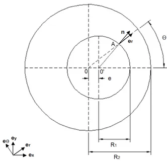
Figure 1. THE GEOMETRICAL CONFIGURATION.
given. In the third section, these results are compared with those obtained from a CFD code [10] based on a finite-volume dis-cretization on a moving mesh. Some conclusions are given in the last part.
PROBLEM FORMULATION General equations
With assumptions (ii) and (iv) of the last section, the Navier-Stokes equations governing the fluid motion are reduced to:
∂u
∂t + (u ·∇) u = −
1
ρ∇p (1)
∇· u = 0 (2) Since the fluid is inviscid and the density is constant, the Kelvin theorem1 can be used and provides the classical consequence: an inviscid fluid initially irrotational remains irrotational at latter times:
∇× u = 0 (3) Hence, there exists a function Φ, called the velocity potential, such that:
u =∇Φ (4)
Introducing it in Eqn. (2) gives the equation satisfied byΦin the fluid domain:
∇2Φ= 0 (5)
which is the Laplace equation. This derivation is classical and can be found in all fluid dynamics books (see [11] for example).
1the circulation on all closed material line is conserved [11].
Since the fluid is assumed inviscid, only the normal component of the velocity has to be conserved on the solid boundaries. For the geometry of interest in this paper (see Fig. 1), the boundary conditions in term of velocity potentiel are:
∇Φ· n = 0 on the fixed outer cylinder (6)
∇Φ· n = ˙e(t)ex· n on the moving inner cylinder (7)
In order to make this problem analytically tractable, the inner cylinder position and the unit outward normal n have to be ex-pressed in explicit terms in Eqn. (7). This is done in the following subsection.
Geometrical considerations
By considering the triangle OO0A in Fig. 1, it is
straightfor-ward to find that the inner circular cylinder position rc satisfies the following relation:
R21= r2c+ e2(t) − 2rce(t) cosθ (8) Since we are interested by motions of the inner cylinder much smaller than its radius, the physical solution of Eqn. (8) is:
rc(θ,t) = e(t) cosθ+ R1 s 1 −e 2(t) R21 sin 2θ (9)
This is the polar equation of the inner cylinder
C
(t). Expandingthe square root in terms of series gives
rc(θ,t) = R1 µ 1 + cosθe(t) R1 (10) + ∞
∑
n=1 (−1)n(sinθ)2n 1 n! n−1∏
k=0 µ 1 2− k ¶ µ e(t) R1 ¶2n!which always converges for |e(t)/R1| < 1. Thanks to this for-mula, we define approximate positions of the inner cylinder:
r0(θ) = R1 (11) r1(θ) = R1 µ 1 + cosθe(t) R1 ¶ (12) r2(θ) = R1 Ã 1 + cosθe(t) R1 −1 2sin 2θ µ e(t) R1 ¶2! (13) The boundary condition Eqn. (7) will be expressed thanks to this formula. r0 is used in the Fritz model and is the leading order approximation of Eqn. (10). r1and r2, respectivily the first and second order approximations of Eqn. (10), will be used to locate
C
(t) in the first order and second order models. It is also ofinterest to write in explict terms the unit outward normal n on the moving inner cylinder. We consider for this the parametric curveΨof
C
(t) which is defined by:C
(t) :θ7→Ψ(θ) =O
+ rc(θ,t)er(θ,t) (14)where
O
is the centre of the outer cylinder. The unit tangent T toC
(t) at the positionθis given by: T(θ) = Ψ0(θ)kΨ0(θ) k (15)
whereΨ0(θ) and kΨ0(θ) k can be written: Ψ0(θ) = r0 c(θ)er+ rc(θ)eθ (16) kΨ0(θ) k = q r02c(θ) + r2 c(θ) (17)
and where the prime denotes derivative according toθ. The unit normal n which is orthogonal to T can then be evaluated thanks to Eqns. (11-16). Its truncation at the leading, first and second orders are respectively:
n0(θ) =
1
kΨ0(θ) k(R1cosθex+ R1sinθey) (18)
n1(θ) =
1
kΨ0(θ) k(R1cosθ+ e(t) cos 2θ) ex (19)
+ 1
kΨ0(θ) k(R1sinθ+ e(t) sin 2θ) ey
n2(θ) = 1 kΨ0(θ) k µµ R1− 3 8 e2(t) R1 ¶ cosθ (20) + e(t) cos 2θ+3 8 e2(t) R1 cos 3θ ¶ ex + 1 kΨ0(θ) k µµ R1− 3 8 e2(t) R1 ¶ sinθ + e(t) sin 2θ+3 8 e2(t) R1 sin 3θ ¶ ey
In order to evaluate the fluid forces on the inner cylinder, the knowledge of nds is also required. ds is an infinitesimal element of the curviligne abscissa of
C
(t) and is given by the formula:ds =kΨ0(θ) k dθ (21) Hence the expression of nds can be directly deduced from Eqns. (18,19,20).
Resolution method
Equations (5,6,7) governing the velocity potential can be rewritten in polar coordinates to give:
∂2Φ ∂r2 + 1 r ∂Φ ∂r + 1 r2 ∂2Φ ∂θ2 = 0 (22) in the fluid domain (r,θ) ∈]rc(θ), R2[×[0, 2π[ and:
∂Φ
∂r (R2,θ) = 0 (23) ∇Φ(rc,θ) · n (rc,θ) = ˙e(t)ex· n (rc,θ) (24) on the boundaries. Hence the system of equations to solve is a laplacian with Neumann boundary condition on the outer cylin-der. A difficulty arises from the boundary condition on the inner cylinder since rcand n are functions ofθand t. Since there is
no differentiation with time in this system, t is only a parameter. The problem is tackled with a boundary-perturbation method [9] thanks to a regular expansion. Equation (24) is seen as the ex-treme boundary condition in the following family of boundary conditions:
∇Φ(rn(θ),θ) · n (rn(θ),θ) = ˙e(t)ex· n (rn(θ),θ) (25) where rn(θ) takes the form:
rn(θ) = n
∑
p=0 Apεp (26) and satisfies: lim n7→∞rn(θ) = rc(θ). (27) The perturbation parameterεis in our case e(t)/R1and the coef-ficients Apcan be identified by considering Eqn. (10). Perform-ing a Taylor expansion of Eqn (24) about R1and using the de-composition Eqn. (26) allow to turn the original problem into an equivalent one. We can now divide the problem into a sequence of problems where we can separately find the functionsΦ0,Φ1,Φ2... in the desired solution:
Φ= ∞
∑
n=0 µ e(t) R1 ¶n Φn (28)If the perturbation parameter is sufficiently small, the serie will converge rapidly and few terms will be sufficient to provide a good approximation of the solution. In this paper, only the main order Φ0, first order Φ1 and second orderΦ2 approximations are found. Hence the solution is expected to be valid in cases where (e(t)/R1)3<< 1. Once the velocity potential is found, the velocity distribution is written thanks to Eqn. (4). In order to obtain the pressure in the fluid domain, Eqn. (1) is rewritten after elementary manipulations [11]: ∇p = −ρ∂u ∂t −ρ · ∇ µ u2 2 ¶ − u × (∇× u) ¸ (29) Taking into account Eqn. (3) and integrating the resulting for-mula in space coordinates gives the following expression for the pressure: p(r,θ) = −ρ∂Φ ∂t (r,θ) −ρ 1 2u 2(r,θ) +C (30)
where C is a constant available in the whole fluid domain and will be taken as null in the following. This formula is the classical generalized Bernoulli equation. Since the flow is supposed invis-cid, integrated fluid forces on the moving inner circular cylinder are given by:
F
(t) = −Z2π
0
p(r(θ)) ¯¯I· n(θ) kΨ0(θ) k dθ (31) where ¯¯I is the identity matrix. In the next section, the problem is
analytically solved at the leading, first and second orders.
Approximate analytical solution
Leading-order resolution
In this model, boundary condition Eqn. (24) is expressed with the leading-order approximations of rcand n given respec-tively by Eqn. (11) and Eqn. (18). In this case, the leading-order solutionΦ0satisfies the following problem:
∂2Φ 0 ∂r2 + 1 r ∂Φ0 ∂r + 1 r2 ∂2Φ 0 ∂θ2 = 0 (32) for (r,θ) ∈]R1, R2[×[0, 2π[, with the simplified boundary condi-tions:
∂Φ0
∂r (R2,θ) = 0 (33) ∂Φ0
∂r (r0,θ) = ˙e(t) cosθ (34)
forθ∈ [0, 2π[. Hence, this problem consists in solving a Lapla-cian with Neumann boundary conditions in an annular geometry and has been solved by Fritz [1] for example. The main steps are repeated here for completeness. Since the problem is elliptic, we search a solution by the method of separation of variables in the form:
Φ0(r,θ) =Φr(r)Φθ(θ) (35) Introducing it in Eqn. (32) and noting that Eqns. (32,33,34) are invariant under the transformations:
(r,θ,Φ0) 7→ (r,θ+ 2π,Φ0) (36)
(r,θ,Φ0) 7→ (r, −θ,Φ0), (37) the solution has the form:
Φ0(r,θ) = ∞
∑
n=1 ¡¡ Anrn+ Bnr−n ¢ cos(nθ)¢+ A0ln r + B0 (38) The coefficients An and Bn are determined with the boundary conditions and the leading-order solution arises:Φ0(r,θ) = − 1 α2− 1 µ r +R 2 2 r ¶ ˙ e(t) cosθ+ B0 (39) The corresponding velocity field u0 is found by putting the
decomposition Eqn. (28) into Eqn. (4) and keeping only the leading-order term. Writing u0= ur0er+ uθ0eθ, it gives:
ur0(r,θ) = 1 α2− 1 µ R2 2 r2 − 1 ¶ ˙ e(t) cosθ (40) uθ0(r,θ) = 1 α2− 1 µ R22 r2 + 1 ¶ ˙ e(t) sinθ (41) Introducing the decomposition Eqn. (28) in Eqn. (30) allows to express the leading-order pressure in the fluid domain:
p0(r,θ) = −ρ ∂ ∂tΦ0−ρ u02 2 (42) 4
With the above expressions for the potential and the velocity, the pressure is fully determined and can be written:
p0(r,θ) =ρe(t)¨ 1 α2− 1 µ R22 r + r ¶ cosθ (43) −ρe˙2(t) 1 (α2− 1)2 · 1 2 µ R42 r4 + 1 ¶ −R 2 2 r2cos 2θ ¸
At this order, the local pressure on the moving inner cylinder is evaluated at rc(θ) = r0(see Eqn. (11)) which gives:
p0(R1,θ) =ρe(t)R¨ 1 α2+ 1 α2− 1cosθ (44) −ρe˙2(t) 1 (α2− 1)2 µ 1 2 ¡ α4+ 1¢−α2cos 2θ 
This differs from the expression of Fritz [1] in which the second term of the right hand side in the above equation does not appear. Integrated forces at the leading order on the inner cylinder can be expressed thanks to Eqns. (31,18) and take the form:
F
0(t) = −Z 2π
0
p0(R1,θ)R1cosθdθex (45)
With the pressure given in Eqn. (44), the fluid forces are fully determined:
F
0(t) = −ρπR21α2+ 1
α2− 1e(t) e¨ x (46) This is exactly the expression given by the Fritz model. It can be inferred that even if the advection term modifies the local pres-sure on the moving cylinder, integrated forces are not influenced by it at the leading-order. In the following subsection, it will be shown that it nevertheless changes integrated forces at the next order.
First order resolution
At this order, the boundary condition on the moving in-ner circular cylinder Eqn. (24) is expressed at rc≈ r1(given in Eqn. (12)) and the unit normal n is approximated by n1(given in
Eqn. (19)). Flow quantities are truncated at the first order. Using Taylor series expansions, the boundary condition on the moving cylinder becomes: ∂Φ ∂r(R1,θ)+ e(t) R1 f (Φ, R1,θ) = ˙e(t) cosθ+ e(t) R1 ˙ e(t) cos 2θ (47) where f (Φ, R1,θ) = cosθ ∂Φ ∂r(R1,θ) + R1cosθ ∂2Φ ∂r2(R1,θ) + sinθ R1 ∂Φ ∂θ(R1,θ)
In accordance with the pertubation method, we search a function
Φ1such as: Φ=Φ0+ e(t) R1 Φ1+
O
µ e2(t) R2 1 ¶ (48)Introducing this decomposition in Eqn. (47) and keeping in mind the problem solved byΦ0in the previous subsection, the bound-ary condition for Φ1 at the inner cylinder is fully determined. After some manipulations it gives:
∂Φ1
∂r (R1,θ) =
2α2
α2− 1e(t) cos 2˙ θ (49) The equation governingΦ1in the fluid domain and the boundary condition on the outer cylinder are found by putting Eqn. (48) in Eqns. (22,23) which results in:
∂2Φ 1 ∂r2 + 1 r ∂Φ1 ∂r + 1 r2 ∂2Φ 1 ∂θ2 = 0 (50) for (r,θ) ∈]R1, R2[×[0, 2π[ and: ∂Φ1 ∂r (R2,θ) = 0 (51)
on the outer cylinder. Hence, the problem to solve for Φ1 is again a laplacian in an annular region with Neumann boundary conditions. The solution is found with exactly the same method as that used for the leading-order problem and can be written:
Φ1(r,θ) = −α2 (α2− 1) (α4− 1)e(t)˙ R22 R1 µ r2 R2 2 +R 2 2 r2 ¶ cos 2θ (52) The corresponding first order velocity and pressure rectifications u1and p1defined such that:
u = u0+ e(t) R1 u1+
O
µ e2(t) R21 ¶ (53) p = p0+ e(t) R1 p1+O
µ e2(t) R2 1 ¶ (54) are respectively found by introducing Eqn. (48) in Eqn. (4) and in Eqn. (30), which gives:u1=∇Φ1 (55)
p1= −ρ
∂
∂tΦ1−ρu0· u1 (56)
Hence, in explicit terms, the velocity in radial coordinates and the pressure take the form:
ur1(r,θ) = 2α2 (α2− 1) (α4− 1) µ R42 R1r3 − r R1 ¶ ˙ e(t) cos 2θ (57) uθ1(r,θ) = 2α2 (α2− 1) (α4− 1) µ R42 R1r3 + r R1 ¶ ˙ e(t) sin 2θ (58) p1(r,θ) = α2 (α2− 1) (α4− 1) R22 R1 µ r2 R2 2 +R 2 2 r2 ¶ ρe(t) cos 2¨ θ + 2α2 (α2− 1)2(α4− 1)ρe˙ 2(t) (59) × ·µ R22 R1r + R 4 2 R1r3 ¶ cos 3θ− µ R62 R1r5 + r R1 ¶ cosθ ¸
The local pressure on the moving inner cylinder can be found by performing a Taylor expansion of p(r1(θ)) about R1, inserting
Eqn. (54) in the resulting decomposition and keeping terms of order one. It gives in function of p0and p1and their derivatives:
p(r1(θ)) = p0(R1,θ) (60) + e(t) R1 µ p1(R1) + R1cosθ ∂p0 ∂r (R1,θ) ¶ +
O
µ e2(t) R21 ¶which can be explicitly written thanks to Eqns. (44,59):
p(r1(θ)) =ρe(t)R¨ 1 α2+ 1 α2− 1cosθ (61) −ρe˙2(t) 1 (α2− 1)2 µ 1 2 ¡ α4+ 1¢−α2cos 2θ ¶ + e(t) R1 ½ ρe(t)R¨ 1 · −1 2+ Ã α2¡α4+ 1¢ (α2− 1) (α4− 1)− 1 2 ! cos 2θ #) + e(t) R1 Ã ρe˙2(t)α 2¡α2¡α2+ 2¢+ 1¢ (α2− 1)2(α4− 1) (cos (3θ) − cosθ) !
Integrating the above formula on the moving cylinder with Eqns. (31,19) gives the following global fluid forces:
F
(t) = −ρπR21α 2+ 1 α2− 1e(t) e¨ x (62) +ρπe(t) ˙e2(t) 2α 2¡α2+ 1¢ (α2− 1)2(α4− 1)ex+O
µ e(t) R1 ¶2A new term has appeared in the right hand side of the above formula. It can be inferred that the advection term which does not influence the fluid force at the leading-order (see Eqn. (46)), modify the global force at the first order. In the following sub-section, the governing equations are solved at the second order.
Second order resolution
The boundary condition on the moving cylinder Eqn. (24) is expressed at rc≈ r2(given in Eqn. (13)) with the approximate unit normal n2(see Eqn. (20)). Flow quantities are truncated at
the second order, neglecting the terms of order (e(t)/R1)3and higher. Then the following decomposition:
Φ=Φ0+ e(t) R1 Φ1+ e2(t) R21 Φ2+
O
µ e3(t) R31 ¶ (63) is introduced in the boundary condition. Lastly, the resulting for-mula is expanded in Taylor series about R1. This provides the boundary condition for the second order rectification potentielΦ2, expressed with the known functionΦ0,Φ1and their deriva-tives. After some manipulations, the boundary conditions forΦ2
can be explicitly written as:
∂Φ2 ∂r (R1,θ) = 2α2 (α2− 1) (α4− 1)e(t) cos˙ θ (64) + 3α 2¡α4+ 1¢ (α2− 1) (α4− 1)e(t) cos 3˙ θ
Equations satisfied by Φ2 in the fluid domain and at the outer cylinder are found with the same method as that used in the pre-vious subsection and consist once again of a laplacian with Neu-mann boundary conditions:
∂2Φ 2 ∂r2 + 1 r ∂Φ2 ∂r + 1 r2 ∂2Φ 2 ∂θ2 = 0 (65) for (r,θ) ∈]R1, R2[×[0, 2π[ and: ∂Φ2 ∂r (R2,θ) = 0 (66)
So the problem forΦ2consists in solving Eqns. (65,66,64) which have exactly the same form as the problems forΦ0andΦ1. It gives with the same method:
Φ2(r,θ) = − ˙e(t) 2α2 (α2− 1)2(α4− 1) µ r +R 2 2 r ¶ cosθ (67) − ˙e(t) α 2¡α4+ 1¢ (α2− 1) (α4− 1) (α6− 1) 1 R2 1 µ r3+R 6 2 r3 ¶ cos 3θ The corresponding second order velocity and pressure rectifica-tions u2and p2defined such that:
u = u0+ e(t) R1 u1+ e2(t) R21 u2+
O
µ e3(t) R31 ¶ (68) p = p0+ e(t) R1 p1+ e2(t) R21 p2+O
µ e3(t) R31 ¶ (69) are found by introducing Eqn. (63) in Eqn. (4) and in Eqn. (30) which results in:u2=∇Φ2 (70) p2= −ρ ∂ ∂tΦ2− ρ 2 ¡ u12+ 2u0· u2 ¢ (71) 6
So they can be written explicitly: ur2(r,θ) = ˙e(t) 2α2 (α2− 1)2(α4− 1) µ R22 r2 − 1 ¶ cosθ (72) + ˙e(t) 3α 2¡α4+ 1¢ (α2− 1) (α4− 1) (α6− 1) 1 R21 µ R62 r4 − r 2 ¶ cos 3θ uθ2(r,θ) = ˙e(t) 2α2 (α2− 1)2(α4− 1) µ R2 2 r2 + 1 ¶ sinθ (73) + ˙e(t) 3α 2¡α4+ 1¢ (α2− 1) (α4− 1) (α6− 1) 1 R2 1 µ R62 r4 + r 2 ¶ sin 3θ p2(r,θ) =ρe(t)R¨ 1 α2 (α2− 1) (α4− 1)A (r,θ) (74) −ρe˙2(t) α 2 (α2− 1)2(α4− 1)B (r,θ) where A (r,θ) and B (r,θ) are given by:
A (r,θ) = 2 α2− 1 µ r R1 + R22 R1r ¶ cosθ +α 4+ 1 α6− 1 µ r3 R31+ R62 R31r3 ¶ cos 3θ B (r,θ) = 2α2 α4− 1 µ R82 R2 1r6 +r2 R2 1 − 2R 4 2 R2 1r2 cos 4θ ¶ + 2 α2− 1 µ R42 r4+ 1 − 2 R22 r2cos 2θ ¶ + 3 ¡ α4+ 1¢ α6− 1 µ R82 R21r6+ r2 R21− µ α2+ R26 R21r4 ¶ cos 6θ 
The local pressure until the second order, on the moving inner cylinder, can then be written by performing Taylor series expan-sions of the pressure p(r2(θ)) about R1, which results in:
p(r2(θ)) = p0(R1,θ) + e(t) R1 µ p1(R1,θ) + R1cosθ ∂p0 ∂r (R1,θ) ¶ + e 2(t) R21 µ p2(R1,θ) + R1cosθ ∂p1 ∂r (R1,θ) (75) − R1 2 sin 2θ∂p0 ∂r (R1,θ) + R2 1 2 cos 2θ∂2p0 ∂r2 (R1,θ) 
The functions of the right hand side are all known, so the local pressure until the second order is fully determined. Expressing explicitly each term of the above formula and integrating the re-sulting equation with Eqns. (31,20) give the integrated forces up
to the second order:
F
(t) = −ρπR21e(t)¨ α 2+ 1 α2− 1ex (76) +ρπe(t) ˙e2(t) 2α 2¡α2+ 1¢ (α2− 1)2(α4− 1)ex −ρπe2(t) ¨e(t) 4α 4 (α2− 1)2(α4− 1)ex+O
µ e(t) R1 ¶3A new term appears. It can be seen as a non linear rectification of the added mass coefficient. Validity and limits of this fluid forces expression are compared with numerical simulation results in the next section.
Comparaison of the results with numerical simulations
Comparaisons of the analytical results are performed with a CFD code [10] based on a second-order finite volume discretiza-tion scheme. The Navier-Stokes equadiscretiza-tions are written in their general conservative form [12] with an arbitrary lagrangian eu-lerian formulation [13]. Hence moving boundaries can be taken into account. The PISO algorithm [14] is used to handle the cou-pling between pressure and velocity. The analytical model will be only tested on its ability to take advection term and geomet-rical deformation effects into account. Introduction of the fluid viscosity is the topic of a work currently in progress and will be the subject of a future paper. So it will not be considered here.
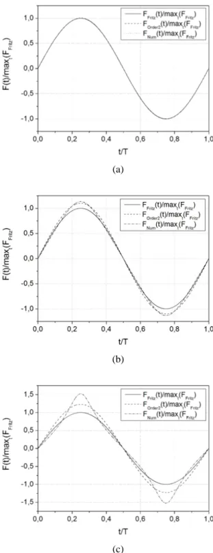
In order to compare the results issued from numerical simu-lations with the simple models developped in this paper, a sinu-soidal motion of period T is imposed on the inner cylinder. Since the fluid is assumed inviscid, there is no history effect [4] and this motion can be considered without loss of generality. Three con-finements are investigated:α= 1.1,α= 1.5 andα= 2. For each confinement, nine cases are computed (fromξ= 0, 1 toξ= 0, 9) so as to investigate the influence of large displacements in regards to the radial clearance. For each case, the numerical results have been checked to be independent of mesh refinements.
The maximum integrated forces are compared to those pre-dicted by the Fritz model (which corresponds to the leading-order formula Eqn. (46)) and the second leading-order model (given in Eqn. (76)). The results are summarized in Fig. 2. As expected, the models are all the more valid asξis small, i.e. as the inner cylinder displacement is small compared to the radial clearance. Furthemore, at a givenξ, they are more accurate for small values ofα. It is also an expected result since the perturbation param-eter ε= e(t)/R1which have been used to construct the models is all the smaller asαtends to unity. Of course, this argument is only true as long as the inviscid hypothesis holds, i.e. as long as the distance between the boundary layers of the inner and outer cylinder is large enough pν/ω<< R2− R1and more specifi-callyωR21(α− 1)2/ν>> 1 [6]. These figures also show that the
second order model gives better prediction than the Fritz one. The differences between the numerical code and the second
or-(a)
(b)
Figure 2. COMPARISONS BETWEEN THE MAXIMUM FORCES FOUND BY NUMERICAL SIMULATIONS WITH THE FRITZ MODEL (a) AND WITH THE SECOND ORDER MODEL (b).
der model are all under 3% untilξ= 0.6 whereas they are at more than 11% for the Fritz model at the sameξ. For the highest
ξachieved in this paper (ξ= 0.9), the differences are less than
25% for the second order model, whereas they are more than 40% for the Fritz model.
In order to gain some insight into the integrated fluid forces, it is fruitful to display their time history on a whole period. We will specialy consider the caseα= 2 for illustration but the same
phenomena occur forα= 1.5 andα= 1.1. The results for
differ-entξ(0.1, 0.6 and 0.9) are shown in Fig. 3. For small amplitudes of the inner cylinder (ξ= 0.1), the fluid forces predicted by the
Fritz model, the second order model and the numerical simula-tion are the same at each time (see Fig. 3(a)). Increasingξ, both the second order model and the numerical simulation predict big-ger maximum forces than the Fritz model, as it was already
men-(a)
(b)
(c)
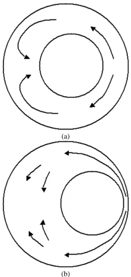
Figure 3. DIMENSIONLESS TIME HISTORY FLUID FORCES FORα= 2 IN CASESξ= 0.1 (a),ξ= 0.6 (b) andξ= 0.9 (c).
tioned. However a net difference can be seen: the second or-der model is for each time bigger than the Fritz model, whereas numerical simulations predict smaller forces during parts of the oscillation. Furthemore the time history contains two inflection points in each semi-period ]0, T /2[, ]T /2, T [, which are not pre-dicted by neither the Fritz model nor the second order one. This behaviour is all the more pronounced asξtends to 1 (as shown in Fig. 3(b)(c)) and has been already described in [15]. The follow-ing physical interpretation is proposed. Once the inner cylinder is subjected to an imposed motion, the fluid in front of it is sent back and a significant part finally push it (see Fig. 4(a)). The re-sulting force is then lower (see Fig. 3(c) at t ≈ 0, 12) that the one obtained with the Fritz and second order models, which are not able to reproduce properly this coupled advection/geometrical deformation effect. When the inner cylinder approaches more closely the outer one, this phenomenon is relaxed since the fluid amount sent back is lower and distributed on a larger area (see Fig. 4(b)). Moreover, the fluid particules in the squeeze film are all the more accelerated as the cylinders are closed, which results in a force increase (see Fig. 3(c) at t ≈ 0, 25) as in the case of a body falling to a wall [16, 17].
Conclusions
Extensions of the Fritz model are performed by taking ad-vection terms and the geometrical deformations induced by the inner circular cylinder movement into account. Approximated analytical solutions are found with a regular expansion per-formed until the second order on boundary-perturbation problem. At the leading-order, the advection term influences the local pres-sure on the moving inner cylinder, but not the integrated force, which can help to explain why the Fritz model, which consists in a pure added mass term, is accurate for small amplitude motions. At the first order, the advection term influences the fluid force and no term in the form (e(t)/R1) ¨e(t) is found. At the second order the geometrical deformation gives rise to a non linear modifica-tion of the added mass and no term in the form (e2(t)/R21) ˙e2(t) appears. The resulting fluid forces are then compared to numer-ical simulation predictions performed with a code able to take into account moving fluid domains. The second order model is shown to be more efficient than the Fritz model, specialy for high geometrical deformation. Nevertheless these two models are not able to reproduce strongly non linear potential effects found with the numerical simulations for high inner cylinder displacements. Forξlower than 0, 6, the differences between the Fritz and sec-ond order models are well below the incertainties on the input data in impulsive load analysis and these models are sufficient to have an idea about the forces level. However for higher ξ, these effects could influence the dynamical behaviour in fluid-structure interaction problems, and could prevent engineers from performing accurate prediction in case of shock or seismic load-ing. Hence further investigations need to be done so as to make this phenomenon more understandable. Moreover, future
exten-(a)
(b)
Figure 4. COUPLED ADVECTION/GEOMETRICAL DEFOR-MATION EFFECTS FOR SMALL (a) AND HIGH (b) AMPLI-TUDE MOTIONS
sions of the presented work would include viscous effects in or-der to characterize the damping term in the fluid forces.
REFERENCES
[1] Fritz, R., 1972. “The effects of liquids on the dynamics motion of immersed solids”. Trans. ASME, J. Eng. Ind., pp. 163–171.
[2] Leblond, C., Sigrist, J.-F., Laine, C., Auvity, B., and Peer-hossaini, H., 2006. “A review of fluid forces induced by a circular cylinder oscillating at low amplitude and high fre-quency in cylindrical confinement”. In ASME, Pressure Vessel and Piping Conference, PVP2006-ICPVT-11, Van-couver.
[3] Landau, L., and Lifschitz, E., 1959. Fluid Mechanics. Perg-amon Press, Oxford.
l’Ecole Polytechnique.
[5] Schlichting, H., 1979. Boundary Layer Theory, 7thEdition. McGraw-Hill.
[6] Axisa, F., 2001. Mod´elisation des syst`emes m´ecaniques.
Interactions fluide/structure. Herm`es.
[7] Lu, Y., and Rogers, R., 1995. “Instantaneous squeeze film force between a heat exchanger tube with arbitrary tube mo-tion and a support plate”. J. Fluids Struct., 9, pp. 835–860. [8] Zhou, T., and Rogers, R., 1997. “Simulation of two-dimensional squeeze film and solid contact forces acting on a heat exchanger tube”. J. Sound. Vib., 203, pp. 621–639. [9] Dyke, M. V., 1964. Perturbation Methods in Fluid
Mechan-ics. Academic Press, New York and London.
[10] Star-CD, 2004. Methodology, User Guide. CD Adapco. [11] Batchelor, G. K., 1997. An Introduction to Fluid Dynamics.
Cambridge University Press, Cambridge.
[12] Warsi, Z., 1980. “Conservation form of the navier-stokes equations in general non steady coordinates.”. AIAA
Jour-nal., 19, pp. 240–242.
[13] Sarrate, J., Huerta, A., and Donea, J., 1998. Arbitrary
La-grangian Eulerian Formulation for Fluid Multi-Rigid Bod-ies Interaction Problems. Computational Mechanics, New
trends and Application.
[14] Issa, R., 1985. “Solution of the implicitly discretised fluid flow equation by operator splitting.”. J. Comput. Phys., 62, pp. 40–65.
[15] Sigrist, J.-F., Laine, C., Lemoine, D., and Peseux, B., 2003. “Choice and limits of a linear fluid model for the numeri-cal study in dynamic fluid structure interaction problem”. In Proceedings of ASME, Vol. 454 of Pressure Vessel and
Piping, Cleveland, pp. 87–93.
[16] Wang, Q. X., 2004. “Interaction of two circular cylinders in inviscid fluid.”. Phys. Fluids., 16, pp. 4412–4425. [17] Joseph, G. G., Zenit, R., Hunt, M. L., and Rosenwinkel,
A. M., 2001. “Particle-wall collisions in a viscous fluid”. J.
Fluid Mech., 433, pp. 329–346.