Aerial Co-Manipulation with Cables: The Role of Internal Force for Equilibria, Stability, and Passivity

(1)

HAL Id: hal-01551105

https://hal.laas.fr/hal-01551105v3

Submitted on 11 Feb 2018

HAL is a multi-disciplinary open access

archive for the deposit and dissemination of

sci-entific research documents, whether they are

pub-lished or not. The documents may come from

teaching and research institutions in France or

abroad, or from public or private research centers.

L’archive ouverte pluridisciplinaire HAL, est

destinée au dépôt et à la diffusion de documents

scientifiques de niveau recherche, publiés ou non,

émanant des établissements d’enseignement et de

recherche français ou étrangers, des laboratoires

publics ou privés.

Aerial Co-Manipulation with Cables: The Role of

Internal Force for Equilibria, Stability, and Passivity

Marco Tognon, Chiara Gabellieri, Lucia Pallottino, Antonio Franchi

To cite this version:

Marco Tognon, Chiara Gabellieri, Lucia Pallottino, Antonio Franchi. Aerial Co-Manipulation with

Cables: The Role of Internal Force for Equilibria, Stability, and Passivity. IEEE Robotics and

Au-tomation Letters, IEEE 2018, 3 (3), pp.2577 - 2583. �10.1109/LRA.2018.2803811�. �hal-01551105v3�

(2)

Preprint version, final version at http://ieeexplore.ieee.org/ IEEE Robotics and Automation Letters 2018

Aerial Co-Manipulation with Cables: The Role of Internal Force for

Equilibria, Stability, and Passivity

Marco Tognon

1

_{, Chiara Gabellieri}

1,2,†

_{, Lucia Pallottino}

2

_{, and Antonio Franchi}

1

Abstract— This paper considers the cooperative manipulation of a cable-suspended load with two generic aerial robots without the need of explicit communication. The role of the internal force for the asymptotic stability of the beam position-and-attitude equilibria is analyzed in depth. Using a nonlinear Lyapunov-based approach, we prove that if a non-zero inter-nal force is chosen, then the asymptotic stabilization of any desired beam attitude can be achieved with a decentralized and communication-less master-slave admittance controller. If, conversely, a zero internal force is chosen, as done in the majority of the state-of-the-art algorithms, the attitude of the beam is not controllable without communication. Furthermore, we formally proof the output-strictly passivity of the system with respect to an energy-like storage function and a certain input-output pair. This proves the stability and the robustness of the method during motion and in non-ideal conditions. The theoretical findings are validated through extensive simulations.

I. INTRODUCTION

Over the last decade UAVs (Unmanned Aerial Vehicles) have risen the interest of a larger and larger audience for their wide application domain. Recently, aerial physical interaction, using aerial manipulators [1], [2] or exploiting physical links as cables [3], has become a very popular topic. One interesting and applicative problem is the aerial manipu-lation of large objects, for which cooperative approaches are usually applied because they allow to overcome the limited payload of a single platform, thus lifting larger and heavier loads [4].

Many works targeted this problem proposing different methods and solutions. In [5], [6] cooperative aerial trans-portation of a rigid and an elastic object is considered, re-spectively. In [7] the use of multiple flying arms is exploited to address the problem. Aerial manipulation via cables is another interesting solution to the problem since it can reduce the couplings between the load and the robot attitude dynamics. Examples of cooperative aerial manipulation using cables are studied in [8]–[10]. All these examples rely on a centralized control. Instead, a decentralized algorithm, as in [11], is more robust and scalable with respect to (w.r.t.) the number of robots.

†_{The first two authors have equally collaborated to the manuscript, and}

can both be considered as first author.

1_LAAS-CNRS, _Universit´e _de _Toulouse, _CNRS, _Toulouse,

France, antonio.franchi@laas.fr, marco.tognon@laas.fr, cgabellieri@laas.fr

2_{Centro di ricerca E. Piaggio, Universit`a di Pisa, Largo Lucio Lazzarino}

1, 56122,Pisa, Italylucia.pallottino@unipi.it

This work has been funded by the European Union’s Horizon 2020 research and innovation program under grant agreement No 644271 AEROARMS. FW f1= t1n1 f2= t2n2 A1 FL B1 A2 B2 f1 _f2 b1 b2 FR1 _F R2 OL tLrL tLrL xL zL

Fig. 1: Representation of the system and its major variables. The two aerial vehicles do not need to be necessarily quadrotors since the analysis and control design is valid for general aerial vehicles.

However, the major bottleneck in decentralized algorithms is the explicit communication. Communication delays and packet losses can affect the performance and even the sta-bility of the systems. Limiting the need for explicit com-munication allows to reduce the complexity as well. In [12] the authors proposed one of the first decentralized leader-follower algorithm without explicit communication, for ob-jects transportation performed by mobile ground robots. Aerial cooperative transportation by two robots without explicit communication has been addressed also in [13] for a cable-suspended beam-like load, and a leader-follower paradigm has been proposed. Here the leader follows an external position reference, while the horizontal position of the follower is controlled with an admittance filter, trying to keep the cable always vertical (zero internal force). A similar approach has been proposed in [14] but relying on a visual feedback. However, those methods do not deal with the load pose control and do not provide a formal stability proof.

For the same system composed by two aerial robots carrying a cable suspended beam-like load (see Fig. 1 for a schematic representation), we propose a decentralized algo-rithm relying only on implicit communication. Our algoalgo-rithm uses a master-slave architecture with an admittance filter on both robots (not only on the slave as in the related state of the art), to make the overall system compliant/robust to external disturbances.

One of our main contributions is the constructive and intuitive method to choose the controller input to stabilize the load at a desired pose. The control of both position and orientation turns the simpler transportation task found in the state of the art in a full-manipulation one.

We show that those inputs are parametrized by the internal force of the load that plays a crucial role in the equilibria stability. Differently from the state of the art algorithms, which are not formally guaranteed to converge, we also provide a formal proof of the stability through Lyapunov’s

(3)

direct method. Furthermore, we prove that the controlled system is output-strictly passive w.r.t. a relevant input-output pair. This provides a bound for the energy variations during the manipulation and an index of robustness of the method. In Sec. II we derive the model. In Sec. III we present the control strategy and the equilibria of the system. Their stability is discussed in Sec. IV. In Sec. V we prove the passivity and stability of transportation. Simulation results and conclusive discussions are presented in Sec. VI and VII, respectively.

II. SYSTEMMODELING

The considered system and its major variables are shown in Fig. 1. The beam-like load is modeled as a rigid body with

mass mL2 R>0 and a positive definite inertia matrix JL2

R3⇥3_{. We define the frame F}_L₌_{O_L_{, x}_L_{, y}_L_{, z}_L_{} rigidly}

attached to it, where OLis the the load center of mass (CoM).

Then, we define an inertial frame FW ={OW, xW, yW, zW}

with zW oriented in the opposite direction to the gravity

vector. The configuration of the load is then described by the

position of OL and orientation of FL with respect to FW,

i.e., by the vector pL2 R3 and the rotation matrix RL2

SO(3), respectively. Its dynamics is given by the Newton-Euler equations

mL¨pL= mLge3+ fe

˙

RL= S(!L)RL

JL˙!L= S(!L)JL!L+ ⌧e !>LBL!L,

where, !L 2 R3 is the angular velocity of FL w.r.t. FW

expressed in FL, S(?) is the operator such that S(x)y =

x_{⇥y, g is the gravitational constant, e}iis the canonical unit

vector with a 1 in the i-th entry, feand ⌧e2 R3are the sum of

external forces and moments acting on the load, respectively.

The positive definite matrix BL2 R3⇥3 is a damping factor

modeling the energy dissipation phenomena.

The load is transported by two aerial robots by means

of two cables, one for each robot. We denote with Ai the

attachment point of the i-th cable to the i-th robot, with i = 1,2, and we define the frame FRi={Ai, xRi, yRi, zRi}

rigidly attached to the robot and centered in the attachment point. The i-th robot configuration is described by the

po-sition of Ai and orientation of FRi w.r.t. FW, denoted by

the vector pRi2 R3, and the rotation matrix RRi2 SO(3),

respectively. We assume that a position controller is applied

to the aerial robot, able to track any C2 _{trajectory with}

negligible error in the domain of interest, independently from external disturbances. Indeed, with the recent robust controllers (as the one in [15] for both unidirectional- and multidirectional-thrust vehicles) and disturbance observers for aerial vehicles, one can obtain very precise motions, even in the presence of external disturbances. However, the proposed control method results particularly robust to non-ideality, thanks to its passivity nature (see Sec. V). As a consequence, in real applications, a precise tracking is actually not needed for the stability, but only to achieve perfect performance.

The closed loop translational dynamics of the robot subject to the position controller is then assumed as the one of a

double integrator: ¨pRi= uRi, where uRi is a virtual input

to be designed. If we consider a multidirectional-thrust platform capable of controlling both position and orientation independently [16], the double integrator is an exact model of the closed loop system apart from modeling errors. In the case of underactuated unidirectional-thrust vehicle, the double integrator is instead a very good approximation. Indeed the rotational dynamics is totally decoupled from the translational one and it is much faster than the latter, allowing to apply the time-scale separation principle. At this stage it might seem that the platform is ‘infinitely stiff’ w.r.t. the force produced by the cable. However, we shall re-introduce

a compliant behavior by suitably designing the input uRi.

The other end of the i-th cable is attached to the load

at the anchoring point Bi described by the vector Lbi2 R3

denoting its position with respect to FL. The position of Bi

w.r.t. FW is then given by bi= pL+ RLLbi. To simplify

the discussion we assume, without loss of generality, that

L_b

1= [kLb1k 0 0]>.

Assumption 1. The two anchoring points are placed such that

the load CoM coincides with their middle point, i.e.,Lb1=

L_b

2. This assumption is rather easy to meet in practice.

We model the i-th cable as a unilateral spring along its principal direction, characterized by a constant elastic coefficient ki2 R>0, a constant nominal length denoted by l0i

and a negligible mass and inertia w.r.t. the ones of the robots and of the load. The attitude of the cable is described by the normalized vector, ni= li/klik, where li= pRi bi. Given

a certain elongation klik of the cable, the latter produces a

force acting on the load at Bi equal to:

fi=tini, ti=

(

ki(klik l0i) if klik l0i>0

0 otherwise . (1)

ti2 R 0denotes the tension along the cable and it is given

by the simplified Hooke’s law. As usually done in the related literature, we assume that the controller and the gravity force always maintain the cables taut, at least in the domain of interest. The force produced at the other hand of the cable, namely on the i-th robot at Ai, is equal to fi.

Considering the forces that robots and load exchange by means of the cables, the dynamics of the full system is:

˙vR= uR

˙vL= ML1( cL(vL) gL+ G(qL)f) , (2)

where qR= [p>R1 p>R2]>, qL= (pL, RL), vR= [˙p>R1 ˙p>R2]>,

vL = [˙p>L !L>]>, uR= [uR1> u>R2]>, f = [f1> f2>]> where

fi is given in (1), and is a function of the state, ML=

diag(mLI3, JL) and I3 2 R3⇥3 the identity matrix, gL =

[ mLge>3 0]>, cL= [0 S(!L)JL!L !>LBL!L]> and

G = 

I3 I3

S(Lb1)R>L S(Lb2)R>L .

We remark that the two dynamics in (2) are coupled together by the cable forces in (1).

(4)

Load Cable 1 Cable 2 Robot 1 Robot 2 Admittance 1 Admittance 2 f1 b1 f2 b2 f1 f2 pR2 pR1 uR2 uR1 pR1, ˙pR1 pR2, ˙pR2 ⇡A2 ⇡A1

Fig. 2: Schematic representation of the overall system including both physical and control blocks.

Control problem

In this work we aim to: i) stabilize the load at a desired configuration, ¯qL= (¯pL, ¯RL); ii) preserve the stability of the

load during its transportation.

Assuming a perfect knowledge of the system dynamic model, and a perfect state estimation, one could use a centralized control approach, as in [8], [9]. We are instead interested in solving the mentioned objectives using a decen-tralized approach without explicit communication between the robots.

III. CONTROLDESIGN ANDEQUILIBRIA

To achieve the previous control objectives we propose the use of an admittance filter for both robots, i.e., setting:

uRi= MAi1( BAi˙pRi KAipRi fi+ ⇡Ai) , (3)

where the tree positive definite symmetric matrices MAi, BAi, KAi2 R3⇥3are the virtual inertia of the robot, the

virtual damping, and the stiffness of a virtual spring attached

to the robot, and ⇡Ai2 R3 is an additional input (see Fig. 2

for a schematic representation). Notice that (3) does not require explicit communication. Indeed it requires only local information, i.e., the state of the robot (pRi, ˙pRi), and the

force applied by the cable fi. The first can be retrieved with

standard on-board sensors, while the second can be directly measured by an on-board force sensor or estimated by a sufficiently precise model-based observer as done in [13], [16].

Combining equations (2) and (3) we can write the closed

loop system dynamics as ˙v = m(q,v,⇡A)where

m(q,v,⇡A) =



M_A1( BA˙pR KApR f + ⇡A)

M_L1( cL(vL) gL+ Gf) , (4)

with q = (qR, qL), v = [v>R v>L]>and ⇡A= [⇡A1> ⇡A2>]>.

Fur-thermore MA=diag(MA1, MA2), BA=diag(BA1, BA2)and

KA=diag(KA1, KA2). In order to coordinate the motions of

the robots in a decentralized way we propose a master-slave approach. Only one robot, namely the designated master, will have an active control of the system. Choosing robot 1 as

master and robot 2 as slave we set KA16= 0, KA2= 0.

We say that q is an equilibrium configuration if 9 ⇡A s.t.

0 =m(q,0,⇡A),i.e, if the corresponding zero-velocity state

(q, 0)is a forced equilibrium for the system (4) for a certain

forcing input ⇡A. We say that an equilibrium configuration q

is stable, unstable, or asymptotically stable if (q,0) is stable, unstable, or asymptotically stable, respectively.

Configuration Space Parameter Space

⇧A( ¯qL) S tL<0 Q (tL, ¯qL) S tL>0 Q+_(t L, ¯qL) tL< 0 tL> 0 tL= 0 ¯ qL Load qL= (pL, RL) ⇡A q = (pR1, pR2, pL, RL) Constant Input Q(0, ¯qL) ¯ qL

Configuration SpaceFull System

R3_{⇥ SO(3)}

R6 _R9_{⇥ SO(3)}

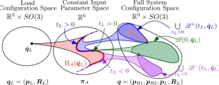
Fig. 3: Relation between the equilibria and forcing control input. In particular, starting from the left: to a desired load configuration of

equilibrium it corresponds a forcing input in the subsetPA(¯qL)of

dimension one (inverse problem). Then, moving to the right: to a

forcing input inPA(¯qL)it corresponds an equilibrium in the subsets

Q+(tL,¯qL), Q (tL,¯qL) or Q(0, ¯qL) according to the value of tL

(direct problem). The orange line inside Q+_(t

L,¯qL)corresponds to

the equilibria q 2 Q+_(t

L,¯qL)such that qL= ¯qL.

In the following we shall prove that for any desired load configuration ¯qL there exists a set PA(¯qL)⇢ R6 such that

for any ⇡A2 PA(¯qL)one can compute a ¯qR, depending on

¯qLand ⇡A, that makes ¯q = ( ¯qL,¯qR)an asymptotically stable

equilibrium with ⇡A as forcing input. As we shall see, a

key role in all the following analyses is played by the load internal force, defined as

tL:=1₂f>⇥I3 I3⇤>RLe1=: 1₂f>rL, (5)

where rL =⇥I3 I3⇤>R¯Le1. We have that if tL>0 the

internal force is a tension (the work of the internal force is positive if the distance between the anchoring points increases) while if tL<0 the internal force is a compression

(viceversa, the work is positive if the distance decreases). A. Equilibrium Configurations of the Closed Loop System

We firstly carefully analyze the relation between equilib-rium configurations, from now on simply called equilibria,

and the forcing input ⇡A. In particular, we shall study:

i) equilibria inverse problem: which is the set of inputs (and

corresponding robot positions) that equilibrates a desired ¯qL

(Theorem 1); ii) equilibria direct problem: which is the set of equilibria if ⇡A, chosen in the aforementioned set, is applied

to the system (Theorem 2). A schematic representation of the results described in the theorems is given in Fig. 3. Theorem 1 (equilibria inverse problem). Consider the closed loop system (4) and assume that the load is at a given desired configuration qL= ¯qL= (¯pL, ¯RL). For each internal force

tL2 R, there exists an unique constant value for the forcing

input ⇡A= ¯⇡A(and an unique position of the robots qR= ¯qR)

such that ¯q = ( ¯qL,¯qR)is an equilibrium of the system.

In particular ¯⇡A and ¯qR= [¯p>R1 ¯p>R2]> are given by

¯⇡A(¯qL,tL) = KA¯qR+ ¯f (¯qL,tL) (6) ¯pRi(¯qL,tL) = ¯pL+ ¯RLLbi+ ✓ k ¯fik ki +l0i ◆ ¯fi k ¯fik, (7) for i = 1,2, where ¯ f (¯qL,tL) =  ¯_f₁ ¯ f2 = mLg 2  I3 I3 e3+tL  I3 I3 R¯Le1. (8)

(5)

Proof. The desired load configuration ¯qL can be equilibrated

if there exists at least a ¯qR and a ⇡Asuch that:

m( ¯q,0,⇡A) = 0. (9)

Consider the last six rows of (9). We must find the f solving

Gf = gL. (10)

Gis not invertible since rank(G) = 5, thus we have to verify

that a solution for (10) exists. Expanding (10) we obtain

f1+ f2= mLge3 (11)

S(Lb1) ¯R>Lf1+ S(Lb2) ¯RL>f2= 0. (12)

Then, substituting in (12) the f1 obtained from (11) we

have 2S(L_b

1) ¯R>Lf2= S(Lb1) ¯RL>mLge3, for which f2=

mLge3/2 is always a solution. Therefore, all the solutions

of (10) can be written as ¯

f = G†gL+ rLtL, (13)

where G†₌_1/2[I₃_I₃_]>_{is the pseudo inverse of G, r}_L_{2 R}6

is a vector in Null(G) , and tL2 R is an arbitrary number.

We computed rL= [f1>f2>]>from (11) and (12) imposing

the right hand side equal to zero. From (11) f2= f1, and

replacing it into (12) we obtain S(2Lb1) ¯R>Lf1= 0 which

is verified if f1=tLR¯Le1 with tL2 R. Finally we obtain

rL=⇥I3 I3⇤>R¯Le1, as in the definition (5).

Equation (13) can be then rewritten as (8). The expression

of ¯pRiin (7) is computed using (1) and the kinematics of the

system. Notice that (7) is singular when ¯fi= 0for some i.

However this can always be avoided properly choosing tL.

Lastly, from the first six rows of (9) we have that ¯qL is

equilibrated if ⇡A= ¯⇡A, where ¯⇡Ais defined as in (6).

Remark 1. Based on Theorem 1 we can define a set PA(¯qL) ={⇡A2 R6: ⇡A=¯⇡A(¯qL,tL) for tL2 R} which has

dimension 1, since it is parametrized by the scalar tL2 R.

Remark 2. Given a desired load configuration ¯qL to

equili-brate, Theorem 1 and its constructive proofs, give an intuitive

method for choosing the forcing input ⇡A. In particular one

has to choose only the value of the internal force tL.

Once tL is chosen and the input ⇡A= ¯⇡A(tL,¯qL)is applied

to the system, it is not in general granted that ( ¯qL,¯qR)is the

only equilibrium of (4), i.e., the equilibria direct problem may have multiple solutions.

Theorem 2 (equilibria direct problem). Given tL2 R and

the corresponding ¯⇡A 2 PA(¯qL) computed as in (6), the

equilibria of the system (4), when the input ⇡A=¯⇡A(tL,¯qL)is

applied, are all and only the ones described by the following conditions tLRLe1⇥ ¯RLe1= 0 pR1= ¯pR1 pL= pR1 RLLb1 ✓ k ¯f1k k1 +l01 ◆ ¯f1 k ¯f1k = = ¯pL+ ( ¯RL RL)Lb1 pR2= pL+ RLLb2+ ✓ k ¯f2k k2 +l02 ◆ ¯f2 k ¯f2k. (14) A1 FL B1 A2 B2 f1 f2 b1 b2 B1 A2 f2 FL b1 b2 A1 f1 B2

(a) Two equilibria for tL 6= 0.

On the top and on the bottom one equilibrium configuration in Q+_(t_L_,_¯q_L₎ _{and Q (t}_L_,_¯q_L_), re-spectively. A2 A2 A2 A2 A2 FL B2 A1 B1 b2 b1

(b) Five of the possible infinite equilibria in Q(0, ¯qL). In vivid

color the configuration ¯q. The fi-nal load pose depends on the ini-tial conditions.

Fig. 4: 2D representation of the equilibria varying tL.

Q(tL,¯qL)denotes the set of configurations respecting (14).

Proof. Given tL2 R, and ¯⇡A2 PA(¯qL), a configuration q

is an equilibrium if m(q,0, ¯⇡A) = 0. The first six rows are

KAqR+ f ¯⇡A= 0. Then, from (6) we have that

f = KA(¯qR qR) + ¯f . (15)

Multiplying both sides of (15) by G and using (10) we obtain

GKA(¯qR qR) + G ¯f = gL. Then, using KA2= 0, and the

expression of ¯f in (8), we get  _K A1eR1 S(Lb₁)RLK_A1e_R1 +  _m Lge3 2S(L_b 2)R>LR¯Le₁tL =  mLge3 0 , (16)

where eRi= (¯pRi pRi). The top row of (16) implies that

eR1= 0, hence pR1= ¯pR1. Replacing eR1= 0in the bottom

part of (16) we obtain

S(Lb2)R>LR¯Le1tL= 0, Lb2⇥ R>LR¯Le1tL= 0

, RLe1⇥ ¯RLe1tL= 0. (17)

We can retrieve pL and pR2, using (1) and the kinematics.

Remark 3. If tL=0 the conditions in (17) hold for all the

possible load attitudes RL2 SO(3). This means that Q(0, ¯qL)

contains all the RL2 SO(3) and the qR, pL computed from

RLusing (14). Figure 4b illustrates some of these equilibria.

For tL 6= 0, it is required that RLe1 is parallel to

¯

RLe1. This can be obtained with RL = RL(k,f) =

¯

RLRz_L(kp)Rx_L(f), where k = 0,1, f 2 [0,2p], and Rz_L(·)

and Rx_L(·) are the rotations about zL and xL,

respec-tively. Considering that Lb1 is parallel to xL we have that

Rz_L(kp)Rx_L(f)Lb1is either equal toLb1if k = 0 or to Lb1

if k = 1. Therefore, using (14), we obtain either pL= ¯pL if

k = 0 or pL= ¯pL+2b1if k = 1. Fig. 4a provides a simplified

representations of the two different sets of equilibria for k = 0 and k = 1, formally defined as follows:

• Q+(tL,¯qL) ={q 2 Q(tL,¯qL)|RL= RL(0,f)8f}, • Q (tL,¯qL) ={q 2 Q(tL,¯qL)|RL= RL(1,f)8f}.

Notice that Q(0, ¯qL) is parametrized by an element in

SO(3) (any RL2 SO(3) is allowed), while Q+(tL,¯qL)and

Q (tL,¯qL), for tL6= 0, are parametrized by an element in

(6)

SO(1) (RL(0,f) and RL(1,f), for any f 2 [0,2p],

respec-tively). For all tL, the load rotation about xL is arbitrary

because the robots can not apply any torque along xL, so

the corresponding rotation results uncontrollable.

We can conclude that choosing tL=0 (equilibrium with

vertical cables) every orientation of the load is contained in the equilibrium set and the load equilibrium positions are

free to move on a sphere of radius kL_b

1k centered on B1.

Contrarily, tL6= 0 is a much better choice. In this case, a

part from the rotation about the xL axis, there are only two

distinct equilibria, and one is exactly qL= ¯qL, as expected.

For the other one the load orientation is parallel to the one in ¯qL but its position is reflected w.r.t. B1(see Fig. 4a for an

example).

IV. STABILITY OF THEEQUILIBRIA

In this section we shall analyze the stability of the equi-libria discovered in Sec. III-A. Firstly we define x = (q,v) as the state of the system, ¯x = ( ¯q,0) the desired equilibrium state, and the following sets (subspaces of the state space):

• X (tL,¯qL) ={x : q 2 Q(tL, ¯qL), v = 0}, • X (0, ¯qL) ={x : q 2 Q(0, ¯qL), v = 0}, • X+(tL,¯qL) ={x : q 2 Q+(tL,¯qL), v = 0}, • X (tL,¯qL) ={x : q 2 Q (tL,¯qL), v = 0}.

Theorem 3. Let us consider a desired load configuration

¯qL. For the system (4) let the constant forcing input ⇡A be

chosen in PA(¯qL)corresponding to a certain internal force

tL. Then x belonging to:

• X+(tL,¯qL)is locally asymptotically stable if tL>0; • X (tL,¯qL)is unstable if tL>0;

• X (0, ¯qL)is locally asymptotically stable; • X+(tL,¯qL)is unstable if tL<0;

• X (tL,¯qL)is locally asymptotically stable if tL<0.

Proof. Let us consider the following Lyapunov candidate:

V (x) =1

2(v>RMAvR+ e>RKAeR+ v>LMLvL+ +k1(kl1k l01)2+k2(kl2k l02)2) l>1f¯1+

l₂>f¯2+tL(1 ( ¯RLe1)>RLe1) +V0,

(18)

where V02 R 0and eR= ¯pR1 pR1. For an opportune choice

of V0, V (x) is a positive definite, continuously differentiable

function in the domain of interest for which we have that

xmin =argminxV (x) is such that xmin 2 X (0, ¯qL) and

xmin2 X+(tL,¯qL)for tL>0. The complete proof is provided

in technical report in the multimedia materials. In particular,

if tL 0, we can choose the term V0such that V (x) 0 and

V ( ¯x) = 0. Notice that V (x) = 0 for all x 2 X (0, ¯qL) and

x_{2 X}+_(t_L_,_¯q_L₎_{for t}_L_>_0.

Computing the time derivative of (18) and replacing (4), (1) and (8) we obtain ˙V = vR>BAvR !L>BL!L that

is clearly negative semidefinite. In particular ˙V (x) = 0 for

all x 2 E {x : vR= 0, !L= 0}

Since ˙V is only negative semidefinite, to prove the asymp-totic stability we rely on the LaSalle’s invariance

princi-ple [17]. Let us define a positively invariant set Wa =_{{x :}

V (x)  a with a 2 R>0}. By construction Wa is compact

since (18) is radially unbounded andW0 is compact (W0=

X (0, ¯qL) and W0= X+(tL,¯qL) for tL =0 and tL >0,

respectively, are both compact sets). Then we need to find

the largest invariant set M in E = {x 2 Wa | ˙V (x) = 0}.

A trajectory x(t) belongs identically to E if ˙V (x(t)) ⌘

0 , vR(t) ⌘ 0 and !L(t) ⌘ 0 , m(q(t),0,⇡A) = 0 for all

t 2 R>0. Therefore x has to be an equilibrium, and from

Theorem 2 we have that ˙V (x(t)) ⌘ 0 , x(t) 2 X (tL,¯qL).

Thus we obtain M = Wa\ X (tL,¯qL).

For tL >0, it is easy to see that for a sufficiently

small a, X+_(t_L_,_¯q_L₎_{✓ W}_a _{but X (t}_L_,_¯q_L₎_{\ W}_a ₌_{?. This}

because V (x) = 0 for x 2 X+_(t_L_,_¯q_L_{), while V (x) > 0}

for x 2 X (tL,¯qL). Indeed, in (18), for x 2 X (tL,¯qL),

the term tL(1 ( ¯RLe1)>RLe1) =2tL>0. Therefore M =

X+(tL,¯qL). All conditions of LaSalle’s principle are

satis-fied and X+_(t

L,¯qL)is locally asymptotically stable.

On the other hand, for tL=0 we have that X (tL,¯qL)✓ Wa

for every sufficiently small a. Therefore M = X (tL,¯qL)

and, as before, we can conclude that X (tL,¯qL) is locally

asymptotically stable for the LaSalle’s invariance principle. Now, let us investigate the stability for tL<0. As before,

with an opportune choice of V0, we have that V (x) = 0

for x 2 X+_(t

L,¯qL). However X+(tL,¯qL) is a set of

ac-cumulation for the points where V (x) < 0. Indeed, consider v = 0, pR1= ¯pR1, RL such that ( ¯RLe1)>RLe1=1 e, with

e > 0 arbitrarily small, pL and pR2 as in (14). Under this

conditions, we have that V (x) = tL(1 ( ¯RLe1)>RLe1) =

tLe < 0. Then, ˙V(x) < 0 in a neighborhood of X+(tL,¯qL).

All conditions of Chetaev’s theorem [17] are satisfied, and we can conclude that X+_(t_L_,_¯q_L₎_{is an unstable set.}

Finally, to study the stability of X (tL,¯qL) for tL6= 0,

let us consider a desired load configuration ¯q0

L= (¯p0L, ¯R0L)

such that ¯p0

L= p0L+2 ¯RLe1 and ¯R0L= RL(1,f) for a

cer-tain f. Then we choose ⇡0

A2 PA(¯qL0) with tL0 = tL. For

the reasoning in Sec. III-A, we have that X+_(t0

L,¯q0L) =

X (tL,¯qL). Furthermore, for the previous results, if tL>0,

t0

L<0 and X+(tL0, ¯qL0)is unstable. Therefore, X (tL,¯qL)is

unstable too. A similar reasoning can be done to prove that X (tL,¯qL)is locally asymptotically stable for tL<0.

V. PASSIVITY ANDSTABILITY OFMANIPULATION

Theorem 3 characterizes the stability of all the possible static equilibria given a certain constant forcing input. In particular, it shows that one has to choose tL>0 and ⇡A2

PA(¯qL)to let the system asymptotically converge to a desired

load configuration. On the contrary, one must avoid tL=0

because the control of the load attitude and its position is not possible. Notice that this last case is the most used in the literature, where the attempt is made to keep the cables always vertical, i.e., with no internal forces.

Let us now show how one can exploit the input ⇡A1

in order to move the load between two distinct positions.

From (6)–(8) and from the fact that KA2= 0, it descends that

only ¯⇡A1, in ¯⇡A=[¯⇡>A1 ¯⇡>A2]>, actually depends on the desired

load position ¯pL. This makes robot 1 able to steer alone the

(7)

done by first plugging a new desired position ¯p0

L in (6) thus

computing a new ¯p0

R1, and then plugging ¯p0R1 in (7) in order

to compute the new constant forcing input ¯⇡0

A1. However,

one may want to minimize the transient phases generated by a piecewise constant forcing input. It is sufficient to design ⇡A1 as

⇡A1(t) = ¯⇡A1+ uA1(t), (19)

where uA1(t) is a smooth function such that ⇡A1(0) = ¯⇡A1

and ⇡A1(tf) = ¯⇡A10 for tf 2 R>0.

To ensure that the system remains stable when the input is time-varying, we shall prove that the system is output-strictly passive w.r.t. the input-output pair (u,y) = (uA, vR).

Theorem 4. If ⇡Ais defined as in (19) for a certain ¯q and

¯q0_{with t}_L _{0, then system (4) is output-strictly passive w.r.t.}

the storage function (18) and the input-output pair (u,y) = (uA, vR).

Proof. In the proof of Theorem 3 we already shown that (18) is a continuously differentiable positive definite function for

tL 0, properly choosing V0. Furthermore, replacing (19)

into (3), and differentiating (18) we obtain ˙V = vR>BAvR+ vR>uA !>LBL!L

u>y y>BAy = u>y y> (y), (20)

with y> _{(y) >}_{0 8 y 6= 0. Therefore, system (4) is}

output-strictly passive [17].

Thanks to the passivity of the system we can say that for a bounded input provided to the master, the energy of the system remains bounded too, and in particular it

stabilizes to a new constant value as soon as uA1 becomes

constant again. This means that while moving the master, the overall state of the system will remain bounded, and will converge to another specific equilibrium configuration when the master input becomes constant. Furthermore, it is well known that passivity is a robust property, especially w.r.t. model uncertainties. In particular, choosing ⇡A2 PA(¯qL)for

a given ¯q, the system remains asymptotically stable even in the presence of some parameter uncertainties, but it will converge to a ¯q0 _{that is slightly different from ¯q.}

Remark 4. Once the desired load pose is decided and the

value of tL is chosen, one can compute the control input

⇡Aand send it to the robots. Afterwards, if tL>0 the robots

will steer the load to the desired configuration preserving the stability and without the need of sending data to each other. The cooperative task is performed exploiting the implicit communication through the forces that the robots exchange and feel from the cables and the object.

VI. NUMERICALVALIDATION

In this section we shall describe the results of several numerical simulations validating the proposed method and all the presented theoretical concepts and results.

For the simulation we considered a quadrotor-like vehicle with its proper nonlinear dynamics together with a geometric position controller, even though, our method can be applied

to more general flying vehicles. System and control parame-ters are reported in Tab. I. Notice the smaller apparent inertia of the slave, chosen to make it more sensitive to external forces.

Let us consider the desired equilibrium ¯q = ( ¯pL, ¯RL),

whose value are in Tab. I, where ( ¯f, ¯q, ¯y) are the Euler

angles that parametrize ¯RL. We performed several

simula-tions with ⇡A2 PA(¯qL) computed as in (6) for the cases:

1) tL1=1.5 [N] > 0, 2) tL2=0 [N], 3) tL3= 1 [N] < 0.

To test the stability of the equilibria, we initialized the system in different initial configurations and we let it evolve. Figure 6 shows the position and orientation error for the three tLand several different initial conditions. 1) For tL=tL1, the

system always converges to a state belonging to X+_(t

L,¯qL),

independently from the initial state, validating the asymptotic stability of X+_(t

L,¯qL)when tL>0. 2) For tL2, the system

final state belongs to X (0, ¯qL). The particular final attitude

of the load depends on the initial state. 3) For tL3, the system

never converges to X+_(t_L_,_¯q_L₎_{even with a very close initial}

configuration. This is due to the instability of X+_(t_L_,_¯q_L₎

when tL<0. Fig. 5 shows the evolution of the system starting

from two different initial states for the three cases.

In another set of simulations, shown in detail in the

attached technical report, the master input ⇡A1(t) is chosen

as in (19) to bring the load in ¯p0

L= [4.5 4.5 5]>[m]. We

observed that, as expected, for both tL=tL1 and tL=tL2

the system remains stable during the master maneuver. Once the input becomes constant, the master stops and the system converges to ¯q for tL=tL1. For tL=tL2, the final load attitude

depends on the particular motion, and it is in general different from ¯q.

Additional simulations in non-ideal conditions are pro-vided in the attached technical report. The results show that thanks to the passivity of the system, the latter is very robust to the considered non-idealities. Some representative simulations are available in the attached video too.

VII. CONCLUSIONS

This work deals with the decentralized cooperative manip-ulation of a cable-suspended load performed by two aerial vehicles. The proposed master-slave architecture exploits an admittance controller in order to coordinate the robots with implicit communication only, exploiting the cable forces. The passivity of the system has been proven, and the stability of the static equilibria has been studied highlighting the crucial role of the internal force. In particular, contrarily from what

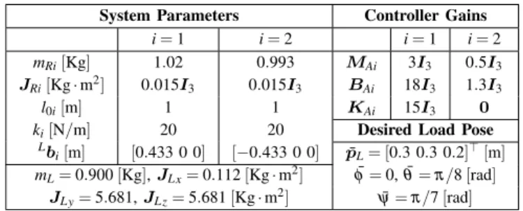
System Parameters Controller Gains i = 1 i = 2 i = 1 i = 2 mRi[Kg] 1.02 0.993 MAi 3I3 0.5I3

JRi[Kg · m2] 0.015I3 0.015I3 BAi 18I3 1.3I3

l0i[m] 1 1 KAi 15I3 0

ki[N/m] 20 20 Desired Load Pose L_b

i[m] [0.433 0 0] [ 0.433 0 0] ¯pL= [0.3 0.3 0.2]>[m]

mL=0.900 [Kg], JLx=0.112 [Kg · m2_] _{¯f = 0, ¯q = p/8 [rad]}

JLy=5.681, JLz=5.681 [Kg · m2_] _{y = p/7 [rad]}_¯

TABLE I: Parameters used in the simulations.

(8)

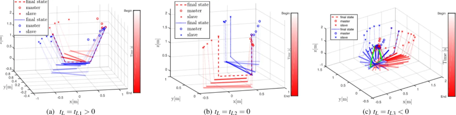
-0.5 0 0.5 0.8 1 1.5 0.6 2 0.4 0.2 0 -0.2 ₁ 0.5 -0.4 -1 -0.5 0 End Begin (a) tL=tL1>0 0 0.5 1 1 1.5 2 0.5 1 0.5 0 0 _-0.5 End Begin (b) tL=tL2=0 -1 1.5 1 0 2 y[m] 1.5 0.5 z[ m ] 1 x[m] 1 0 0.5 0 -0.5 -0.5 2 End Begin T im e [s ] final state master slave final state master slave (c) tL=tL3<0

Fig. 5: Each figure shows the evolution of the system from two different initial conditions (one is shown in red and the other in blue). The two evolutions are represented as a sequence of images discriminated by the brightness of the color that represents the time (from bright/start to dark/end). The load is represented as a tick solid line, the cables as thin dashed lines, the master robot as a circle and the slave robot as a cross.

Fig. 6: Convergence to the desired load configuration for cases 1) 2) and 3). In particular the first and second rows show the position and the attitude errors, respectively, for four different initial conditions (different colors) and for the three different internal force values (columns). The attitude error is computed as the sum of pitch and yaw errors. The roll error is not considered since it is not controllable.

it is normally done in the literature (zero internal force), it is advisable to choose a positive internal force to control both position and orientation of the beam. In the future it would be interesting to test the method on real platforms and to extend the analysis to general loads or to agile motions. An extension to a more generic load attached to N robots could be very interesting too.

REFERENCES

[1] M. Tognon, B. Y¨uksel, G. Buondonno, and A. Franchi, “Dynamic decentralized control for protocentric aerial manipulators,” in 2017 IEEE Int. Conf. on Robotics and Automation, Singapore, May 2017, pp. 6375–6380.

[2] M. Tognon, A. Testa, E. Rossi, and A. Franchi, “Takeoff and landing on slopes via inclined hovering with a tethered aerial robot,” in 2016 IEEE/RSJ Int. Conf. on Intelligent Robots and Systems, Daejeon, South Korea, Oct. 2016, pp. 1702–1707.

[3] M. Tognon and A. Franchi, “Dynamics, control, and estimation for aerial robots tethered by cables or bars,” IEEE Trans. on Robotics, vol. 33, no. 4, pp. 834–845, 2017.

[4] I. Maza, K. Kondak, M. Bernard, and A. Ollero, “Multi-UAV cooper-ation and control for load transportcooper-ation and deployment,” Journal of Intelligent & Robotics Systems, vol. 57, no. 1-4, pp. 417–449, 2010. [5] H.-N. Nguyen, S. Park, and D. J. Lee, “Aerial tool operation system

using quadrotors as rotating thrust generators,” in 2015 IEEE/RSJ Int.

Conf. on Intelligent Robots and Systems, Hamburg, Germany, Oct. 2015, pp. 1285–1291.

[6] R. Ritz and R. D’Andrea, “Carrying a flexible payload with multiple flying vehicles,” in 2013 IEEE/RSJ Int. Conf. on Intelligent Robots and Systems, 2013, pp. 3465–3471.

[7] F. Caccavale, G. Giglio, G. Muscio, and F. Pierri, “Cooperative impedance control for multiple uavs with a robotic arm,” in 2015 IEEE/RSJ Int. Conf. on Intelligent Robots and Systems, 2015, pp. 2366–2371.

[8] K. Sreenath and V. Kumar, “Dynamics, control and planning for coop-erative manipulation of payloads suspended by cables from multiple quadrotor robots,” in Robotics: Science and Systems, Berlin, Germany, June 2013.

[9] C. Masone, H. H. B¨ulthoff, and P. Stegagno, “Cooperative transporta-tion of a payload using quadrotors: A reconfigurable cable-driven parallel robot,” in 2016 IEEE/RSJ Int. Conf. on Intelligent Robots and Systems, Oct 2016, pp. 1623–1630.

[10] M. Manubens, D. Devaurs, L. Ros, and J. Cort´es, “Motion planning for 6-D manipulation with aerial towed-cable systems,” in 2013 Robotics: Science and Systems, Berlin, Germany, May 2013.

[11] D. Mellinger, M. Shomin, N. Michael, and V.Kumar, “Cooperative grasping and transport using multiple quadrotors,” in Int. Symp. on Distributed Autonomous Robotic Systems, 2013, pp. 545–558. [12] Z. Wang and M. Schwager, “Force-amplifying n-robot transport

sys-tem (force-ants) for cooperative planar manipulation without commu-nication,” The International Journal of Robotics Research, vol. 35, no. 13, pp. 1564–1586, 2016.

[13] A. Tagliabue, M. Kamel, S. Verling, R. Siegwart, and J. Nieto, “Collaborative transportation using MAVs via passive force control,” in 2017 IEEE Int. Conf. on Robotics and Automation, Singapore, 2016, pp. 5766–5773.

[14] M. Gassner, T. Cieslewski, and D. Scaramuzza, “Dynamic collab-oration without communication: Vision-based cable-suspended load transport with two quadrotors,” in 2017 IEEE Int. Conf. on Robotics and Automation, Singapore, 2017.

[15] M. Ryll, D. Bicego, and A. Franchi, “Modeling and control of FAST-Hex: a fully-actuated by synchronized-tilting hexarotor,” in 2016 IEEE/RSJ Int. Conf. on Intelligent Robots and Systems, Daejeon, South Korea, Oct. 2016, pp. 1689–1694.

[16] M. Ryll, G. Muscio, F. Pierri, E. Cataldi, G. Antonelli, F. Caccav-ale, and A. Franchi, “6D physical interaction with a fully actuated aerial robot,” in 2017 IEEE Int. Conf. on Robotics and Automation, Singapore, May 2017, pp. 5190–5195.

(9)

1

Additional Analysis and Simulations for Communication-Less

Cooperative Aerial Manipulation

Technical report of:

“Aerial Co-Manipulation with Cables: The Role of Internal Force for Equilibria, Stability, and Passivity”

IEEE Robotics and Automation Letters, Special Issue on Aerial Manipulation

Marco Tognon

1

_{, Chiara Gabellieri}

1†

_{, Lucia Pallottino}

2

_{, and Antonio Franchi}

1

Abstract—This document is a technical attachment to [1] as an extension of the theoretical analysis and of the numerical validation part. Here we present additional plots and additional simulations in presence of non-ideal conditions as noise and parameter variations. A thorough validation of the robustness of the proposed method against the aforementioned non-idealities is also conducted.

I. HOW TOCITETHISWORK

This technical report is accompanying our IEEE Robotics and Automation Letters paper [1]. If you wish to reference this work, please cite this paper as follows:

@ A r t i c l e {Tognon2018 RAL,

a u t h o r = {M. Tognon and C . G a b e l l i e r i and

L . P a l l o t t i n o and A. F r a n c h i } ,

t i t l e = { A e r i a l Co M a n i p u l a t i o n with

C a b l e s : The Role o f I n t e r n a l F or ce f o r E q u i l i b r i a , S t a b i l i t y , and P a s s i v i t y } , j o u r n a l = {{IEEE} Robot . Autom . L e t t . ,

S p e c i a l I s s u e on A e r i a l M a n i p u l a t i o n } ,

y e a r = {2018} ,

d o i = { 1 0 . 1 1 0 9 /LRA.2018.2803811}

}

II. INTRODUCTION

In Sec. III we integrate the Lyapunov based stability analysis of Sec. IV of the manuscript. In particular we shall prove that the Lyapunov function (18) of the manuscript is positive definite and has global minima in a particular set of interest.

Then, in the following sections, we shall describe several additional simulations validating the proposed method and all the theoretical concepts and results presented in [1]. The parameter of the simulated system are the one reported in [1].

†_{The first two authors have equally collaborated to the manuscript, and can}

both be considered as first author.

1_LAAS-CNRS, _Universit´e _de _Toulouse, _CNRS, _Toulouse,

France, antonio.franchi@laas.fr, marco.tognon@laas.fr, cgabellieri@laas.fr

2_{Centro di ricerca E. Piaggio, Universit`a di Pisa, Largo Lucio Lazzarino 1,}

56122,Pisa, Italylucia.pallottino@unipi.it

This work has been funded by the European Union’s Horizon 2020 research and innovation program under grant agreement No 644271 AEROARMS.

III. LYAPUNOVFUNCTIONCHARACTERIZATION

In the following proposition we analyze in details the Lyapunov candidate: V (x) =1 2(vR>MAvR+ e>RKAeR+ vL>MLvL+ +k1(kl1k l01)2+k2(kl2k l02)2) l>1f¯1+ l>2f¯2+tL(1 ( ¯RLe1)>RLe1) +V0, (1) used in Sec. IV and Sec. V of the manuscript, for the proofs of stability and passivity of the system.

Proposition 1. Considering the Lyapunov function (1), we have that:

• xmin=argminxV (x) is such that xmin2 X (0, ¯qL) and

xmin2 X+(tL,¯qL)for tL>0;

• V (x) is positive definite for an opportune choice of V0.

Proof. We divide (1) into three parts such that

V (x) = ¯V (x) +V1(x) +V2(x), (2) where ¯V(x) =1 2(vR>MAvR+ e>RKAeR+ vL>MLvL+ +tL(1 ( ¯RLe1)>RLe1) +V0 Vi(x) =1₂ki(klik l0i)2 l>i f¯i, (3) for i = 1,2.

We firstly show that the Lyapunov function is radially

unbounded (also called coercive), i.e., lim_kxk!•V (x) =•.

Indeed, we have that clearly lim_kxk!•¯V(x) = •, while

lim kxk!•Vi(x) lim kxk!• 1 2ki(klik l0i)2 li>f¯i= lim kxk!• 1 2ki(klik 2₊_l2 0i) kiklikl0i l>i f¯i lim kxk!• 1 2ki(klik2+l0i2) kiklikl0i klikk ¯fik = lim kx_k!•klik 2₍ki 2+ kil0i2 2klik2 kil0i klik k ¯fik klik) = +•. (4)

Based on this results and on Theorem 1.15 of [2], we can say that function (3) has a global minimum. Now we can look for this minimum among the stationary points, i.e., where the

(10)

gradient —V(x) = 0, and among the points where (1) is not differentiable [3].

It is clear that — ¯V(x) = 0 only if v = 0, pR1= ¯pR1 and

tLRLe1⇥ ¯RLe1 = 0. Regarding Vi(x), let us consider its

gradient with respect to the cable configuration li:

—l_iVi(x) = ∂V_∂li(x) i =ki(klik l0i) l>_i klik ¯ fiT. (5)

Then, —liVi(x) = 0 if and only if

ki(klik l0i) l > i

klik = fi= ¯fi. (6)

Condition (6) holds in two different cases: a) ki(kl_ik l0i)

klik =k ¯fik and li= ¯

fi

k ¯f_i_k, for which klik > l0i and

l>_i f¯i>0;

b) ki(klik l0i)

klik = k ¯fik and li= ¯

fi

k ¯f_i_k, for which klik < l0iand

l>_i f¯i<0.

The previous two cases have a straightforward physical in-terpretation. Since the cables are modeled as a spring, they can produce a force at a certain point both being stretched in the same direction of the force itself, as in case a), or being compressed in the opposite direction, as in case b). However in this work we consider only case a) because case b) is not practicably feasible for cables, thus out of our region of interest. Therefore —V(x) = 0 if x 2 Xa —0[ X—b0 where a) Xa —0 = {x | v = 0, pR1 = ¯pR1, tLRLe1 ⇥ ¯RLe1 = 0, ki(kl_ki_lk l_i_k 0i) =k ¯fik, li=_{k ¯}f_f¯i_i_k} b) Xb —0 = {x | v = 0, pR1 = ¯pR1, tLRLe1 ⇥ ¯RLe1 = 0, ki(kl_i_{k l}_0i) kl_ik = k ¯fik, li= ¯ f_i k ¯fik} However, x 2 Xb

—0can not be the global minima since we can

show that V (xa) <V (xb)with xa2 X—a0and xb2 X—b0. This

comes from the fact that in (1), l>

i f¯i<0 and l>i f¯i>0 for

x2 X—a0 and x 2 X—b0, respectively.

Finally we have to check the non-differentiable points of (1), namely the state x 2 Xl_i0={x | klik = 0 for i = 1,2}. Notice

that this condition is out of our domain of interest. Never-theless, also in this case we can show that V (xa) <V (xl_i0).

Indeed, ¯V (xa) = ¯V (xli0)and Vi(xl_i0) =1₂kil20i Vi(xa) =1 2ki(klik 2_+l2 0i 2klikl0i) l>i ki(klik l0i) li klik =1 2kiklik2+ 1 2kil0i2 kiklikl0i kikl2ik + kiklikl0i =1 2kil20i 1 2kiklik2. Thus Vi(xa) <Vi(xli0).

We can finally conclude that x 2 Xa

—0is the global minima

of (1). Furthermore, with a similar reasoning to the proof

of Theorem 2 of the manuscript, we can show that Xa

—0=

X (0, ¯qL)for tL=0 and X_—a0= X+(tL,¯qL)for tL>0, proving

the first point of Proposition 1.

For the last point, let us define the function V0_(x)_{as in (1)}

but without V0. Then, in order to obtain V (x) > 0, we can

simply set

V0>min

x (V

0_{(x)) =}_V0_(x_a₎

(11)

IV. LOADPOSEREGULATION

Given the desired load configuration of equilibrium ¯pL=

[0.3 0.3 0.2]>_{[m], ¯}_{y = p/7[rad] and ¯q = p/8[rad], we}

per-formed several simulations with ⇡A2 PA(¯qL) computed for

the cases: 1) tL=1.5 > 0, 2) tL=0, 3) tL= 1 < 0,

To study the stability of the equilibrium configuration for

the different values of tL, we initialized the system in two

different initial configurations and we observed the evolution of the system. We observed that for case

1) the system final configuration belongs to X+_(t

L,¯qL).

Fig-ure 1 shows the system configuration evolution for the two different initial conditions. The final state of the two trajectories is the same;

2) the system final configuration belongs to X (0, ¯qL), and

depends on the system initial state. Figure 2 shows the system configuration evolution in these cases;

3) the system does not converge to X (tL,¯qL)even

initializ-ing it very close. Figure 3 shows the system configuration evolution in these cases.

The previous plots integrate the ones provided [1] showing the complete evolution of the main quantities of the system for two particular initial conditions.

(a) First initial condition.

(b) Second initial condition.

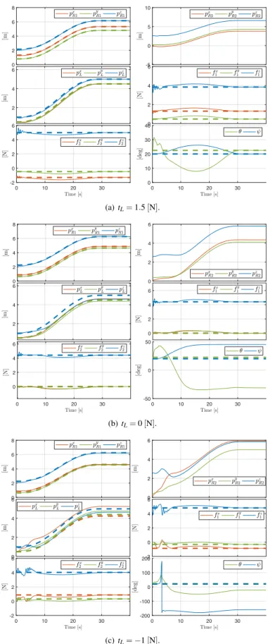
Fig. 1: Evolution of the system variables for tL=1.5 [N] starting from

two different initial conditions. The positions of the robots center of masses (which coincide with the cables attaching points) are shown, together with the position of the load center of mass and its yaw and pitch angles. The reference signals are displayed with dotted lines of the same color.

(12)

Fig. 2: Evolution of the system variables for tL=0 [N] starting from

two different initial conditions.

Fig. 3: Evolution of the system variables for tL= 1 [N] starting from

(13)

V. LOADTRANSPORTATION

Considering a time-varying control input, we defined ⇡A1(t)

such that the master robot follows a 5th-order polynomial trajectory in the three directions (rest to rest with condition of zero acceleration at the initial and final points) starting from an initial position of [1.18 0.72 2.2]>_{[m]. The trajectory}

covers 4[m] along each of the the three directions in 30[s]. The particular ⇡A(t), with ⇡A2(t) = ¯⇡0A2 and ⇡A1(tf) = ¯⇡A10 ,

brings the load in the configuration ¯pL= [4.5 4.5 5.0]>[m],

¯

y = p/9 [rad] and ¯q = p/8 [rad]. In Fig. 5 we show the results of the simulations in ideal conditions. We notice that, once the final input ⇡A1(tf) = ¯⇡0A1 with tL>0[N] is set, the

system successfully transports the load between the two points stopping at the desired configuration, as shown in Fig. 4(a).

For tL=0[N] instead, the final load attitude depends on the

particular motion, and it is in general different from the desired one, as shown in Fig. 4(b). Finally, as one can see in Fig. 4(c),

when tL <0[N] the final configuration of the system does

not correspond to the desired one, since it was an unstable equilibrium. Notice in Fig. 4(a) how the error on the load trajectory remains sufficiently small for all the transportation, and goes to zero at the end of the task. In Fig. 5(a), 5(b)

and 5(c) we show the results for a similar task, for tL>0,

tL =0 and tL <0, respectively. In this case the trajectory

is followed at a higher speed, since it is completed in 4 [s]. Consequently, as one can see in Fig. 5(a), the system moves faster and the tracking error increases. However it remains always bounded and the stability during the transportation is preserved. Furthermore, one could tune the admittance controller parameters of the slave robot to achieve better results if needed. 0 2 4 6 8 -5 0 5 10 2 4 6 0 2 4 6 0 10 20 30 -2 0 2 4 6 0 10 20 30 0 10 20 30 40 (a) tL=1.5 [N]. 0 2 4 6 8 0 2 4 6 2 4 6 0 2 4 6 0 10 20 30 0 2 4 6 0 10 20 30 -50 0 50 (b) tL=0 [N]. 0 2 4 6 8 0 2 4 6 0 2 4 6 -2 0 2 4 6 0 10 20 30 -2 0 2 4 6 0 10 20 30 -200 -100 0 100 200 (c) tL= 1 [N].

Fig. 4: Evolution of the system variables during transportation for the three different values of internal force.

(14)

0 2 4 6 8 -5 0 5 10 0 2 4 6 0 2 4 6 8 0 2 4 6 8 -5 0 5 10 0 2 4 6 8 -20 0 20 40 (a) tL=1.5 [N]. 0 2 4 6 8 0 2 4 6 2 4 6 -5 0 5 10 0 2 4 6 8 -5 0 5 10 0 2 4 6 8 -40 -20 0 20 40 (b) tL=0 [N]. 0 2 4 6 8 0 2 4 6 2 4 6 -5 0 5 10 0 2 4 6 8 -2 0 2 4 6 0 2 4 6 8 -200 -100 0 100 200 (c) tL= 1 [N].

Fig. 5: Evolution of the system variables during transportation for the three different values of internal force.

(15)

Fig. 6: Simulation result with noisy measurements.

VI. NON-IDEALCONDITIONS

In the following, we test the robustness of the proposed method against noise in the measured state and model pa-rameter uncertainties. The following simulations consider the transportation scenario presented in Sec. V, where the trajec-tory is performed in 4[s].

A. Noisy Measurements

In Fig. 6 we report the results of a simulation where Gaussian noise is added to the estimated state of the robots and to the measured cable force, in order to simulate real sensors. In particular, the noise variances on the aerial vehicle position, velocity and measured cable force are equal to 0.005[m], 0.01[m/s] and 0.01[N], respectively. From the plots one can see that, even in the presence of noise, the system is able to bring the load to the desired pose showing only very small oscillations.

B. Noisy Measurements and Parametric Uncertainties In Fig. 7 both measurement noise and parametric uncer-tainties are considered. In particular, the rest length of the cables, the cables anchoring points positions with respect to the center of mass of the load (or equivalently the position of the center of mass of the load) and the mass of the load are uncertain parameters. In other words, we put ourselves in a condition in which the real parameters and the nominal ones do not perfectly match. In particular, the known cables rest length has been set 5% greater than the real one, the

load mass used to generate the constant control input ⇡A

is 20% greater than the real one, and the anchoring points

positions in body frame have been chosen as follows: Lb1=

[0.5 0.01 0.02]>_[m], L_b

2= [ 0.47 0.02 0.03]>[m]. With this

simulation we want to show that the proposed algorithm is robust to uncertainties on the parameters in the sense that the system final equilibrium will be clearly different from the desired one, but the robots are still perfectly capable of performing the object transportation task in a stable way, as guaranteed by the system passivity. Fig. 7 shows the results of the simulation during the transportation. As on can see, the

Fig. 7: Evolution of the main system variables for the transportation can in the presence of noise and model uncertainties.

passive nature of the closed loop system makes the system state and output completely stable and converging to a constant equilibrium, that is of course different from the desired one because of the wrong parameter used. An adaptive approach could be used to reduce the effect of this

C. Sensitivity to Load Mass Uncertainty

We performed several simulations varying the mass of the load known by the controller with respect to the real mass. Figure 8 displays how the load position and attitude errors at steady state, e_Lp and ea

L, change when the real mass is not

exactly known. In particular, the errors are defined as: ep_L=kpL ¯pLk

eaL=||q ¯q||+||y ¯y||.

The load starts from the configuration given by: pL(0) =

[0.5 0.5 1]>_[m], _{y = p/10 [rad] , q = p/8 [rad] and t}_L ₌

1.5 [N]. The desired final configuration is given by ¯pL =

[0.5 0.5 1]>_{[m] , ¯}_{q = p/9 [rad], ¯y = p/8 [rad], t}_L₌_{1.5 [N].}

Calling m0

L the known mass, we compute it as m0L=Dm · mL

where Dm is the relative mass increment. Figure 8 shows

ep_L and ea

L with respect to Dm. The larger the parametric

uncertainty on the load mass, the more the errors increase, too. However one can notice that even with an uncertainty grater than the 25% the system still remains stable. After the

value Dm = 1.3 the system becomes unstable. Nevertheless,

we remark that the mass of the load is one of the parameters that can be known with very good precision, also using an online estimation algorithm.

D. Sensitivity to Anchoring Point Position Uncertainty As an additional study of the robustness of the proposed method, in Fig. 9 we show the load position and attitude errors at steady state when the parametric uncertainty is on Preprint version, final version at http://ieeexplore.ieee.org/ 7 IEEE Robotics and Automation Letters 2018

(16)

0.7 0.8 0.9 1 1.1 1.2 1.3 0 0.1 0.2 0.3 0.4 0.5 0.6 0.7 0.8 0.9 0.7 0.8 0.9 1 1.1 1.2 1.3 0 0.1 0.2 0.3 0.4 0.5 0.6 0.7 0.8 0.9

Fig. 8: Load position and attitude errors when the load mass known by the controller differs from the real one.

the position of the cables anchoring points on the load. In particular, the known anchoring positions are given by

L_b0 1=Lb1+ 2 411 1 3 5DbkL_b 1k L_b0 2=Lb2+ 2 4 11 1 3 5_DbkL_b 1k,

where Db 2 R 0. The system starts from the configuration

given by pL(0) = [0.5 0.5 1]>[m], y = p/10 [rad], q =

p/8 [rad] and tL=1.5 [N]. The desired final configuration is

given by ¯pL= [0.5 0.5 1]>[m] , ¯q = p/9 [rad], ¯y = p/8 [rad],

tL=1.5 [N]. Also in this case, as expected, the larger the

para-metric uncertainty on the considered quantities, the more the errors increase, too. However, with the considerable variation

of Db = 0.5 the system still remains stable.

0 0.1 0.2 0.3 0.4 0.5 0.6 0 0.1 0.2 0.3 0.4 0.5 0.6 0 0.1 0.2 0.3 0.4 0.5 0.6 0 0.05 0.1 0.15 0.2 0.25 0.3 0.35

Fig. 9: Load position and attitude errors when the anchoring points position on the load known by the controller differs from the real one.

(17)

0.1 0.2 0.3 0.4 0.5 0.6 0.7 0.8 0.9 1 2 4 6 8 10 12 14 16 18 20

Fig. 10: Convergence time of the load position and attitude errors

when the tLincreases.

VII. EFFECTS OF THEINTERNALFORCEALONG THE

LOAD

In the manuscript we saw that to make a desired load con-figuration asymptotically stable, one has to compute the proper control input ⇡A(¯q,tL) choosing tL>0. In the following, we

shall analyze the effects of the intensity of the internal force on the system behavior. In this way we can better decide the

value of tL. In particular, in the following, we shall analyze

the relations between tL and convergence time, and between

tL and required total thrust in the equilibrium configuration.

A. Internal Force and Convergence Time

If the internal force tL=0 [N] the load does not in general

converge to its desired pose, which instead happens for tL>0.

However, it is interesting to see how the convergence rate behaves changing the intensity of the internal force. In Fig. 10, we show how the convergence time of the load position and

attitude, defined by tc, varies when increasing the internal

force. Here tc=min{tca,tcp}, where tca is the time after which

ea

L remains below 5 [ ], while tcp is the time after which eLp

remains below 0.02 [m]. The initial and the final desired load

configurations are the same as before. Notice that for tL=0

the convergence time is in general infinite. One can notice

that increasing tL up to 0.7 [N], tc decreases. However, after

this value, tcstarts to increase due to the appearance of some

larger oscillations that takes more time to be damped. In any case, this study shows that even a minimal internal force of 0.1 [N] is enough to obtain asymptotically stability for which an almost negligible increase of total thrust is required. B. Internal Force and Total Thrust

Since the internal force, necessary to make the load verge to the desired pose, implies an additional energy con-sumption for the robots, we evaluated the amount of additional thrust required when the internal force increases. Given a

0 0.5 1 1.5 2 2.5 3 0 0.005 0.01 0.015 0.02 0.025 0.03

Fig. 11: Additional thrust required by the two robots to stabilize the

load when tLincreases.

certain desired load pose, Fig. 11 shows the relative increase

of total thrust, D fR, augmenting the intensity of the internal

force with respect to the total thrust required by the case with

zero internal force. In particular D fRis computed as

D fR(tL) = fR(tL) f 0 R f0 R ,

where fR(tL)is the the sum of the thrusts required by the two

vehicles at steady state to stabilize the load at a certain load configuration with a certain value of tL, and fR0=fR(0).

One can notice that even imposing tL=1 [N], much higher

than the real internal force required to stabilize the system, theD fRis below the 0.005, i.e., the total extra thrust is lower

than the 0.5% of the total thrust required with tL=0 [N].

In any case we remark that the proposed control method

is still applicable for tL=0 [N]. The system is proven to be

still stable, but will not clearly asymptotically converge to the desired pose.

REFERENCES

[1] M. Tognon, C. Gabellieri, L. Pallottino, and A. Franchi, “Aerial co-manipulation with cables: The role of internal force for equilibria, stability, and passivity,” IEEE Robotics and Automation Letters, Special Issue on Aerial Manipulation, 2018.

[2] R. Horst, P. M. Pardalos, and N. V. Thoai, Introduction to global optimization. Springer Science & Business Media, 2000.

[3] K. Eriksson, D. Estep, and C. Johnson, Applied Mathematics Body and Soul: Vol III. Springer-Verlag Publishing, 2003.