A performance comparison of sensitivity analysis methods for building energy models

The final publication is available at: www.springerlink.com

Please cite this article as: Nguyen, A. T., & Reiter, S. (2015). A performance comparison of sensitivity analysis methods for building energy models. Building Simulation, Vol. 8, No. 6, pp. 651-664

1

A performance comparison of sensitivity analysis methods for building

energy models

Anh-Tuan Nguyena_{, Sigrid Reiter}b

a _{Faculty of Architecture, Danang University of Science and Technology, 54 Nguyen Luong Bang,} LienChieu district, Danang, Vietnam

Tel: +84 (0) 511 3841823 Fax: +84 511 3842771

Email: natuan@ud.edu.vn ; arcnguyenanhtuan@yahoo.com

b _{LEMA, Faculty of Applied Sciences, University of Liege, Bât. B52, Chemin des Chevreuils 1 - 4000} Liège (Sart-Tilman) Belgium

Tel: +32 (0) 4 366 94 82 Email: sigrid.reiter@ulg.ac.be

ABSTRACT

The choice of sensitivity analysis methods for a model often relies on the behavior of model outputs. However, many building energy models are “black-box” functions whose behavior of simulated results is usually unknown or uncertain. This situation raises a question of how to correctly choose a sensitivity analysis method and its settings for building simulation. A performance comparison of nine sensitivity analysis methods has been carried out by means of computational experiments and building energy simulation. A comprehensive test procedure using three benchmark functions and two real-world building energy models was proposed. The degree of complexity was gradually increased by carefully-chosen test problems. Performance of these methods was compared through the ranking of variables’ importance, variables’ sensitivity indices, interaction among variables, and computational cost for each method. Test results show the consistency between the Fourier Amplitude Sensitivity Test (FAST) and the Sobol method. Some evidences found from the tests indicate that performance of other methods was unstable, especially with the non-monotonic test problems.

Keywords: Monte Carlo approach; variance-based sensitivity analysis; regression-based

sensitivity analysis; Morris method; comparison

ABREVIATIONS

FAST Fourier Amplitude Sensitivity Test KCC Kendall coefficient of concordance NMBE Normalized mean bias error OAT One-parameter-at-a-time PCC Partial correlation coefficient

2

PEAR Pearson product moment correlation coefficient PRCC Partial Rank Correlation Coefficients

PTAC Packaged terminal air-conditioner RMSE Root mean square error

SA Sensitivity analysis SPEA Spearman coefficient

SRC Standardized regression coefficient SRRC Standardized rank regression coefficient

1. Background and objectives of this study

During the last decades, applications of computer simulation for handling complex engineering systems have emerged as a promising approach. In building science, researchers and designers often use dynamic thermal simulation programs to analyze thermal and energy behaviors of a building so as to achieve specific targets, e.g. reducing energy consumption, decreasing environmental impacts or improving indoor thermal environment (Garber 2009). Consequently, several techniques have been developed so as to support building simulation analysis, including parametric simulation, sensitivity analysis, simulation-based optimization, meta-model analysis, etc. This paper attempts to deal with the issues related to sensitivity analysis (SA).

Sensitivity is a generic concept. SA has been conceived and defined as a measure of the effect of a given input on the output (Saltelli et al. 2004). If a change of an input parameter

X produces a change in the output parameter Y and these changes can be measured, then we

can determine the sensitivity of Y with respect to X (Lam and Hui 1996). This measure of sensitivity can be obtained by calculations via a direct or an indirect approach, or system derivatives such as

 

/



j

X j

S

Y

X

(Saltelli et al. 2004).

The philosophy of SA is that if we understand the relationships and the relative importance of design parameters, we can easily improve the building performance by carefully selecting important design parameters. Several SA methods have been developed during recent years and many of them can be applied to building simulation. Additionally, the relationship between simulation inputs and outputs is often unknown or uncertain due to the complexity of building energy models. This situation raises some questions of how to choose an appropriate SA method for the problem under consideration or whether a SA result is

3

reliable. In this study, several SA methods commonly used in building simulation were employed to assess the significance of various input parameters of some mathematical models and computer building energy models. By comparing the results of SA given by these different methods, this study provides an insight into the reliability (or accuracy) of these SA methods. The global objective of this study is to evaluate and recommend the most reliable SA methods for building energy models, with a particular focus on small residential buildings.

2. A brief overview of SA methods and the state of the art of SA applied to building energy models

There are a number of approaches used in SA which can be distinguished by their methods, purposes, sensitivity indices. Hamby (1994) provided a comprehensive review on SA methods according to which SA methods could be addressed in three groups:

- Those that evaluate the output on one variable at a time (including 6 methods);

- Those that are based on the generation of a sample of input vectors and associated outputs (including 10 methods);

- Those that perform a partitioning of a particular input vector based on the resulting output vector (including 4 methods).

According to Frey et al. (2003), SA methods may be broadly categorized into three groups as follows:

- The “mathematical approach” typically involves calculating the output for a few values of an input within its possible range. This approach basically consists of the Nominal Range Sensitivity Analysis Method, the Differential Sensitivity Analysis, the method of Morris, most of the methods using the one-parameter-at-a-time (OAT) approach…

- The “statistical (or probabilistic) approach” involves running of a large number of model evaluations on an input sample which is usually generated randomly. Depending upon the method, one or more inputs are varied at a time. The statistical methods allow quantifying the effect of simultaneous interactions among multiple inputs (Frey et al. 2003). The statistical approach includes: the linear Regression Analysis (RA), the analysis of variance (ANOVA), the Response Surface Method (RSM), the Fourier Amplitude Sensitivity Test (FAST), the Mutual Information Index (MII), Sobol’s method, methods using statistical indices: PEAR (Pearson product moment correlation coefficient), SPEA (Spearman coefficient), SRC (Standardized regression coefficient), and SRRC (Standardized rank regression coefficient)… - SA methods using “graphical assessment” to estimate a qualitative measure of sensitivity using graphs, charts, or surfaces of pairs of inputs – corresponding outputs. It can

4

be used to strengthen the results of other quantitative methods for better interpretation. The most common forms of “graphical assessment” are the Scatter Plot and the Regression Analysis.

Heiselberg et al. (2009) grouped SA methods into three classes: ‘local’ sensitivity

methods, global sensitivity methods, and screening methods. ‘Local’ sensitivity methods are

also often based on the OAT approach in which the variation of model outputs is considered under the variation of one design parameter, while all other parameters are held constant. In the global sensitivity approach, the significance of an input factor is evaluated by varying all other input factors as well. These SA methods usually generate a large number of input vectors and model evaluations. Screening methods are used to reduce computational cost in high-dimensional or computationally expensive models. In these methods, the significance of each input is evaluated in turn and the sensitivity index is evaluated by the average of the partial derivatives at different points in the input space. The method of Morris (1991) is one of the most commonly used screening methods.

In building research, SA is often quantified by the difference in simulated results caused by the variations of input parameters. A SA provides designers a robust tool to quantify the effect of various design parameters and to identify sources of uncertainty. Lomas and Eppel (1992) examined performance of 3 SA methods (Differential sensitivity analysis, Monte Carlo analysis, and Stochastic sensitivity analysis) on 3 building energy programs (ESP, HTB2, and SERI-RES). The variation of simulation outputs were caused by the perturbation of 70 input parameters. The study indicates that both Differential sensitivity analysis and Monte Carlo analysis yielded similar results and could be applied to the widest range of thermal programs while Stochastic sensitivity analysis was complex to implement. Lam and Hui (1996) performed a study on the effects of various design parameters on building energy consumption. They used a simple ‘local’ sensitivity test and the simulation tool DOE-2 to examine an office model in Hong Kong. As the variation of each design parameter was considered separately, their study could not quantify complex interactions among design parameters. The results were therefore unconvincing. Heiselberg et al. (2009, p. 2036) used the Morris method (Morris 1991) - a local sensitivity method - to perform SA for an office building in Denmark to measure the influence of design parameters on total building energy demand. They concluded that “SA in the early stages of the design process can give important

information about which design parameters to focus on in the next phases of the design” and

5

performance”. Hopfe and Hensen (2011) performed uncertainty analysis and SA on three

groups of input parameters of an office building, including: physical parameters, design parameters and scenario parameters. The perturbation of input parameters was generated by the Latin hypercube sampling (LHS) method and the Standardized Rank Regression Coefficient (SRRC) was used as the quantitative measure of sensitivity. This study revealed that the infiltration rate and the room geometry were among the most sensitive parameters of the model. By investigating the models of two office buildings, Eisenhower et al. (2011, p. 2785) found that “the most sensitive parameters of the model relate to building operation (i.e.

scheduling), and also find that a low energy building design is more robust to parameter variations than the conventional design”. In Eisenhower et al. (2012), the authors proposed

and applied a decomposition of sensitivity indices to quantify which intermediate processes (e.g. Air handling unit, heating sources, cooling sources…) contributed the most to the uncertainty of building simulation outputs.

The above mentioned studies show a preliminary insight of the importance and applications of SA among building research communities. This study investigates capability of three common global SA methods and a screening method with a total of nine sensitivity measures, as described in Table 1. The categorization in Table 1 is similar to the work of Tian (2013) and will be used hereafter.

Table 1: SA methods investigated in this study and their basic features (adapted from (Morris 1991; Sobol 1993; Hamby 1994; Frey et al. 2003; Giglioli and Saltelli 2008; Tian 2013; Saltelli et al. 2004; Nossent el al. 2011))

Regression-based sensitivity indices (Nguyen 2013; Yang 2011; Calleja Rodríguez et al. 2013)

1. PEAR PEAR measures the usual linear correlation coefficient between Y and a given input Xj. This sensitivity index is strictly applied to linear models. 2. SRC SRC gives the strength of the correlation between Y and a given input Xj

through a linear regression model having the form

i j ij i

j

y  a



Reliability of the SRC strongly depends on the R2 _{of the linear model.} 3. PCC PCC gives the strength of the correlation between Y and a given input Xj

cleaned of any effect due to any correlation between Xj and any of the Xi

6

based either on SRC’s or PCC’s (in their absolute values) is exactly the same. Regression-based sensitivity indices (using rank transformation techniques) (Nguyen 2013; Hopfe and Hensen 2011)

4. SPEA SPEA is essentially the same as PEAR, but using the ranks of both Y and Xj instead of the raw values, i.e.: SPEA(Y,Xj) = PEAR[R(Y),R(Xj)]

where R(*) indicates the transformation which substitutes the variable value with its rank.

5. SRRC SRRC is used instead of SRC when R2 _{is low. In this case, the input and} output variables are replaced by their ranks, and the regression is then performed entirely on these ranks. SRRC is better than SRC if the model output varies non-linearly, but monotonically with each independent variable.

6. PRCC PRCC is the PCC calculated on the rank of input variables. The

performance of the PRCC shows the same features of performance as the SRCC: good for monotonic models, and not fully satisfactory in the presence of non-monotonicity. Variance-based sensitivity methods (Mara and Tarantola 2008) 7. Sobol index

Both Sobol and FAST methods are model-independent approach in SA. They decompose the variance of model outputs into fractions which can be attributed to inputs or sets of inputs. These methods can deal with

nonlinear and non-monotonic models or models with strongly correlated inputs. For each method, two measures of SA can be used:

- "First-order sensitivity index": is the contribution to the output variance of the main effect of Xi, hence it measures the effect of varying Xi alone, but averaged over variations in other input parameters.

- "Total-effect index": measures the contribution to the output variance of Xi, including all variance caused by its interactions, of any order, with any other input variables.

8. FAST* sensitivity index Screening-based method (Heiselberg et al. 2009) 9. Morris’s SA method

Morris method is also a model-independent approach in SA. It computes partial derivatives of a model at evenly-distributed points (often called “level”) within input ranges and these derivatives are then average out. Morris method gives 2 indicators related to SA: one (μ) is to estimate the main effect of the input factor on the output and the other (σ) is to assess the interaction with other factors or the nonlinear effects. This method does not support uncertainty analysis.

* This study uses the extended FAST method which allows calculations of both first and total-order sensitivity indices.

The selection of SA methods for a model requires some knowledge of the model output. In practice, it is not easy to know output behavior of a model, especially building energy models. Many studies have indicated that building simulation outputs are generally nonlinear, multimodal, discontinuous (Nguyen et al. 2014; Kampf et al. 2010), thus non-differentiable

7

and non-monotonic. These features generally cause many challenges for some SA methods. Moreover, variance-based SA methods, e.g. the Sobol method, need a large number of model evaluations to calculate sensitivity indices, whereas building energy models are generally computationally expensive. Therefore, there exists a growing concern about the relevancy of a SA method for a building energy model and how reliable a method is. The next sections of this paper present a test procedure and the SA results which provide some insight into this concern.

3. Methodology

This work performs global SA using the sampling-based approach. This approach is also referred to as the “Monte Carlo-based method”. A Monte Carlo-based SA provides statistical answers to a problem by running multiple model evaluations with a probabilistically generated input sample, and then the result of these evaluations are used to determine the sensitivity indices (Giglioli and Saltelli 2008). In this paper, the Monte Carlo-based SA consists of five major steps as follows (Mara and Tarantola 2008):

- Select the model to perform SA;

- Identify simulation inputs of the model that should be included in the SA and the probability distribution functions of these variables;

- Generate a sample of N input vectors for the model using a probability sampling method;

- Run the simulation model N times on the input sample to produce N corresponding outputs;

- Calculate the sensitivity indices for each input and draw necessary conclusions.

3.1 Sampling methods

In step 3, the input samples are generated by some sampling strategies. The calculation of the Sobol sensitivity indices imperatively needs the input sample generated by the Sobol sequence (Sobol 2001). For the FAST method, the FAST sampling method (Cukier et al. 1978) is required. The modified Morris method generates its input sample by the Morris sampling strategy (Morris 1991). For the regression-based SA, some sampling methods can be applied. We observe that several SA studies employed the LHS method to generate input samples (Kotek et al. 2007; Hopfe Hensen 2011, Cosenza et al. 2013). They stated that the enforced stratification over the range of each sampled variable gives the LHS a desirable property for SA and uncertainty analysis. Particularly, Helton et al. (2005) compared the SA

8

results obtained by different sampling strategies and they recommended the LHS. Thus, the LHS was used in our study.

The number of model evaluations (sample size) needed for a reliable Monte Carlo analysis must be large enough to assure convergence of the sensitivity indices, but should not be too large to delay the SA process. There are some basic principles for choosing the sample size of each SA method. For the FAST and Sobol methods, the sample size depends on the number of variables and the sampling method used (see (Saltelli and Bolado 1998) for further description of the sample size). The smallest sample size for the Sobol indices (both first and total-order indices) is n(2k+2), where n is the minimum model evaluations for estimating one individual effect; n takes the value of 16, or 32, 64…; k is the number of variables. The smallest sample size for the FAST indices is 65k; k is the number of variables (Giglioli and Saltelli 2008). The number of model evaluations for Morris μ* is r(k+1), where r is the number of trajectories (depends on number of levels, r is usually taken between 5 and 15 – see (Morris 1991)). We examined the result of the Morris method with different levels and sample sizes. For the regression-based sensitivity indices, although no explanation was mentioned, SimLab (Giglioli and Saltelli 2008) recommends the sample size of 1.5 up to 10 times the number of input variables. In Monte Carlo analysis, Lomas and Eppel (1992) found that only marginal improvements in accuracy are obtained after 60-80 simulations; we therefore started the convergence test using the small sample size (40 simulations). As time for a model evaluation is negligible, we generated a large number of sample sets of input variables and see the variation of sensitivity indices calculated by the SA methods under consideration. Totally, 269117 function evaluations were done for the test. By examining the evolution of sensitivity indices as a function of the sample sizes, the convergence behavior and capability of the SA methods were derived.

3.2 Test models and tools

The test models are three benchmark functions and two real-world building energy models in EnergyPlus.

3.2.1 Description of the test functions

The performance of nine sensitivity measures (in Table 1) was tested using three benchmark functions. They were chosen from the literature in such a way that they provide increasing challenges to the SA methods by their increasing level of complexity. The objective of the test with these functions is (i) to examine the convergence behavior of the nine sensitivity indices calculated by the SA methods; and (ii) partly to compare the

9

performance of the nine SA methods. Six independent variables were examined. This number was kept unchanged in all tests because six variables will be relevant to the tests with computationally-expensive building models. All variables were considered continuous and their probability distribution functions are uniform (Saltelli and Bolado 1998; Archer et al. 1997; Campolongo et al. 2000; Helton and Davis 2002).

The first test function is a linear function (Model 3, reference (Campolongo et al. 2000; Helton and Davis 2002)) which is defined by:

1

1

( )

(

)

2

f x

c x







with

x



U

(0,1)

of xi is proportional to the value of ci, which is inversely proportional to i. Thus, the correct

order of variables’ importance should be x1, x2, x3, x4, x5, x6.

The second test was performed using a monotonic function (Model 5, reference (Campolongo et al. 2000; Helton and Davis 2002)) which is defined by:

1 1

( )

exp(

)

(

1) /

f x

b x

e

b











with

x



U

(0,1)

= 0.1. For this function, the importance of variables xi is proportional to its coefficient bi. By

setting bi to the values above, the correct order of variables’ importance should be x1, x2, x3,

x4, x5, x6.

The third test was performed using a strongly nonlinear non-monotonic function, namely the “g-function” (Model 7 in reference (Campolongo et al. 2000), (Saltelli and Sobol 1995; Saltelli and Bolado 1998; Archer et al. 1997; Helton and Davis 2002)), which is defined by:

1 1 4 2 ( ) ( ) 1 n n i i i i i i _i x a f x g x a       





The function f(x) is defined in an n-dimensional unit cube -

x



U

(0,1)

4.5, a4 = 9, a5 = a6 =99.

It is easy to prove that the function gi(xi) varies as

1

1

1

( ) 1

1

a

g x

1

a





 

10

For this reason, the size of ai determines the sensitivity of the function to the variation of

variable xi. For example:

- If ai = 0 then

0



g x

( )



2

- If ai = 9 then

0.9



g x

( ) 1.1



xi;

- If ai = 99 then

0.99



g x

( ) 1.01



This relationship is illustrated in Figure 1.

Figure 1: Plot of the function gi(xi), for different values of the coefficient ai

The g-function is a challenge to the SA methods since it allows an automatic tuning of the relative importance of variables, as well as their interactions (by definition, all interaction terms are non-zero) by using appropriate values of ai.

There are some advantages to the use of these test functions, including: - Clear specification of the model under consideration;

- Three different functions allowed the authors to vary the level of difficulty of the tests;

- Function evaluations and sensitivity indices could be computed analytically;

- Low computational cost that allows testing the influence of different sample sizes on the SA results (the convergence of the sensitivity indices);

- These functions have both linear and nonlinear, monotonic and non-monotonic response, thus they provide good test arena for the SA methods;

These three tests allowed the authors to compare the results with each other.

3.2.2 Test A: thermal model of a naturally-ventilated apartment

The selected building is located near the centre of Danang, Vietnam where the climate is warm and humid all year round. This seven-storey condominium, which was built in 2010, is

11

a typical dwelling designed for low income residents. The apartment has a gross floor area of 53 m2 with two small bedrooms and is located on the 4th floor at a corner of the building (see Figure 2). The EnergyPlus model of this apartment was established and carefully calibrated by in-situ monitoring data. The simulated and monitored indoor temperature was in good agreement. The normalized mean bias error (NMBE) and the root-mean-square error (RMSE) of the model were 0% and 1.41%, respectively (see (Nguyen and Reiter, 2012; Nguyen 2013)). As the whole building is naturally ventilated, indoor thermal comfort of occupants is obviously the greatest concern. The comfort assessment method in this EnergyPlus model was based on the adaptive thermal comfort theory and the result of a comprehensive meta-analysis conducted by the authors (Nguyen et al. 2012). The implementation of this comfort model into EnergyPlus was carefully described in (Nguyen and Reiter 2014; Nguyen 2013). In this test, we examined the sensitivity of the discomfort period (total time - in hour - when the comfort criterion is not met) caused by the variation of 6 passive design parameters as listed in Table 2 (in random order). The ranges of these parameters were defined according to common passive design solutions of designers. For example, size of the window overhang could be 0 (no overhang) to 0.8 (large overhang in a common design); and the possibility of 0 or 0.8, or any other value in the range [0, 0.8] is equal. For these reasons, the probability distribution function of all 6 parameters was set as uniform. These settings were used in some previous studies (Nguyen 2013; Nguyen and Reiter 2014). Among these six parameters, we intentionally chose 3 discrete parameters so as to challenge the SA methods. The number of parameters was limited to 6 due to computationally expensive simulations and large sample sizes, especially in the tests of the variance-based methods.

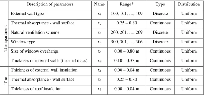
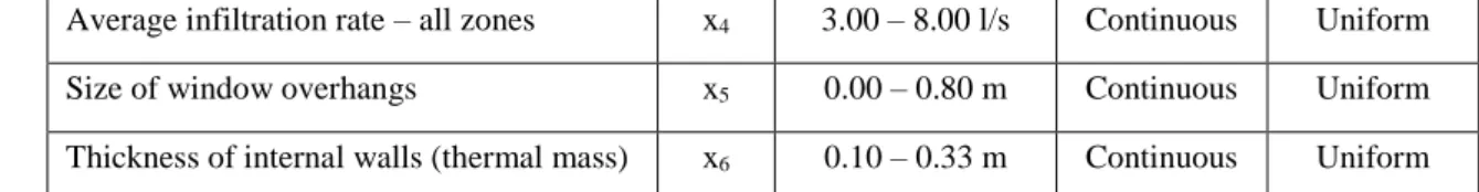
Table 2: Parameters and parameter ranges used in sensitivity analysis

Description of parameters Name Range* Type Distribution

T h e ap ar tm en t

External wall type x1 100, 101, …, 109 Discrete Uniform

Thermal absorptance - wall surface x2 0.25 – 0.80 Continuous Uniform

Natural ventilation scheme x3 200, 201, …, 209 Discrete Uniform

Window type x4 300, 301, …, 306 Discrete Uniform

Size of window overhangs x5 0.00 – 0.80 m Continuous Uniform

Thickness of internal walls (thermal mass) x6 0.10 – 0.33 m Continuous Uniform

T h e d etac h ed h o u se

Thickness of external wall insulation x1 0.00 – 0.04 m Continuous Uniform Thermal absorptance - wall surface x2 0.25 – 0.80 Continuous Uniform

12

Average infiltration rate – all zones x4 3.00 – 8.00 l/s Continuous Uniform

Size of window overhangs x5 0.00 – 0.80 m Continuous Uniform

Thickness of internal walls (thermal mass) x6 0.10 – 0.33 m Continuous Uniform * For discrete parameters, each number represents a codified name of building components or ventilation schemes in EnergyPlus (e.g. 101 means “220mm brick wall - no insulation or air gap”)

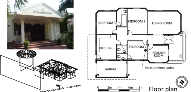
Figure 2: Details of the selected building and the apartment (test A) 3.2.3 Test B: energy model of an air-conditioned detached house

The detached house situated near the seashore of Danang is being occupied by a family of 4. This house is surrounded by a garden; thus it is completely isolated from other buildings (see Figure 3). The house has 4 free-running zones (2 toilets, the roof attic and the corridor) and 6 climate-controlled zones by using 6 packaged terminal air-conditioners (PTAC). Each PTAC consists of an electric heating coil, a single-speed cooling coil, a ‘draw through’ fan, an outdoor air mixer, a thermostat control and a temperature sensor. It was assumed that the heating coil efficiency is 1; the coefficient of performance (COP) of the cooling coil is 3; the efficiency of the fan blades and the fan motor are 0.7 and 0.8 respectively; heating and cooling supplied air temperatures of the PTACs are 50°C and 13°C. Other features (e.g. flow rates, power of the coils) of these components are automatically estimated by EnergyPlus to meet thermal loads of the zones when design parameters vary. Energy consumption of a PTAC is the sum of heating, cooling, and fan electricity. The simulated result for SA tests was the annual energy consumption of the house which is the sum of electricity consumed by the lighting system, equipments and the PTACs. The thermal model of this house was carefully calibrated to achieve the NMBE of -0.16% and the RMSE of 1.13% (see (Nguyen 2013)).

BEDROOM 2 BEDROOM 1 BALCONY TOILET LIVING ROOM Apartment plan 0 1 5m Position in building Measurement point

13

Figure 3: Details of the selected detached house and its 3D EnergyPlus model (test B)

In this SA test, we intentionally selected 6 passive design parameters (see Table 2 - in random order) which were nearly consistent with those of the apartment, but their values vary continuously. The aim is to generate a new test challenge as well as to facilitate comparison of the results between the two cases and to building design rules of thumb under the warm humid climate.

3.2.4 Sensitivity analysis tool

Both SimLab 2.2 (Giglioli and Saltelli 2011) and Dakota (Adams et al. 2009) can be used (free of charge) to perform SA. This study chose SimLab due to its simplicity and its user-friendly interface. Input sampling and output processing are done with the support of SimLab. SimLab directly interacts with the three benchmark functions through Microsoft Excel®. SimLab interacts with EnergyPlus through a special interface developed by the authors, allowing to automatically extract the results from thousands of EnergyPlus output files and to convert them into a predefined format readable by SimLab. This SA process is summarized and illustrated in Figure 4.

0 .6x 0 .8 LIVING ROOM READING BEDROOM 1 BEDROOM 2 BEDROOM 3 KITCHEN GARAGE

Floor plan

14

Figure 4: The full process of a SA using SimLab and EnergyPlus

3.3 Assessment criteria and Sensitivity indicators of the SA methods

The modified Morris method (Campolongo el al. 2007) gives two sensitivity indicators, including the main effect μ* and the nonlinear effect σ (interaction with other variables). We consider μ* as the Morris indicator of sensitivity (see (Confalonieri et al. 2010)) and σ as the indicator of interaction.

Each SA method will calculate and assign a sensitivity index to each input variable and its corresponding ranking. As sensitivity indices of different SA methods may not use the same metric, we decided to evaluate the performance of these SA methods using following comparisons and methods:

- Compare variables’ sensitivity rankings to that of the reference method (qualitative comparison) using Kendall’s coefficient of concordance;

- Compare variables’ degree of importance to that of the reference method (quantitative comparison) using the ‘normalized sensitivity value’;

- Compare methods’ capability to detect interaction among input variables by considering both the sensitivity term and interaction term of the SA result;

- Compare methods’ capability to provide results in reasonable amount of time by monitoring their convergence behavior.

15

4. Results

4.1 Results of the SA tests with three benchmark functions

Results of the test with the three test functions are presented in Figure 5, Figure 6, and Figure 7. For the linear function and the monotonic function, Figure 5 shows that the PEAR, PCC (Partial correlation coefficient) and SRC needed about 140 function evaluations to achieve stable solutions. Their solutions after 140 runs and those after 800 runs were likely the same. This number of simulations - 140 - was slightly higher than that proposed by Lomas and Eppel (1992). This is possibly because the “total sensitivity index” of Lomas and Eppel relies on the standard deviation of output samples, whereas the PEAR, PCC and SRC are derived by input-output linear regressions. The similar convergence behavior of the PEAR, PCC and SRC is understandable because all these indices are intrinsically calculated using the Pearson product moment correlation coefficient. Among them, the SRC was the most stable. Contrary to the stability of the PEAR, PCC and SRC, all the rank transformation SA indices - SPEA, PRCC (Partial Rank Correlation Coefficients) and SRRC - showed significantly changes of their values between the run 400th and 600th. Their solutions can be considered stable after the run 800th. It is worthy of note that the solutions of the rank transformation SA indices before convergence are completely incorrect, thus the convergence is crucial for their accuracy.

For the g-function, all the regression-based sensitivity indices showed fluctuated outcomes and finally they failed to produce correct predictions of variables’ sensitivity, even at the large sample sizes. The performance of the regression-based sensitivity indices is normally satisfactory if the model output varies linearly or at least monotonically with each independent variable. Nevertheless, if the model is strongly non-monotonic, the accuracy of results may become dubious or completely misleading (Giglioli and Saltelli 2011). The strong non-monotonicity of the g-function is believed to be the reason of this failure.

17

Figure 5: Evolution of the regression-based sensitivity indices as a function of the sample sizes

18

Figure 6: Morris μ* as a function of sample sizes and levels (the red circles show the incorrect prediction of the Morris method for variable x3)

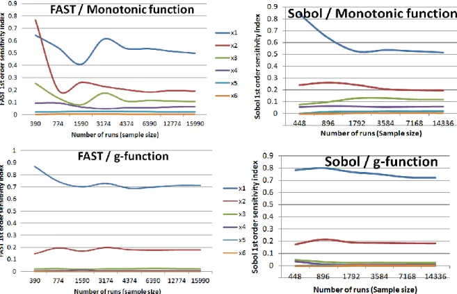
19

Figure 7: FAST and Sobol first order sensitivity indices as a function of sample sizes Figure 6 presents the performance of the modified Morris method with 6 different input samples for the three test functions. In most cases, the method gave fairly stable predictions which resulted in correct rankings of variables’ importance. Different from the regression-based methods, the method of Morris was able to deal with the strong non-monotonicity of the g-function. This is because the Morris µ* of each input is estimated by averaging local derivatives (elementary effects) of the function which are separately calculated at different points within the input range, thereby overcoming the non-monotonicity of the function. However, it still failed two times in predicting the importance of x3 (see Figure 6). By

investigating the input samples of these two cases, we found that these failures were possibly caused by the random sampling which resulted in uneven distribution of input vectors on the designed levels within the range of x3. Among the samples that gave reasonable predictions

(4 levels – 49 inputs; 8 levels – 49 inputs; 4 levels – 70 inputs; and 6 levels – 70 inputs), we considered “6 levels and 70 input vectors” as the optimum setting for the next tests because this setting offers a balance between the number of levels and inputs (theoretically, a high number of levels to be explored needs to be balanced by a high number of trajectories (thus a large sample) in order to obtain an exploratory sample – see the number of model evaluations in section 3.1).

20

The outcomes of the FAST and Sobol method are shown in Figure 7. It is observed that in some tests, the predictions of these two methods suffer from small sample sizes (e.g. smaller than 1000). For the three test functions, FAST sensitivity indices can be considered stable if the sample size is equal or larger than 4374. Sobol sensitivity indices converged to stable solutions if the sample size is equal or larger than 3584. Both the FAST and Sobol methods had no problem with the g-function. In all tests, they gave reasonable predictions after convergence. Because of the space constraint, the total sensitivity indices of Sobol and FAST are not shown, but in our tests their convergence behavior was similar to that of the first order indices.

Through the series of tests, we found that the sample sizes vary from one SA method to another, but is seems that the sample size needed for each method is fairly independent from the test problem. For six independent variables, the PEAR, PCC, and SRC need only 140 function evaluations; the SPEA, PRCC, and SRRC need at least 800 function evaluations; the Morris method only requires 70 evaluations; the FAST and Sobol method require 4374 and 3584 evaluations, respectively.

The performance of the SA methods was not uniform, in terms of stability, accuracy and number of simulations required. The FAST and Sobol method outperformed the others in these tests, except their high number of simulations. They provided correct rankings as well as reasonable variables' importance with respect to variables’ coefficients. According to the literature (Saltelli et al. 2004; Campolongo et al. 2007; Saltelli et al. 1999) the variance-based measures can be regarded as good practice in SA and they can be considered as truly quantitative methods for numerical experiments. Based on many studies found from the literature that used or supported the Sobol method as the reference method (Saltelli and Bolado 1998; Ridolfi 2013; Massmann and Holzmann 2012; Wainwright et al. 2013; Confalonieri et al. 2010; Campolongo et al. 2007; Yang 2011), the Sobol method was considered the reference method for further investigations.

4.2 Results of the SA test with real-world building energy models

In SA with building energy models, the convergence of different sensitivity indices has not been fully understood. The results in section 4.1 reveal that the sample size needed for each SA method is fairly independent from the test function. The sample size for each SA method was therefore determined as follows: 3584 for the Sobol method; 4374 for the FAST; 140 for the PEAR, PCC, and SRC; 800 for the rank transformation SPEA, PRCC, and SRRC; and 70 inputs on 6 levels for the Morris method. Thus, for each model, the SA required 8968

21

simulations. As each simulation completed in around 1 to 2 minutes on our computer (CPU Intel core i5 4x2.53GHz and 4Gb RAM), the total simulation time was about 10 consecutive days (two simulations could run on the system concurrently).

As explained in section 4.1, we compared results of the Sobol method (as the reference method) with that of the remaining methods. In out tests, as the Sobol method and the FAST provide both first and total order sensitivity indices and the differences between the two indices were small, we only present the first order sensitivity index in the comparison.

4.2.1 Qualitative comparison using sensitivity rankings

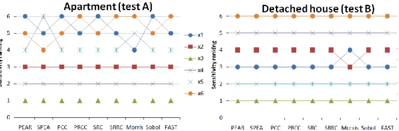
First, we compared the sensitivity rankings of the design parameters given by these SA methods. Figure 8 shows the rankings of different SA methods which were not consistent in the test A, but almost consistent in the test B. In the test A, the inconsistencies mainly occurred to the lowest ranked parameters (ranked 4th, 5th, and 6th), e.g. x1, x5, and x6. All the methods

are consistent in predicting positions of the highly ranked parameters (ranked 1st, 2nd, and 3rd), namely x3, x4, x2. The discrete parameters often cause the simulation output non-monotonic

and produce noise to the problem; thus they are possibly the reason of the disagreement among the SA methods. A similar phenomenon was observed in another SA study in which the problem of SA with discrete inputs disappeared if the value of discrete variables were appropriately rearranged (Nguyen 2013, p. 231). In the test B, all parameters are continuous, thus the SA results were more stable. All the methods were in good agreement except that the Morris method failed to predict the rankings of x1 andx2.

Figure 8: Sensitivity rankings of the design parameters by nine sensitivity indices

The Kendall’s coefficient of concordance (KCC) and its test of statistical significance (Kendall and Smith 1939; Helton et al. 2005) were used to assess the agreement between the ranking of a SA method and that of the Sobol method. The KCC is suitable for comparison

22

with a small number of parameters. The KCC ranges from 0 (no agreement) to 1 (complete agreement). In our case, the KCC can be described as follows:

Suppose that parameter xi is given the rank ri,j by the SA method j where there are in total

n parameters and m SA methods to compare. Then the total rank of parameter xi is:

, 1 m i i j j

R

r





And the mean value of these total ranks is:

1

(

1)

2

R



m n



And the KCC is defined as:

2 2 3 1

12

(

)

/

(

)

KCC

R

R

m n

n



_{ }

_



_



_{ }



_







The ranking agreement between a SA method and the Sobol method is reported in Table 3. Table 3 indicates that the PEAR, PCC, and SRC were better than the SPEA, PRCC, SRRC, and FAST in the test A, but they were equally accurate in the test B. The KCCs of the PEAR, PCC and SRC consistently achieved 1 in the two tests, indicating that their ranking results were completely identical with that of the Sobol method. In terms of sensitivity rankings, the Morris method showed the lowest reliability due to its lowest KCCs. We performed chi-square tests to see whether an observed value of KCC is significant, using the test method of Kendall and Smith (1939). All significance tests return p-value lower than 0.05 (all KCCs were statistically significant).

Table 3: The KCC of the SA methods

PEAR SPEA PCC PRCC SRC SRRC Morris FAST

Apart- ment KCC 1 0.91428 1 0.97143 1 0.97143 0.91428 0.97143 p-value 0.0143 0.01917 0.0143 0.01576 0.0143 0.01576 0.01917 0.01576 Detached house KCC 1 1 1 1 1 1 0.97143 1 p-value 0.0143 0.0143 0.0143 0.0143 0.0143 0.0143 0.01576 0.0143

4.2.2 Quantitative comparison using “Normalized sensitivity value”

It is worthy of note that qualitative comparison using variables’ rankings can reveal only part of the intrinsic difference among the results. Hence, we performed another comparison

23

in a more quantitative way. We proposed to use the “normalized sensitivity value” S’ which is defined as:





,

,...,

S

S

max S

S

S



where Si is the sensitivity value of parameter xi; for i = 1, 2, …, n.

The use of the normalized sensitivity value S’ allows us to adjust sensitivity values measured on different scales to a notionally common scale, namely the scale [0,1]. The “normalized sensitivity value” of a parameter ranges from 0 (unimportant) to 1 (the most important parameter). On this scale, we could directly compare the sensitivity indices of the SA methods with those of the Sobol method.

Figure 9: Quantitative comparison of normalized sensitivity values of 6 parameters given by the SA methods

Figure 9 plots the normalized sensitivity values of all the SA methods under consideration. In terms of accuracy, comparison in Figure 9 reveals the followings:

- The FAST and Sobol method yielded similar SA solutions – as observed and reported by Saltelli and Bolado (1998);

- There was a big difference between the results of the variance-based methods and the remaining methods. Compared with the FAST and Sobol method, other methods overestimated the relative importance of many parameters; the results of these methods were inconsistent. The PCC and PRCC gave the worst predictions in the test B;

- Despite using only 70 simulations, performance of the Morris method was seen as equivalent to the regression-based SA methods, with respect to the results of the FAST and Sobol method;

Through the comparison in Figure 9, it can be said that one SA method may show good performance in sensitivity rankings, but its sensitivity indices may expose inaccuracy,

24

compared to a reference method. The regression-based methods were used several times in the literature. As an example, some studies (Yang 2011; Rodríguez et al. 2013) employed the SRC for SA, but these studies did not provide any specific justification for the choice of the SRC. In our tests, all the rank transformation-based sensitivity indices (SPEA, PRCC, and SRRC) did not give any outstanding result, but the PRCC and SRRC can be easily found from the literature on SA applied to building energy models, e.g. in (Hopfe and Hensen 2011; Kotek et al. 2007; Nguyen 2013; Hopfe et al. 2007).

4.2.3 Other comparisons

In terms of capability of quantifying interaction among the input parameters, we examined the results of the Morris method, the Sobol method and the FAST in Figure 10. For the Sobol method and the FAST, the interaction of each input parameter was estimated by the difference between its first-order and total-order sensitivity index. The Morris method is able to detect interaction among input parameters through the Morris σ. Other methods do not quantify or detect interaction among parameters. In the test A, all these three methods showed fairly good agreement. In the test B, the Sobol method showed deviation from the Morris method and the FAST in predicting the interaction term of x3. Through this comparison, we

observed that the Morris method could detect interaction among input parameters with only a small number of simulations.

25

In terms of computational cost, as time for data processing is assumed identical among the SA methods we only compared the time needed for simulation as shown in Figure 11. We estimated computational cost based on the number of simulations needed to achieve stable solutions. Both the Sobol method and FAST required much more time than the remaining methods. In our test cases, the Sobol method and FAST both required from 30 to 72 hours only for the simulation task while the Morris method needed only 1 hour. The simulation time for the PEAR, SRC, and PCC was about 2 hours. If our tests used more than 6 variables, we believe that the computational cost for the SA methods would accordingly increase. It is obvious that the Sobol method and FAST are not really relevant in the practice of building simulation due to their extremely expensive computational cost, unless these methods are supported by sophisticated techniques (e.g. machine learning methods).

Figure 11: Estimated computational cost of different SA methods

5. Summary and conclusions

A comparison of the performance of nine sensitivity indices, including the Sobol method, the FAST, the Morris method, PEAR, SPEA, PCC, PRCC, SRC, and SRRC has been carried out by means of computational experiments and building energy simulation. These indices were applied to different test cases at different levels of difficulty. We applied a comprehensive test procedure which allows us to quantify many features of these SA methods.

The FAST and Sobol method produced similar SA results and their results were consistent in all tests. Nevertheless, they are computationally expensive methods.

In our study, the PEAR, PCC, and SRC could give more reliable results than those of the SPEA, PRCC, and SRRC. The PEAR, PCC, and SRC provided good sensitivity ranking, but they did not provide fully accurate sensitivity indices, compared with the variance-based methods. On the other hand, there were clear evidences to believe that the regression-based

26

sensitivity indices encountered difficulty with monotonic problems while non-monotonicity may present in a building energy model.

In SA of building energy models, expensive computational cost may be the most important obstacle that impedes the application of the variance-based SA methods. The Morris method and regression-based methods appear thus to be the possible choices for SA. From the limited experience of the present study, the PEAR, PCC and SRC can be applied to SA of building energy models. These choices are a compromise between accuracy and computational cost. This study does not recommend the sensitivity indices relying on rank transformation techniques, e.g. the PRCC, SRRC, and SPEA, as they did not exhibit any outstanding feature. Another issue of the rank transformation sensitivity indices is that they alter the model under investigation during their calculation, thereby resulting in sensitivity information of a different model. The new model is not only more linear but also more additive than the original one. They are likely qualitative measures of sensitivity (Giglioli and Saltelli 2008). As the computationally cheapest method of all, the Morris method showed acceptable capability in quantifying sensitivity and interaction among parameters, but it was not reliable in ranking variables’ importance; thus it can be used to classify and to screen out unimportant variables of a model to reduce the complexity of the problem. This evaluation was also confirmed in some other studies (Confalonieri et al. 2010; Wainwright et al. 2013).

One important finding of this study is that the sample size for different SA methods is not trivial as the SA result is sensitive to this value, as shown in section 4.1. It should be defined by testing the independence of SA solutions from the sample size.

Through this paper, we expected that researchers would have a reliable basis to choose an appropriate SA method for their problem. The choice should be based on the features of the problem, the number of independent parameters, length of time for function evaluation and required precision of the result. Furthermore, performance of many SA methods is sensitive to test problems, as shown in this study. Knowledge and understanding about the SA methods is therefore important in order to draw correct conclusions. Our tests were performed with only 6 independent variables, thus we still have a question whether these numbers have any influence on the sample size required and the SA results.

27

Adams BM, et al. (2009). DAKOTA, A Multilevel Parallel Object-Oriented Framework for Design Optimization, Parameter Estimation, Uncertainty Quantification, and Sensitivity Analysis: Version 5.0 User's Manual. Livermore CA, Sandia National Laboratory. Archer GEB, Saltelli A, Sobol IM (1997). Sensitivity measures, ANOVA-like techniques and

the use of bootstrap. Journal of Statistical Computation and Simulation, 58: 99–120. Campolongo F, Cariboni J, Saltelli A (2007). An effective screening design for sensitivity

analysis of large models. Environmental Modelling and Software, 22: 1509–1518 Campolongo F, Saltelli A, Sorensen T, Tarantola S (2000). Hitchhiker’s Guide to Sensitivity

Analysis. In: A. Saltelli, K. Chan & E. M. Scott, eds. Sensitivity analysis. New York: John Wiley & Sons, 15–47.

Confalonieri R, Bellocchi G, Bregaglio S, Donatelli M, Acutis M (2010). Comparison of sensitivity analysis techniques: a case study with the rice model WARM. Ecological

Modelling, 221(16): 1897-1906

Cosenza A, Mannina G, Vanrolleghem PA, Neumann MB (2013). Global sensitivity analysis in wastewater applications: A comprehensive comparison of different methods.

Environmental Modelling & Software, 49: 40-52.

Cukier RI, Levine HB, Shuler KE (1978). Nonlinear sensitivity analysis of multiparameter model systems. Journal of Computational Physics, 26:1–42

Eisenhower B, O'Neill Z, Narayanan S. Fonoberov VA, Mezić I (2011). A comparative study on uncertainty propagation in high performance building design. In: Proceedings of the

12th Conference of International Building Performance Simulation Association, Sydney,

Australia, 2785-2792.

Eisenhower B, O'Neill Z, Fonoberov VA, Mezić I (2012). Uncertainty and sensitivity decomposition of building energy models. Journal of Building Performance Simulation, 5(3): 171-184.

Frey HC, Mokhtari A, Danish T (2003). Evaluation of Selected Sensitivity Analysis Methods Based Upon Applications to Two Food Safety Process Risk Models, Releigh - North Carolina, North Carolina State University.

Garber R (2009). Optimisation stories: The impact of building information modelling on contemporary design practice. Architectural Design, 79(2): 6-13.

Giglioli N, Saltelli A (2008). Simlab 2.2 Reference Manual. Ispra, Italy: Institute for Systems Informatics and Safety (Joint Research Centre, European Commission).

28

Giglioli N, Saltelli A (2011). Simlab - Software package for uncertainty and sensitivity analysis. Ispra, Italy: Institute for Systems Informatics and Safety (Joint Research Centre, European Commission).

Hamby DM (1994). A review of techniques for parameter sensitivity analysis of environmental models. Environmental Monitoring and Assessment, 32(2): 135-154. Heiselberg P, Brohus H, Hesselholt A, Rasmussen H, Seinre E, Thomas S (2009). Application

of sensitivity analysis in design of sustainable buildings. Renewable Energy, 34: 2030– 2036.

Helton JC, Davis FJ (2002). Illustration of sampling‐based methods for uncertainty and sensitivity analysis. Risk Analysis, 22(3): 591-622.

Helton JC, Davis FJ, Johnson JD, 2005. A comparison of uncertainty and sensitivity analysis results obtained with random and Latin hypercube sampling. Reliability Engineering &

System Safety, 89(3): 305-330.

Hopfe CJ, Hensen JLM, 2011. Uncertainty analysis in building performance simulation for design support. Energy and Buildings, 43: 2798–2805.

Hopfe CJ, Hensen JLM, Plokker W (2007). Uncertainty and sensitivity analysis for detailed design support. In: Proceedings of the 10th Conference of International Building

Performance Simulation Association, Beijing, China, 1799-1804.

Kampf JH, Wetter M, Robinson D (2010). A comparison of global optimisation algorithms with standard benchmark functions and real-world applications using EnergyPlus.

Journal of Building Performance Simulation, 3: 103-120.

Kendall MG, Smith BB (1939). The problem of m rankings. The annals of mathematical

statistics, 10(3): 275-287.

Kotek P, Jordán F, Kabele K, Hensen, JLM (2007). Technique for uncertainty and sensitivity analysis for sustainable building energy systems performance calculation. In:

Proceedings of the 10th Conference of International Building Performance Simulation Association, Beijing, China, 629-636.

Lam JC, Hui SCM (1996). Sensitivity analysis of energy performance of office buildings.

Building and Environment, 31(1): 27-39.

Lomas KJ, Eppel H (1992). Sensitivity analysis techniques for building thermal simulation programs. Energy and buildings, 19(1): 21-44.

Mara TA, Tarantola S (2008). Application of Global Sensitivity Analysis of Model Output to Building Thermal Simulations. Building simulation, 1: 290 – 302.

29

Massmann C, Holzmann H (2012). Analysis of the behavior of a rainfall-runoff model using three global sensitivity analysis methods evaluated at different temporal scales. Journal

of Hydrology, 475: 97–110.

Morris MD (1991). Factorial sampling plans for preliminary computational experiments.

Technometrics, 33(2): 161-174.

Nguyen AT (2013). Sustainable housing in Vietnam: climate responsive design strategies to optimize thermal comfort. PhD thesis: Université de Liège.

Nguyen AT, Reiter S (2012). An investigation on thermal performance of a low cost apartment in hot humid climate of Danang. Energy and Buildings, 47: 237-246.

Nguyen AT, Reiter S (2014). Passive designs and strategies for low-cost housing using simulation-based optimization and different thermal comfort criteria. Journal of Building

Performance Simulation, 7(1): 68-81.

Nguyen AT, Reiter S, Rigo P (2014). A review on simulation-based optimization methods applied to building performance analysis. Applied Energy, 113: 1043-1058.

Nguyen AT, Singh MK, Reiter S (2012). An adaptive thermal comfort model for hot humid South-East Asia. Building and Environment, 56: 291-300.

Nossent J, Elsen P, Bauwens W (2011). Sobol’ sensitivity analysis of a complex environmental model. Environmental Modelling & Software, 26(12): 1515-1525.

Ridolfi G (2013). Space Systems Conceptual Design. Analysis methods for engineering-team support. PhD thesis: Politecnico di Torino.

Rodríguez GC, Andrés AC, Muñoz FD, López JMC, Zhang Y. (2013). Uncertainties and sensitivity analysis in building energy simulation using macroparameters. Energy and

Buildings, 67: 79-87.

Saltelli A, Bolado R (1998). An alternative way to compute Fourier amplitude sensitivity test (FAST). Computational Statistics & Data Analysis, 26(4): 445-460.

Saltelli A, Sobol IM (1995). About the use of rank transformation in sensitivity analysis of model output. Reliability Engineering & System Safety, 50(3): 225-239.

Saltelli A, Tarantola S, Campolongo F, Ratto M (2004). Sensitivity analysis in practice. Chichester, John Willey & Sons.

Saltelli A, Tarantola S, Chan, KS (1999). A quantitative model-independent method for global sensitivity analysis of model output. Technometrics, 41(1): 39-56.

Sobol IM (1993). Sensitivity estimates for nonlinear mathematical models. Mathematical

30

Sobol IM (2001). Global sensitivity indices for nonlinear mathematical models and their Monte Carlo estimates. Mathematics and computers in simulation, 55(1): 271-280. Tian W (2013). A review of sensitivity analysis methods in building energy analysis.

Renewable and Sustainable Energy Reviews, 20: 411-419.

Wainwright HM, Finsterle S, Zhou Q, Birkholzer JT (2013). Modeling the performance of large-scale CO2 storage systems: A comparison of different sensitivity analysis methods.

International Journal of Greenhouse Gas Control, 17: 189–205.

Yang J (2011). Convergence and uncertainty analyses in Monte-Carlo based sensitivity analysis. Environmental Modelling & Software, 26: 444-457.