THESIS PRESENTED TO
ÉCOLE DE TECHNOLOGIE SUPÉRIEURE
IN PARTIAL FULFILLMENT OF THE REQUIREMENTS FOR A MASTER’S DEGREE IN MECHANICAL ENGINEERING
M. ENG.
BY Brendan REHEL
EXPERIMENTAL INVESTIGATION OF FLAME STRUCTURE OF CO2-DILUTED SYNGAS AND BIOGAS MIXTURES BY LASER DIAGNOSTICS
MONTRÉAL, JULY 9, 2013
BY THE FOLLOWING BOARD OF EXAMINERS
Mr. Patrice Seers, Thesis Supervisor
Département de génie mécanique à l’école de technologie supérieure Mr. François Garnier, Member of the Board of Examiners
Département de génie mécanique à l’école de technologie supérieure Mr. Mathias Glaus, President of the Board of Examiners
Département de génie de la construction à l’école de technologie supérieure
THIS THESIS WAS PRESENTED AND DEFENDED
IN THE PRESENCE OF A BOARD OF EXAMINERS AND PUBLIC ON JUNE 27, 2013
I would first and foremost like to thank my research advisor, Dr. Patrice Seers. The guidance and support received from Dr. Seers throughout my time at l’ÉTS has been a major source of encouragement. Thank you for helping make this project an extremely gratifying and fulfilling experience.
My family deserves the honour of being acknowledged for their patience and support throughout my academic development. They represent my first ever network of support and they have never once left my side. Upon completing this body of work, I can only hope that I have made them proud. That is what I truly care about the most.
The staff at l’ÉTS has provided me with the tools necessary for the completion of this project. Technicians Alain and Michel have been extremely helpful in preparing and arranging the laboratories and equipment. I must also thank Pascale Ouimette, Simon Bergeron and Étienne Plamondon for letting me learn from their own research experiences, as well as Alana Battiston for being my motivator. Furthermore, I would like to thank the Pöyry Montréal office for their understanding as I completed the writing of my thesis.
As well, I would like express my appreciation towards Rolls-Royce Canada for the creation of this project. In particular, Michael Johnson’s leadership and initiative were very influential. The input from Rolls-Royce as well as all the universities involved in this project created a terrific collaborative environment.
Finally, I must give special mention to McGill University for providing me with the fundamentals of mechanical engineering. On this note, I must praise Dr. Andrew Higgins, my former professor of Thermodynamics II at McGill University. Not only did your lectures open my eyes to combustion theory, but your unique perspective on engineering and science has changed my life more than you will ever know.
REHEL, Brendan
ABSTRACT
The primary objective of this research project is to experimentally investigate the laminar flame structure of syngas and biogas mixtures through Raman laser spectroscopy. The gaseous fuel mixtures have been predetermined by an industrial partner and are composed of varying concentrations of H2, CO and CH4 with CO2 dilution. The laminar flame structure was characterized through measurements of flame temperature as well as major species concentration (H2, CO, H2O, CO2, O2, N2 and CH4 where applicable) at standard temperature and pressure conditions. The target operating conditions were set at an equivalence ratio of 3 and a Reynolds number of 1400. In total, four different groups of fuel mixtures are represented in this study: 1) one biogas fuel with 40% CO2 dilution; 2) four syngas fuels with CO2 dilution; 3) three syngas fuels with 5% CH4 and 20% CO2 dilution; 4) two syngas-methane mixtures with CO2 dilution. The analysis of the experimental results is divided into four sections, each one corresponding to a fuel group. Concerning the biogas with 40% CO2 dilution, it was seen that CH4 depletion occured at a radial distance which corresponds to the the maximum concentration of H2O and the minimum concentration of O2. The maximum temperature was located at the flame’s reaction boundary whereas much of the central axis of the flame was occupied by unburned reactants. The syngas mixtures with 25% CO2 dilution demonstrated that a decrease in H2/CO ratio causes a decrease in flame temperature due to an increase in radiative heat loss stemming from the additional CO2 production. An increase in flame cone length, or a decrease in laminar burning velocity, was noted in conjunction with decreasing H2/CO ratio. Conversely, increasing H2/CO ratios coincide with higher levels of H2O production and shorter flame cones. CO2 addition causes a decrease in flame size as well as a decrease in flame temperature. Regarding syngas mixtures with 5% CH4 and 20% CO2 dilution, the experimental results suggest that the CH4 reacts and/or dissociates early, within the first 10% of the flame’s visible height. It was shown that the height of flame cones decreased in conjunction with increasing H2/CO ratio, suggesting an increase in laminar burning velocity. The flames of methane-syngas mixtures with CO2 dilution provided evidence of CH4 dissociation early in the flame’s development since measured H2 and CO concentrations increased slightly. It was noted that the maximum concentration of H2O occurred at the same radial location as the maximum temperature. In general, reaction boundaries of laminar, partially premixed flames of all syngas and biogas mixtures could be identified by a decrease in the concentrations of the unburned reactants and an increase in the concentrations of H2O and CO2. The reaction boundary is also characterized by an increase in O2 and N2 concentrations. The flame temperature reduces to room temperature beyond this reaction boundary.
REHEL, Brendan
RÉSUMÉ
Ce projet de recherche a pour but d’examiner expérimentalement la structure de flamme laminaire par spectroscopie Raman et ce, pour différents syngas et biogaz. Les carburants gazeux, qui ont été prédéfinis par un partenaire industriel, sont composés d’une combinaison de H2, CO et CH4 et de la présence d’un diluant, le CO2. Plus précisément, la structure de flamme pour chaque carburant à été défini par des mesures de température de flamme ainsi que des mesures des espèces majeures dans la flamme (dont l’H2, CO, H2O, CO2, O2, N2 et CH4 où approprié) à une richesse de 3, une nombre de Reynolds de 1400, et une température et pression standard. Au total, quatre groupes de carburants ont été considérés dans cette étude : 1) un carburant biogaz avec 40% CO2; 2) quatre carburants de syngas avec dilution de CO2; 3) trois carburants de syngas avec 5% CH4 et 20% CO2; 4) deux mélanges de méthane-syngas avec dilution CO2. Ainsi, l’analyse des résultats expérimentaux a été divisée en quatre sections, chacune correspondant à un groupe de carburants. En ce qui concerne le biogaz avec 40% CO2, les résultats démontrent que la position radiale de la valeur maximale d’H2O correspond à la position radiale d’une concentration de CH4 égale à zéro ainsi que la position où l’O2 atteint une valeur minimale. La valeur maximale de la température se situait à la frontière de la réaction chimique de la flamme. Toutefois, l’axe central de la flamme se composait largement de carburant imbrûlé. Les quatre carburants syngas avec dilution de 25% de CO2 démontrent qu’une diminution du ratio H2/CO entraine une diminution dans la température de flamme en raison d’une augmentation des pertes de chaleur par radiation causée par la croissance de la production de CO2. La diminution du ratio H2/CO provoque aussi une augmentation de la hauteur du cône interne de la flamme, ce qui indique une baisse de la vitesse de flamme laminaire. De plus, l’augmentation du ratio H2/CO amène une croissance de la production d’H2O et une diminution de la hauteur du cône interne. L’addition de CO2 au carburant cause une diminution de la hauteur de flamme ainsi qu’une réduction de la température de flamme. Concernant les flammes de syngas avec 5% CH4 et 20% CO2, les résultats démontrent que le CH4 réagit et/ou se dissocie tôt dans l’évolution de la flamme. La hauteur du cône interne de la flamme diminue avec l’augmentation du ratio H2/CO, indiquant une augmentation de la vitesse de flamme. L’addition de l’H2 peut augmenter la vitesse de flamme grâce aux effets chimiques sans influencer la température de flamme adiabatique. Les deux mélanges méthane-syngas avec dilution CO2 démontrent que le CH4 dissocie tôt dans le développement de la flamme. La concentration maximale de l’H2O s’y trouve à la même distance radiale que la température maximale. Parmi tous les carburants, les frontières de réaction pour les flammes laminaires partiellement prémélangée sont caractérisées par la diminution de la concentration des réactants, une augmentation des produits de combustion, et la diminution de la température de flamme à la valeur ambiante.
INTRODUCTION ...1
CHAPTER 1 LITERATURE REVIEW ...3
1.1 Combustion of Syngas and Biogas ...3
1.1.1 Premixed and Nonpremixed Combustion ...3
1.1.2 Laminar and Turbulent Flames ...4
1.1.3 Adiabatic Flame Temperature ...5
1.1.4 Flame Stability ...5
1.2 Laser Spectroscopy ...8
1.2.1 Raman Spectroscopy ...8
1.2.2 Rayleigh Scattering ...12
1.2.3 Laser Induced Fluorescence ...14
1.3 Laminar Flame Speed ...15
1.3.1 Bunsen Flame Method ...19
1.3.2 Combustion Bomb Method ...22
1.3.3 Stagnation Flame Method ...25
1.4 Previous Works ...27
1.4.1 Flame Structure ...27
1.4.2 CO2 Dilution ...29
1.4.3 Biogas with CO2 Dilution ...30
1.5 Conclusion ...31
CHAPTER 2 EXPERIMENTAL APPROACH ...33
2.1 Experimental Setup ...33
2.2 Flame Length ...36
2.3 Species Concentration ...37
2.4 Flame Temperature ...39
2.5 Experimental Uncertainty ...41
2.5.1 Overall Uncertainty of a Single Measurement ...41
2.5.2 Overall Uncertainty of the Experimental Results ...43
CHAPTER 3 RESULTS AND DISCUSSION ...45
3.1 Biofuel Mixture B1 – 60CH4/40CO2 ...46
3.1.1 Qualitative Observations ...46
3.1.2 Quantitative Results and Analysis ...47
3.2 Synthesis Gas with CO2 Dilution ...49
3.2.1 Qualitative Observations ...50
3.2.2 Quantitative Results and Analysis ...52
3.2.2.1 The Effects of H2/CO Ratio on Flame Structure ...52
3.2.2.2 Effects of CO2 Dilution ...57
3.3.1 Qualitative Observations ...60
3.3.2 Quantitative Results and Analysis ...61
3.4 Methane-Syngas Mixtures with CO2 Dilution ...65
3.4.1 S5M50 – 18.75CO/18.75H2/52.5CH4/10CO2 ...65
3.4.1.1 Qualitative Observations ...66
3.4.1.2 Quantitative Results and Analysis ...66
3.4.2 S5M25 – 28.125CO/28.125H2/28.75CH4/15CO2 ...69
3.4.2.1 Qualitative Observations ...69
3.4.2.2 Quantitative Results and Analysis ...69
3.5 Conclusion ...72
CONCLUSION ...75
RECOMMENDATIONS ...77
APPENDIX I RADIAL PROFILES OF SPECIES CONCENTRATION AND FLAME TEMPERATURE COMPLIMENTARY TO CHAPTER 3 ...79
APPENDIX II UNCERTAINTY ANALYSIS ...89
APPENDIX III SPECIES CONCENTRATION STANDARD DEVIATION ...95
APPENDIX IV LAMINAR FLAME SPEED SIMULATION ...105
Table 1.1 Flammability limits in terms of equivalence ratio of some common fuel-air mixtures at 1 atm Taken from C.K. Law,
Combustion Physics, Cambridge press (2006, p. 347) ...7 Table 2.1 Compositions of mixtures ...33 Table 2.2 Target Operating Conditions ...36 Table 2.3 Summary of operating conditions and flame height for each
gaseous mixture ...37 Table 2.4 Relative cross sections of main species ...41 Table 2.5 Summary of the overall bias limits and fixed error components
for each measurement instrument ...42 Table 2.6 Estimation of the overall measurement uncertainties for
each mixture’s flame height and equivalence ratio ...43 Table 2.7 Overall uncertainty of the calculated corrected temperature ...44 Table 3.1 Theoretical species concentrations at burner exit with
equivalence ratio of 3 ...45 Table 3.2 Stoichiometric products of combustion ...46
Figure 1.1 Schlieren imagery depicting the visible differences between a) a typical turbulent flame and (b) a laminar flame
Taken from Eickhoff (1982) and Bouvet (2011) respectfully ...4 Figure 1.2 Representation of flashback and blowoff Taken from C.K.
Law, Combustion Physics, Cambridge press (2006, p. 360) ...6 Figure 1.3 Density field representation of vortex evolution over time
Taken from Shepherd et al. (2003) ...8 Figure 1.4 Raman scattering energy level diagram Taken from The
Internet Journal of Vibrational Spectroscopy (2004) ...10 Figure 1.5 An illustration of a Raman spectroscopy experimental setup
Taken from LaVision website ...12 Figure 1.6 Rayleigh scattering energy level diagram Taken from
The Internet Journal of Vibrational Spectroscopy (2004) ...13 Figure 1.7 An illustration of a typical planar laser induced fluorescence
experimental setup. Taken from the LaVision website ...15 Figure 1.8 Example of the typical relationship between laminar flame
speed and equivalence ratio at varying pressure ...18 Figure 1.9 Bunsen burner apparatus depicting the angle between the
premixed flame edge and the unburned gas velocity Taken from C.K. Law, Combustion Physics, Cambridge
press (2006, p. 264) ...20 Figure 1.10 Depiction of the twin flames in the stagnation flame method
Taken from C.K. Law, Combustion Physics, Cambridge
press (2006, p. 272) ...25 Figure 1.11 Axial profile illustrating the normal velocity of the gas flow
with respect to the distance from the stagnation plane Taken from C.K. Law, Combustion Physics, Cambridge press
(2006, p. 272) ...27 Figure 2.1 Dimensions of 3.175 mm inner diameter burner ...35 Figure 2.2 Experimental setup for the measurement of species
Figure 3.1 Photograph of the B1 flame where Re=1000 (B1: 60CH4/40CO2) ...47 Figure 3.2 Radial profiles of temperature and species concentrations of the
B1 flame at z*=10% and 20% (×=H2, ∆=CO, +=H2O, ∇=CO2,
□=N2, ○=O2, ∗=Temp) ...48 Figure 3.3 Photograph of H2/CO syngas flames with CO2 dilution ...50 Figure 3.4 Temperature profiles of S1, S2 and S3 flames at various flame
elevations (• = S1: 25H2/50CO:25CO2, ○ = S2: 37.5H2/37.5CO/
25CO2, □ = S3: 50H2/25CO:25CO2) ...53 Figure 3.5 Radial profiles of species concentrations for S1, S2 and S3 fuels,
measured at 20% of flame height (• = S1: 25H2/50CO/25CO2,
○ = S2: 37.5H2/37.5CO/25CO2, □ = S3: 50H2/25CO/25CO2) ...55 Figure 3.6 Radial profile of H2 for S1, S2 and S3 fuels (• = S1: 25H2/
50CO/25CO2, ○ = S2: 37.5H2/37.5CO/25CO2, □ = S3:50H2/
25CO/25CO2) ...56 Figure 3.7 Comparison of species concentrations and temperature for S2,
S14 fuels and experimental data from Ouimette (2012) measured at z/HT=20% (○ = S2: 37.5H2/37.5CO/25CO2, ◊ = S14:42.5H2/
42.5CO/15CO2, + = Ouimette: 50H2/50CO) ...59 Figure 3.8 Photograph of syngas flames with 5% CH4 and 20% CO2
dilution ...60 Figure 3.9 Comparison of species concentrations and temperature for S5 and
S6 fuel measured at z/HT=20% (• = S5: 37.5H2/37.5CO/
5CH4/25CO2, × = S6: 50H2/25CO/5CH4/20CO2) ...63 Figure 3.10 Radial profile of species concentration and flame temperature of
S5M50 flame (×=H2, ∆=CO, ◊=CH4, +=H2O, ∇=CO2, □=N2,
○=O2, ∗=Temp) ...68 Figure 3.11 Radial profile of species concentration and flame temperature of
S5M25 flame (×=H2, ∆=CO, ◊=CH4, +=H2O, ∇=CO2, □=N2,
ID Inner diameter IR Infrared
LFL Lower flammability limit LIF Laser induced fluorescence PLIF Planar laser induced fluorescence UFL Upper flammability limit
UV Ultraviolet
α Premixed flame half cone angle
Δ Raman shift expressed in wave number Wavelength
Density
Density of unburned gas Equivalence ratio Standard deviation
Rayleigh scattering cross section
Normalized Rayleigh scattering cross section
θ Scattering angle Frequency
Molar fraction
Molar fraction of a given species in ambient condition Molar fraction of a given species in flame condition
Latin Symbols:
Velocity gradient Flame surface area Fixed error
Bias limit
c Speed of light
d Bunsen burner cylinder diameter
E Energy
h Planck’s constant
HT Flame height
Intensity of Rayleigh signal Mass flow rate of unburned gas
n Particle refractive index
Number of performed measurements Volumetric flow rate of unburned gas Re Reynolds number
s-1 Stretch rate
S Average flame speed
Laminar flame speed
Unstretched laminar flame speed Laminar burning velocity
Precision index
t Student’s t multiplier
T Temperature [K]
Adiabatic flame temperature [K]
U0.95 Uncertainty of a measurement Uncertainty of an experimental result Velocity of premixed gas
Unburned gas velocity
, Normal of the unburned gas velocity z* Normalized height
Species:
C Carbon CH4 Methane
CO Carbon monoxide CO2 Carbon dioxide H Hydrogen atom H2 Hydrogen H2O Water N2 Nitrogen
O Oxygen atom O2 Oxygen OH Hydroxyl group Measurement Units: atm Atmosphere °C Degrees Celsius cm Centimetres cm-1 Per centimetre
cm/s Centimetres per second g Gram
Hz Hertz
J Joule K Kelvin
kg Kilogram
kg/m3 Kilograms per cubic metre L Litre
Lpm Litres per minute mm Millimetre N Newton nm nanometres W Watts
The concentrations of most greenhouse gases (GHG) in the atmosphere have been rising steadily for over a century, prompting the creation of emission laws and policy which govern the amount of pollutants that can be legally released into the environment. Many industrialized countries currently find themselves having to demonstrate how their adjustments to climate policy have achieved quantifiable decreases in their GHG emission levels. In order to abide by the increasingly stringent emission standards, the need for cleaner energy sources is more important than ever. Although progress has been made, there is still increasing pressure to further reduce emissions. In the pursuit of cleaner energy solutions, syngas and biogas are considered to be appealing fuels.
The main combustible syngas constituents are H2 and CO although it generally contains varying amounts of CO2, CH4, H2O and N2 as well according to Prathap et al. (2008). The many different possible compositions of syngas are due largely to the various gasification processes used for a wide range of organic materials. Some examples of syngas production include mainly the gasification of coal, waste-to-energy gasification, and steam reforming of natural gas or liquid hydrocarbons. On the other hand, biogas is a different type of biofuel composed primarily of CH4 (45-70%) and CO2 (25-55%), sometimes with traces of H2S and/or N2. Biogas is produced from the biological breakdown of biodegradable materials such as biomass, sewage, animal manure and various forms of waste.
Ideally, flexible combustors will be developed in order to treat a wide variety of biofuels. In order to properly design and develop these flexible combustors, a full spectrum of syngas and biogas flame characteristics need to be properly researched and defined. This study covers a portion of a much larger investigation by Rolls Royce Canada into uncovering the potential of various mixtures as a cleaner fuel for gas turbine operation. The objective of this study is to investigate the combustion characteristics of ten gaseous mixtures, primarily syngas including varying concentrations of H2, CO and CH4 with CO2 as diluent. This portion of the project covers the investigation of flame structure through Raman laser spectroscopy at
standard temperature and pressure. Results will serve to characterize the combustion of these fuels particularly at standard temperature and pressure conditions, whereas combustion at gas turbine conditions will be treated in a different study. As well, the results from each mixture will be compared between similar fuels and, where applicable, compared to literature data. This report is divided in the following manner: firstly, a literature review chapter will provide the reader with the context of the study. This will serve to explain how this study contributes to the field of renewable fuel research. In doing so, previous studies will be explored to give insight into the various possible approaches and methods to characterizing syngas combustion.
The second chapter covers the experimental approach used in this study. This includes the methodology and setup leading to the flame length, species concentration and flame temperature measurements. Subsequently, the chapter will conclude with an explanation regarding the procedure of estimating the experimental uncertainties.
The experimental results from this study are presented in the third chapter. Both qualitative observations and quantitative data are presented in this chapter. Experimental data is presented as radial profiles of both temperature and major species concentrations. An analysis of the results will accompany the experimental data in an attempt to characterize the ten flames.
The report ends with general conclusions regarding flame structure. Details concerning the problems and limitations encountered in the project will also be discussed as it will ultimately help future studies in successfully characterizing the combustion of syngas and biogas mixtures.
LITERATURE REVIEW
Before getting into the details of this particular experiment, it is important to review several topics concerning laminar flames and how to characterize them. An overview of syngas and biogas combustion will be covered, which includes mixing, flame temperature and flame stability. As well, laser spectroscopy measuring procedures will be described in detail since it is an integral part of the spectroscopic experimental process. Although it has been removed from the project’s scope, a review of laminar flame speed is included since it may contribute to the understanding of this study. The chapter concludes with a summary of previous works.
1.1 Combustion of Syngas and Biogas
There are many important elements to cover when discussing the combustion of syngas and biogas. Section 1.1 is designed to provide the background information required for understanding the concepts involved in this paper.
1.1.1 Premixed and Nonpremixed Combustion
In general combustion systems, a fuel and an oxidizer must interact and mix in order to guarantee combustion. For this reason, mixing is a key theme in combustion and gives rise to the categorization of premixed and nonpremixed combustion. According to Law (2006), nonpremixed (or diffusion) flames are produced when the fuel and oxidizer are separated, interacting only at the combustion zone. In diffusion flames, the mixing of the fuel and oxidizer is controlled by diffusion, hence the name. The fuel and oxidizer mix stoichiometrically in this case. On the other hand, Law (2006) states that premixed flames occur when the fuel and the oxidizer are thoroughly mixed before the reaction takes place. In a premixed flame, the availability of all the reactants results in a thinner, more stable flame. Fuel lean mixtures designate mixtures in which there is an excess (more than the stoichiometric value) of the oxidizer in the premixed fuel-oxidizer mixture. Conversely, fuel
rich mixtures contain an excess of fuel. Fuel rich combustion can share characteristics of both premixed and nonpremixed flames. For instance, a fuel rich mixture can react, consuming all the available oxidizer, while producing a diffusion flame further downstream as the excess fuel draws ambient air to complete the reaction.
1.1.2 Laminar and Turbulent Flames
Laminar flames acquire their name from the “laminar” flow of the combustible mixture. More specifically, it means that the mixture’s flow is characterized by smooth, distinct streamlines. Similarly, a turbulent flame is characterized by the turbulent flow of its mixture. Law (2006) describes turbulent flow can be described as chaotic in motion, with abrupt changes in pressure, velocity and direction. The chaotic nature of turbulent flow makes it ideal for mixing, which makes nonpremixed mixtures more prone to turbulence since the mixing of reactants is ultimately required.
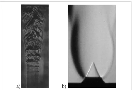
a) b)
Figure 1.1 Schlieren imagery depicting the visible differences between a) a typical turbulent flame and (b) a laminar flame Taken from Eickhoff (1982) and Bouvet (2011) respectfully
The visible differences between laminar and turbulent flames can be seen in Figure 1.1. On the left, the turbulent flame is characterized by its chaotic appearance, whereas the laminar
flame on the right of the image is characterized by its smooth appearance. Laminar and turbulent flame regions can be referred defined with respect to flow velocity, as well as the transition process from laminar to turbulent. According to Law (2006), the transition zone can be represented in terms of Reynolds number, a ratio of inertial forces to viscous forces, at a value of approximately 2300. The laminar regime falls below this value and the turbulent regime lies above it.
1.1.3 Adiabatic Flame Temperature
Adiabatic flame temperature, represented as , is an important factor in the analysis of combustion and flames. In “Combustion Physics” by Law (2006), it is explained as the final temperature attained given the combustion of a uniform mixture with an initial temperature and pressure, in which the mixture achieves chemical equilibrium through an adiabatic, isobaric process. Several factors influence , such as the pressure, the initial temperature and the initial composition of the mixture. The equivalence ratio also has a direct influence on , generally peaking in value close to stoichiometry. As the mixture becomes leaner or richer, the value of will decline mostly due to the losses involved in heating the excess reactants.
1.1.4 Flame Stability
For many reasons, it is desirable to have the ability to keep a flame stationary in space. Having the ability to do so implies that a flow of fresh mixture can be delivered to the combustion site at the exact same rate at which the fuel is being burned. In industrial applications, this typically describes the desired performance within a combustor for continuous and predictable operation (for example, a gas turbine or a furnace). Practically speaking, a perfect and continuously-balanced flame is impossible to accomplish. Furthermore, constant operating conditions can very rarely be guaranteed. According to Law (2006), the purpose of flame stabilization is to supply a means by which a flame can be flexible enough to adjust its location, orientation and configuration in a non-uniform, temporally varying flow field. However, stabilization will not always be possible, and the
domain of unstable systems leads to a discussion of concepts such as flashback and blowoff. For burner-stabilized flames, flashback is a phenomenon in which the velocity of the oncoming mixture has decreased to a level below the burning rate, causing the flame to propagate against the flow of the mixture and back into the tube (which can be quite dangerous). Blowoff describes more or less the opposite scenario, in which the velocity of the unburned fuel mixture increases to a value, lifting the flame off the burner. Initially, as the flame is lifted off the burner from the increased flow of the mixture, the burning rate will also increase since there is less heat lost to the burner rim, creating a higher temperature and faster reaction. However, there is a limit at which point the burning rate cannot be further increased and the lifted flame can no longer be sustained. Evidently, the dynamic balance between flame speed and velocity is achieved between the points of flashback and blowoff. In Figure 1.2, curve 3 represents the state in which flow velocity is higher than the flame speed, annihilating the flame at some elevation above the burner rim.
Figure 1.2 Representation of flashback and blowoff Taken from C.K. Law, Combustion Physics,
Cambridge press (2006, p. 360)
Curve 2 displays the initial state in which flashback is possible, whereas curve 1 is a stronger depiction of the state of flashback, where the velocity of the combustible gas is lower than the burning velocity.
From Williams (1985), a flammability limit of a combustible mixture refers to the composition, temperature or pressure in which the mixture cannot be made to burn. Naturally, the flammability limits of a system involve a lower (LFL) and an upper flammability limit (UFL). The LFL represents the lean limit condition whereas the UFL designates the rich limit condition of the system at a given temperature and pressure. Generally, the flammability limits pertain to the combustion of fuel in air.
Table 1.1 Flammability limits in terms of
equivalence ratio of some common fuel-air mixtures at 1 atm
Taken from C.K. Law, Combustion Physics, Cambridge press (2006, p. 347)
Fuel Lower Flammability Limit Upper Flammability Limit
Hydrogen Carbon Monoxide Methane Propane Benzene Butane 0.10 0.34 0.50 0.56 0.56 0.57 7.14 6.8 1.67 2.7 3.7 2.8
Flame reattachment is a seldom researched phenomenon that describes the reattachment of a lifted flame to the nozzle from which the unburned fuel exits. According to Lee and Chung (2001), flame reattachment is due to a nonlinear decrease in a flame’s liftoff height at a particular balance between propagation speed and flow velocity. This phenomenon may be a function of flow velocity, mass/molar fraction, and nozzle diameter, although the exact conditions for flame reattachment require further investigation. Furthermore, there has been relatively little research in regards to the stabilization of a flame from reattachment.
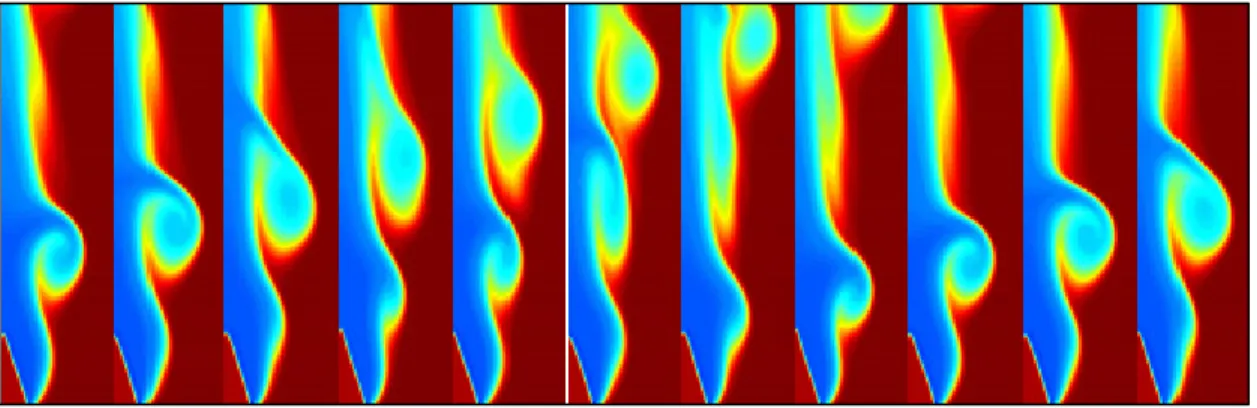
Another flame phenomenon worthy of mention is the occurrence of flame flicker. Shepherd
et al. (2003) describes flame flicker as a buoyancy-driven oscillation, where vortices are
formed due to the interaction of the hot burned gas and the cold ambient air, as seen in Figure 1.3. It is also explained that the frequencies of the flame oscillations can be associated to
several system parameters. In general, the characteristic frequencies of oscillation are in the range of 10 to 20 Hz.
Figure 1.3 Density field representation of vortex evolution over time Taken from Shepherd et al. (2003)
1.2 Laser Spectroscopy
Laser spectroscopic measurement techniques are commonly used in combustion studies. They provide non-obtrusive methods of measuring combustion characteristics in laminar and turbulent flames, such as temperature, density and species concentration. In previous studies, such as Ouimette (2012), laser spectroscopic techniques were successfully used for in-flame measurements of temperature and species concentration. If desired, laser spectroscopy can also be used to measure other characteristics such as velocity flow fields. In this section, the various laser spectroscopic measurement techniques will be examined so as to assess their potential worth to this study.
1.2.1 Raman Spectroscopy
When light is scattered from a light source, the majority of the photons are scattered elastically. Elastic scattering refers to the situation in which the scattered photons maintain the same frequency as the incident photons. However, not all photons are elastically scattered. A very small minority of photons undergoes inelastic scatter; a scenario in which the frequencies of the scattered photons differ from that of the incident photons. When the
scatter is inelastic, it is referred to as Raman scattering since the process is due to the Raman effect. The Raman effect simply refers to the alteration in the wavelength/frequency of light when a light beam is deflected by molecules. This effect was first witnessed by the Indian physicist Sir Chandrasekhara Vankata Raman in 1922.
From Hollas (2004), the frequency (or wavelength) of a photon is related to energy, E, through the Planck relation as seen in Equation ( 1.1 ), where denotes the frequency of the photon, is the wavelength, represents the speed of light and ℎ refers to Planck’s constant:
= ℎ =ℎ ( 1.1 )
This implies that when the frequency or wavelength of a scattered photon differs from that of the incident photon, there is a corresponding change in energy. This corresponding change in energy has been associated with transitions between different vibrational and rotational energy states of the scattering molecule. Typically, Raman applications focus on vibrational transitions due to their larger, more observable shifts. The small rotational shifts generally are not used except when applied to simple gaseous molecules.
The difference in energy between the incident and scattered photons can be demonstrated visually as seen in Figure 1.4:
Figure 1.4 Raman scattering energy level diagram Taken from The Internet Journal of
Vibrational Spectroscopy (2004)
The arrows in Figure 1.4 are of different lengths in order to display the difference in energy between the incident and scattered photons. On the left, the Stokes shift corresponds to a higher final vibrational energy state of the molecule. This means that the scattered photon is shifted to a lower frequency in order for the system’s total energy to remain constant. Conversely, when the final vibrational energy state of the molecule is lower than the inital state, the scattered photon is shifted to a higher frequency. This is illustrated in the right of Figure 1.4 and it is referred to as an Anti-Stokes shift. The Raman shift can be calculated using Equation ( 1.2 ), where λ is the wavelength given in cm and Δ is the Raman shift expressed in wave number, given in cm-1 as explained in Hollas (2004):
Δ = 1 − 1 ( 1.2 )
A normal mode of vibration is a pattern of motion in which the components of a system moving sinusoidically with the same frequency and with a constant phase angle. An object, such as a bridge, a building or a pipeline, has a set of normal modes which depend on several
factors such as the design of the system as well as the materials used. The system can achieve any of its normal modes depending on the conditions set upon it, such as loads, earthquake, wind, etc. A similar concept applies to molecules, where the normal modes of vibration simply refer to the vibrational states of the molecule which depend on the sinusoidal motion of the molecule’s atoms. The molecule can achieve its vibrational states by absorbing or emitting energy due to the interaction of incident photons. Linear molecules with N atoms possess 3N-5 normal modes, whereas non-linear molecules possess 3N-6 normal modes. The vibrational spectrum of a molecule is dependent on its “design”, including the mass and arrangement of each of the molecule’s atoms, which is analogous to the “design” of a structure in the physical world. The vibrational spectrum is therefore unique to each molecule and can be referred to as the “fingerprint”. This implies that if the Raman scattering characteristics of a certain species are known, useful properties and information of the species can be measured. Vibrational spectra are particularly useful in the study of molecular structure. For gases, the combination of rotational and vibrational spectra is useful in the study of combustion reactions.
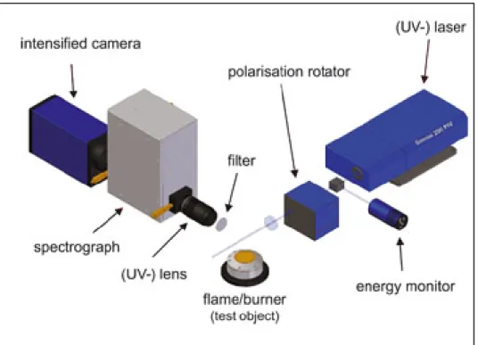
Raman spectroscopy usually involves shining a laser beam onto a sample and collecting the incident light with a lens. This collected light is sent to a monochromator in which the elastic Rayleigh scattering is filtered out. The remaining Raman spectral response provides information about the vibrational modes of the molecules under investigation. This process can be applied to most solid and liquid samples. Gases produce less visible Raman effects due to their relatively low concentrations of molecules (at normal pressures), so special equipment may be required. Typically, a stronger laser is required in order to deliver a more intense beam of light in gaseous applications according to Hollas (2004).
Raman spectroscopy can be applied to the study of mixtures. Each species within a mixture can be observed simultaneously due to each species’ characteristic Raman spectral response. For a given species, the characteristic Raman line pattern will vary in intensity depending on the number of scattering molecules in the mixture sample. The relative concentrations of each species are directly proportional to the relative intensity of each response, which makes
Raman spectroscopy a particularly useful tool in studying species concentrations. Other properties such as density and temperature can be derived by measuring these intensities. Figure 1.5 illustrates the general Raman spectroscopy experimental arrangement suitable for the study of a combustible mixture. A more detailed description of the Raman scattering laser diagnostic setup will follow in Chapter 2.
The major disadvantage of Raman spectroscopy is the weakness of the Raman scattering signal. The signal strength is relatively weak in comparison to that of elastic scatter.
Figure 1.5 An illustration of a Raman spectroscopy experimental setup Taken from LaVision website
1.2.2 Rayleigh Scattering
Rayleigh scattering refers to the elastic scatter encountered during the interaction of an incident photon with a particle much smaller than the wavelength of the light. This scenario applies to gas phase molecules which makes Rayleigh scattering particularly useful for gas applications. The elasticity of the interaction is illustrated in Figure 1.6:
Figure 1.6 Rayleigh scattering energy level diagram Taken from The Internet Journal of
Vibrational Spectroscopy (2004)
The combination of particle size and the wavelength of the incident light determines the extent of Rayleigh scatter for a given light beam. The intensity of scattered light is related to particle size and wavelength in Equation ( 1.3 ). From Hollas (2004):
= 1 + cos 2
2 − 1
− 2 2 ( 1.3 )
The intensity of scattered light due to a single particle is denoted by I, the initial beam of light of wavelength λ is denoted by Io and the scattering angle is θ. The size of the small particle is represented by its diameter d and the distance to the particle is given by R, whereas
n refers to the particle’s refractive index. Equation ( 1.3 ) demonstrates that low-wavelength
(or high-frequency) light is more susceptible to scattering. The blue sky owes its colour to this phenomenon since the shorter blue wavelengths are more intensely scattered than the longer red wavelengths.
Since Rayleigh scattering lacks the Raman shift “fingerprint”, Rayleigh scattering is not useful for determining species concentration. However, if the mole fractions of all major species in a sample are known, Rayleigh scattering can be an effective tool for determining the properties of the sample. Specifically, planar temperature fields can be derived from Rayleigh scattering provided the gas composition is known. The intensity of the Rayleigh signal is much stronger than the Raman signal, which makes Rayleigh spectroscopy a more suitable procedure for determining temperature fields of gases provided the constituent species concentrations are known.
The experimental setup for Rayleigh spectroscopy is usually similar to that of Raman spectroscopy (seen in Figure 1.5). Typically, a laser sends a beam of light onto a sample and the incident light is collected with a lens. However, in this case the Rayleigh scattering is not filtered out from the collected light. Although the similarities in the two experimental approaches makes it simple and natural to utilize combined Raman and Rayleigh techniques.
1.2.3 Laser Induced Fluorescence
Laser induced fluorescence (LIF) involves the excitation of a sample’s molecules to higher energy levels through the absorption of photons (typically from a laser beam). Some of these molecules fluoresce by de-exciting and emitting photons at a wavelength longer than the incident light’s wavelength. The level of fluorescence is dependent on the species concentration as well as the temperature and pressure of the sample. The emitted fluorescent light is usually captured by a photomultiplier tube. The excitation light can be filtered out since it is of a different frequency than the fluoresced light.
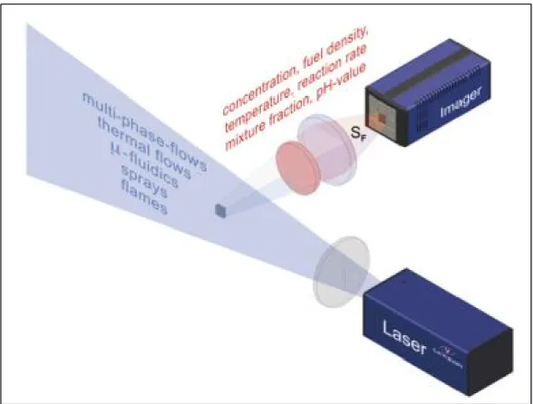
LIF imaging usually involves a procedure referred to as planar laser induced fluorescence (PLIF). Typically, PLIF uses a pulsed laser beam as a light source. The beam of light from the laser is usually fed through an arrangement of lenses and/or mirrors and emerges as a sheet of light which illuminates the fluid of interest. The resulting fluorescence is delivered through a filter and captured by a camera. If the fluid is not composed of a fluorescent
substance, the flow can be seeded with a fluorescent marker or tracer. An advantage of PLIF is that many combustion fuel species can be visualized directly without the need of markers or tracers. PLIF enables the determination of several flow variables, some of which include temperature, density, pressure and velocity. It is also known to have a high sensitivity in comparison to Rayleigh and Raman techniques, having the ability to detect species at the ppm level. Figure 1.7 illustrates a typical PLIF experimental setup.
Figure 1.7 An illustration of a typical planar laser induced fluorescence experimental setup. Taken from the LaVision website
1.3 Laminar Flame Speed
The design of combustion engines cannot be accomplished without a thorough grasp of the laminar flame speeds of combustible gases. Laminar flame speed describes the propagation speed of an unstretched laminar flame. The term is often used interchangeably with “laminar burning velocity”, although they differ slightly in meaning; laminar burning velocity refers
specifically to the property of a combustible mixture that describes the velocity of the combustion reaction relative to the unburned gas. Although there still remain several questions surrounding the structure of propagating laminar flames, equations do exist for use in theoretical analyses.
When Mallard and le Chatelier initially studied deflagration, it was believed that heat loss was the central factor affecting the propagation of laminar flames. The rates of chemical reactions were thought to affect these speeds to a lesser extent. According to Williams (1985), it was Mikhel’son who demonstrated that the burning velocity is proportional to the square root of the reaction rate as well as the square root of the ratio of the thermal conductivity to the specific heat at constant pressure. More recently, the development of asymptotic concepts within the scope of laminar flame theory has helped improve the accuracy with which burning velocity is calculated.
The influence of initial pressure on laminar flame speed is a topic of interest in combustion research. As initial pressures increase, it has been shown that laminar burning velocities decrease. This phenomenon is evident in Hu et al. (2009) as demonstrated both experimentally and numerically with hydrogen-air mixture. However, it was also demonstrated that an increase in initial pressure induces cellular instability and ultimately leads to an increase in flame instability. Tse et al. (2000) conducted a separate study to further examine the effects of pressures up to 60 atm on hydrogen flame propagation. Using the combustion bomb method (see Section 1.3.2), Law witnessed the flame instability at high initial pressures lead to the onset of heavy wrinkling on the flame surface at as low as 5 atm. This observation has particular significance because it reveals how the assumption of a smooth flame can be very misleading. The flame may appear to decrease in propagation rate as initial pressure increase. However, the heavy wrinkling increases the surface area over which the chemical reactions are taking place, resulting in a faster burning rate than had been originally observed. Law suggests that the flame may simply be trying to respond to the increase in pressure by creating wrinkles to maintain a higher burning rate. Note that this fundamental discovery in no way states that an increase in initial pressure results in an
increase in flame speed, but it opens the door to new research objectives. As well, this is yet another example of why it is important to visually record the deflagration.
Conversely, initial temperature conditions have shown little effect on flame stability. Nevertheless, an increase in initial temperature has shown to produce an increase in unstretched flame propagation as well as unstretched laminar burning velocity in Tang et al. (2008).
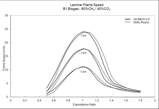
The influence of equivalence ratio on laminar flame speed can be partially investigated by analyzing its effect on flame temperature, although this does not apply to very rich mixtures in which case flame speed becomes increasingly limited by the rate of diffusion. Due to the heat of combustion and heat capacity of reaction products, it is a well-known phenomenon that maximum flame temperatures are found at slightly rich equivalence ratios, as stated by Tse et al. (2000). Consequently, the maximum flame temperature generally corresponds to the maximum laminar flame speed for combustible gases. Over a range of different equivalence ratios, one could expect a bell-curve-shaped graph in which the maximum lies slightly above = 1. An example of the typical relationship between laminar flame speed and equivalence ratio can be seen in Figure 1.8, which has been lifted from Appendix IV. It is worthwhile to note that the opposite relationship describes the laminar flame thickness with respect to equivalence ratio. As demonstrated by Tang et al. (2008) for a propane-hydrogen-air mixture, the relationship produced a U-shaped curve in which the minimum flame thickness was found around stoichiometry. Once again, this relationship does not apply to very rich mixtures.
Figure 1.8 Example of the typical relationship between laminar flame speed and equivalence ratio at varying pressure
Another important consideration in laminar flame speed experimentation is the fuel type. Alkanes (such as methane, ethane and propane) are generally known for having lower laminar flame speeds. Alkenes (such as ethylene) generally have slightly faster burning velocities and reach higher flame temperatures at laminar flame speed, whereas alkynes burn faster still. The simplest of all fuels, hydrogen, is known for being reactive and possessing a very high burning velocity. Based on the findings of Tang et al. (2008), it can be expected that an increase in hydrogen percentage will render the mixture more reactive and thus increase the laminar flame speed. This explains hydrogen’s presence in so many combustible gas mixtures. Not only does hydrogen have high thermal and mass diffusivity, but it also lacks the reaction of carbon monoxide to carbon dioxide present in hydrocarbon reactions. Monteiro et al. (2010) presents a comprehensive account of laminar burning velocities for various syngas mixtures.
Researchers have developed several different methods of experimentally measuring laminar flame speed, each method with its own level of uncertainty. The main techniques and their derivatives as observed in the literature will be described. The three main approaches to be discussed here are the Bunsen flame method, the combustion bomb method, and the stagnation flame method.
1.3.1 Bunsen Flame Method
The Bunsen flame method is a popular approach to determining laminar flame speed. Typically, this approach involves a premixed mixture flowing with a velocity v through a cylinder of diameter d. The air-fuel mixture produces a conical, fuel-rich inner flame surrounded by a diffusion flame. When the flame is stable, both the premixed and diffusion flames remain stationary. Although it has been shown by Echekki and Mungal (1991) that the flame speed is not constant over the entire flame surface, the Bunsen flame technique remains a popular method of determining laminar flame speed due to the simplicity of the experimental procedure. Perhaps the most significant drawback of this method is that it overlooks the influence of stretch on the flame speed measurements. Although the accuracy of the Bunsen flame method has been questioned, critical analyses have shown that it can produce results of sufficient accuracy.
As the gaseous mixture exits the burner, the normal of unburned gas velocity is equivalent to the flame speed for perfectly stationary flames. This is the principle behind the flame angle method. As seen in Figure 1.9, by measuring the angle ∝ between the premixed flame edge and the direction of the unburned gas velocity vu, the flame speed S is equal to the normalized
unburned gas velocity, , , and can be easily calculated according to Equation ( 1.4 ):
Figure 1.9 Bunsen burner apparatus depicting the angle between the premixed flame edge and the unburned gas velocity Taken from C.K. Law, Combustion Physics, Cambridge press (2006, p. 264)
In this approach, burners with contoured nozzles are generally favoured since they attempt to neutralize boundary layer effects. These boundary layer effects cause straight cylindrical burners to produce parabolic exit velocity profiles, which in turn causes premixed flames to be parabolic in shape as well. Contoured nozzles result in stabilized flames that are more conical in shape. This provides straighter edges with which to measure the flame’s half cone angle α, but it does not guarantee straight edges. In Bouvet et al. (2011), contoured nozzle burners were utilized in determining the laminar flame speeds of a range of syngas mixtures composed of H2/CO/Air. Despite the varying gas flow rates, it was observed that the contoured nozzles failed to produce straight-sided conical flames under each of the scenarios examined. The data from the flame angle method was used to compare with results obtained from another popular Bunsen flame approach called the flame area method, also under investigation by Bouvet et al. (2011) in the same study. In the flame area method, the
average laminar flame speed is calculated by dividing the gas flow rate by the surface area of the flame. If and are respectively the mass and volume flow rates of the unburned gas, is the unburned gas density and is the flame surface areas, then the conservation of mass states in Equation ( 1.5 ):
= ( 1.5 )
= = ( 1.6 )
Since Equation ( 1.6 ) divides the gas flow rate over the surface area of the flame, there is an inherent assumption that the flame speed is constant over the entire surface area of the flame. As stated earlier, the flame speed is not constant over the surface area of the flame, meaning the flame area method does not calculate the true laminar flame speed . Equation ( 1.6 ) solves for an averaged flame speed S that can closely approximate when utilized carefully. It is common for direct imaging techniques to successfully capture the flame edges. Schlieren or shadow photography tend to produce flame images with enhanced flame edge clarity. Traditionally, the inner edge of shadowgraph imagery has provided the best results due to its proximity to the unburned flame surface. Another valid technique involves tracing the flame edge by recording the maximum OH* chemiluminescence emission. In Bouvet et al. (2011), the OH* chemiluminescence methodology was even preferred over Schlieren diagnostics since it provided results comparable to the literature without the use of complex tracking techniques.
Although the flame angle and flame area approach appear quite straightforward due to the simplicity of Equations ( 1.5 ) and ( 1.6 ), they encounter complications in other areas. Due to the large difference in temperature between the flame and the burner rim, there is always a heat loss to the rim which reduces the flame speed. As well, with smaller diameter burners, the calculated flame speed increases approaching the flame tip when using Equation ( 1.4 ). This is due to the flame’s curvature at the apex of the cone. As the flame edge approaches the
centerline, α approaches 90° and in turn, S approaches . Since the flame surface does not produce a perfect cone, surface identification is difficult and stretch effects often go unaccounted for. This inconvenience can be eluded by using a flat-flame burner, reducing the 2-dimensional Bunsen flame to a 1-dimensional flat flame. This planar flame is normal to the unburned gas flow direction. The surface area of the flame is easily and accurately defined which reduces the potential for error. Applying Equation ( 1.6 ) produces the laminar flame speed. However, the flat-flame burner is non-adiabatic. The flat, porous burner has a cooled surface on which the flat flame is stabilized. Although this method eliminates the problem of stretch due to curvature, it yields a burning velocity lower than the true unstretched burning velocity ( ) due to heat loss at the burner surface. In spite of this, measurements can be corrected for heat loss by varying the gas flow and tracking the corresponding cooling rate, then extrapolating the cooling rate to zero as explained in Law (2006).
1.3.2 Combustion Bomb Method
This method involves measuring a spherically expanding flame kernel in a combustion bomb ignited at the center of the combustion chamber. Rallis and Garforth (1980) concluded in their study that the spherical constant-volume combustion bomb method is the most versatile and accurate for experimentally determining the laminar flame speed. Typically, combustion chambers for this purpose are spherical in order to complement the flame’s assumed spherical shape. The flame’s spherical shape should nonetheless be verified visually upon experimentation if this method is to be used.
The flame propagates outward at the combustible mixture’s laminar flame speed, thus the point of ignition is purposely located at the center of the chamber to allow for maximum propagation before disturbance from the chamber walls. As the deflagration wave spreads, the total amount of products from the reaction increases and the chamber pressure increases accordingly. Furthermore, the unburned gas upstream of the propagating flame is compressed, which in turns heats the unburned gas. As the unburned gas is subjected to higher pressures and temperatures, the initial state no longer applies within the confines of
the chamber. The combustion bomb experiment must therefore take this into account by measuring the pressure and temperature of the unburned gas over the course of the deflagration. Another option is to limit data acquisition to the time period in which the flame size is relatively small. In doing so, the pressure and temperature upstream of the flame should approximate the initial state to the point where the difference can be discounted. However, by limiting the data acquisition period to a smaller time window, the need for strong acquisition tools becomes more significant. Luckily, thanks to the increased use of better data acquisition systems, many of the problems inherent to the combustion bomb method have been overcome over the years or have been proven to be insignificant, according to Rallis and Garforth (1980).
The best option in laminar flame experimentation is to record the deflagration with a high speed photography system. This is the most direct way of documenting the history of the flame’s spherical expansion. The rate of change of this radius is thus the flame propagation rate. This procedure requires optical windows within the chamber to record the flame progression. Commonly, the windows on such chambers are diametrically opposed and made of quartz, which can withstand high pressures and temperatures. It is best to include pressure and temperature sensors to monitor the state of the unburned combustible mixture. According to Gu et al. (2000), once significant pressure variation has commenced within the chamber, a pressure-time curve can be used to calculate the laminar flame speed. This makes it possible to cross-reference the calculated flame speed values with the observed values from the photography, as originally done by Manton et al. (1953). As well, if a high speed photography system cannot be obtained, the pressure history can serve as the single experimental input. The cube-root-law has been the most recognized model applied to a pressure-time curve in order to estimate the burning velocity and flame thickness.
The calculation of laminar flame speed from the pressure-time curve does come with its drawbacks. Since the pressure variations are more significant once the flame is relatively large, more time has passed for other outside factors to affect the deflagration, such as buoyancy. The deflagration is not homogeneous, meaning the reaction does not occur
uniformly throughout the vessel. Instead, the quantity of hot products increases and the quantity of cold reactants decreases as the flame propagates. This presence of hot products and cold reactants causes the spherical shape of the flame to adjust to more of a mushroom shape, according to Dahoe and de Goey (2003). Naturally, at lower burning speeds, buoyancy will be expected to introduce a greater degree of error. Evidently, it is risky to rely solely on the pressure-time curve as experimental input. The experiment can always be limited to the early portion of the pressure-time curve where it is safer to assume that the flame is spherical in shape, but pressure variations are less significant over this period so it can be problematic trying to determine which segment of data to use. A high-speed photography apparatus should be included within the experimental setup at least to verify the validity of the flame’s spherical shape over time. At worst, if the spherical propagation of the flame tends to lose its shape, approximate corrections can be introduced as was done by Rallis and Garforth (1980).
The assumption is often made that there is no heat loss or gain from the burned or unburned regions. However, heat transfer is possible in several manners. For instance, heat may be transferred from the burned gas to the unburned gas, from the unburned gas to the walls of the chamber and also from the burned gas to the centrally positioned ignition system (particularly during the initial propagation phase). Heat transfer by radiation is also possible from the burned or unburned gases to the chamber walls, according to Rallis and Garforth (1980), who was able to show that heat transfer does occur but its effect is minimal. Generally, it is important to note that heat losses that reduce the flame temperature will also reduce the flame speed.
Since the pressure and temperature values change simultaneously within the chamber, correlations are required to account for their influence. These correlations offer an approach to circumventing the assumption that downstream pressure and temperature states at any instant are uniform throughout the unburned gas. Many correlations have been proposed over the years, many of which account for the temperature gradient downstream of the flame. This section will not cover the various correlations. Instead, it is simply important to note that
there exist correlations covering the influence of a wide range of unburned gas conditions. Parameters such as pressure, temperature and equivalence ratio can be simultaneously related to laminar flame speed for different fuel types. Each correlation comes with a certain degree of error and should only be used over the specified range.
1.3.3 Stagnation Flame Method
The stagnation flame method, sometimes referred to as the counterflow or twin flame method, involves the projection of two identical gas flows upon each other. This creates a “stagnation plane” at the location of collision. Igniting the system produces two symmetrical flat flames, each one located equidistantly on either side of the stagnation plane. Figure 1.10 depicts the stagnation plane and twin flame arrangement.
Figure 1.10 Depiction of the twin flames in the stagnation flamemethod
In order to utilize this phenomenon for measurement purposes, it is necessary to understand the behaviour of the normal velocity component v with respect to the distance from the stagnation plane. As the gas flow approaches the stagnation plane prior to the preheat zone, the normal velocity decreases linearly according to Equation ( 1.7 ), where is the velocity gradient as well as the stretch rate (s-1) which is calculated in Equation ( 1.8 ):
= ( 1.7 )
= ( 1.8 )
Entering the preheat zone, the increase in heat causes v to increase. In Figure 1.11, this decreasing trend is illustrated until , after which point increases linearly. At , the increasing trend is once again reversed as the heat release is terminating and approaches the stagnation flame. The and represent reference flame speeds at the upstream boundary of the preheat zone and the downstream boundary of the reaction zone respectively. In order to eliminate the stretch effect, can be plotted against and extrapolated to
= 0. The laminar burning velocity is simply equal to at this intercept. Since is used as the reference flame speed, the calculated laminar burning velocity represents assessed at the upstream boundary. According to Law (2006), is typically evaluated at the upstream boundary because heat loss and flow nonuniformity effects are minimized.
Figure 1.11 Axial profile illustrating the normal velocity of the gas flow with respect to the distance from the stagnation plane
Taken from C.K. Law, Combustion Physics, Cambridge press (2006, p. 272)
1.4 Previous Works
This section contains a review of the studies conducted by other researchers that are similar in execution and/or subject matter to this project. At the time of this writing, there appears to be no available documentation of studies involving laser diagnostic techniques as a means to investigate flame structure of partially premixed laminar flames of H2/CO/CO2 or H2/CO/CH4/CO2 mixtures. The majority of research conducted on partially premixed laminar flames of such mixtures concerns the measurement of laminar flame speed.
1.4.1 Flame Structure
Fernández et al (2006) studied lean, premixed CH4/air laminar flames using Bunsen burner to stabilize the flames. The concentrations of the major species present in the flame as well as the flame temperature were measured using Raman spectroscopy. The objective of this study was to validate that Raman spectroscopy is an unobtrusive measurement technique that can be used to measure local properties in stationary flames. Experimental results from this study compared quite favourably with the literature.
Rabenstein and Leipertz (1998) used Raman spectroscopy to measure the major species concentrations (CH4, H2, H2O, CO2, N2 and O2) and temperatures of rich, partially premixed CH4/air flames. The experimental measurements were obtained at various elevations above the exit of a dual flow burner, upon which the flame was stabilized. The results of the investigation concluded that the reaction zone can by identified by a region in which the unburned, premixed gas constituents decrease in concentration. This observation was coupled with an increase in molar fraction of the CO2 and H2O, which in this case represented the products of combustion. It was further shown that the boundary of the reaction zone is characterized by the diffusion of ambient air into the flame, which appeared in the Raman results as an increase in concentration of O2 and N2. This boundary was also represented in the temperature measurements, seeing as the temperature gradually reduced to ambient value towards the flame’s periphery. As the elevation of the measurement increased with respect to the flame’s height, this reaction zone boundary visibly shifted in the radial direction from the flame’s central axis. The conclusion of this study was thus that Raman spectroscopy adequately provides a means of quantifying flame structure.
Han et al. (2006) studied the structure of low-stretch methane nonpremixed flames both experimentally and numerically. The objective of the study was to analyse the effects of flame radiation on flame response and extinction limits. The experimental setup involved generating a CH4/N2 flame using a porous, spherically symmetric burner with a large radius of curvature. Gas and flame temperatures were measure by Raman scattering while the temperature of the burner surface was measured by IR imaging. Furthermore, the reaction zone boundaries were illustrated through OH-PLIF and chemiluminescence imaging. The numerical investigation simulated low-stretch flame structure by accounting for detailed chemistry, thermodynamic/transport properties as well as radiative aspects. The study concluded with an agreement between the numerical results and the experimental observations.
Cheng et al. (2011) undertook an experimental and numerical investigation to characterize laminar premixed H2/CO/CH4/air flames at atmospheric conditions. The objective of the
study was to determine the effects of varying the fuel composition on the resulting flame characteristics at fixed stoichiometry. The experimental measurements were performed using an opposed-jet burner technique, which is described in Section 1.3.3 (stagnation flame method). The temperature and flame front position are measured and compared to results obtained from EQUIL and PREMIX numerical flame simulations. Flame structure was simulated using the OPPDIF package with the GRI Mech 3.0 mechanism. Cheng et al. (2011) concluded that the experimental measurements of flame front position and temperature were closely predicted by the simulations from the CHEMKIN codes. Furthermore, the chemical kinetic structures indicated that the increase in laminar flame speed associated with H2 addition is probably owing to chemical effects as opposed to thermal effects.
1.4.2 CO2 Dilution
Natarajan et al. (2007) studied the effect of CO2 dilution on laminar flame speed on lean H2/CO mixtures. The study covered a range of fuel compositions and CO2 dilution levels and used a Bunsen flame approach, measuring the flame speed from images of the reaction zone area. The experimental results were compared to numerically simulated results; experimental data was compared to the GRI Mech 3.0 and Davis H2/CO mechanisms, of which the Davis mechanism compared more favourably, particularly at higher H2 concentrations. The study reports that flame speed decreases with increased CO2 dilution due to the capability of CO2 to lower the flame temperature by way of radiative heat transfer. More specifically, the CO2 in the unburned fuel absorbs radiative energy from the hot products such as CO2 and H2O. The study concludes that the prediction models accurately predict the flame temperature and chemical effects related to CO2 dilution.
Park et al. (2008) conducted a numerical study of H2/CO syngas diffusion flames diluted with CO2. The objective of the study was to gain further insight into the influence of fuel composition and flame radiation on flame structure and the oxidation process. The numerical results were compared to the models of Sun et al. and David et al., seeing as these models
were considered leaders in H2/CO flame modelling. The investigation shows that losses in flame temperature are due to radiation increase as CO and CO2 mole fractions increase. It was also demonstrated that H2 and CO oxidation reaction pathways are sensitive to H2/CO composition as well as the addition of CO2.
An investigation of laminar burning velocities and flame stability was conducted by Burbano
et al. (2011) for equimolar H2/CO mixtures with dilution of two separate inert gases, CO2
and N2, at ambient conditions. Premixed laminar flames were produced using a contoured, slot-type burner and the angle method was used to calculate laminar flame speed from Schlieren imagery. The experimental measurements were compared to numerically computed results from three reaction mechanisms: Frassoldati et al., Davis et al., and the H2/CO/O2 reactions of Li et al. The study concluded that N2 and CO2 dilution lowers the laminar burning velocity of the mixture due to the decrease in heat release and the increase in heat capacity. Between the two diluents, the effect was larger in the case of the CO2 diluent due to its dissociation during combustion as well as its greater heat capacity. Burbano et al. observed flame instabilities at lean conditions and that H2 has the tendency to destabilize the flame. On the other hand, CO has a stabilizing effect on the flame by decreasing hydrodynamic and thermal-diffusive instabilities. In the end, the destabilizing effect of H2 is more dominant. When either of the two diluents is added to the mixture, instabilities were observed over a wider range of equivalence ratios, although stable flames are more likely to be obtained at rich equivalent ratios.
1.4.3 Biogas with CO2 Dilution
An experimental study conducted by Cohe et al. (2009) investigated laminar and turbulent lean premixed CH4/CO2/air flames at various pressures using Bunsen flame. The investigation involved the analysis of flame propagation speed, flame surface density as well as wrinkling parameters of the flame front. The experimental data and PREMIX computations both revealed that CO2 addition decreases the laminar flame speed.