Document de travail (Docweb) nº 1305
Development at the border: policies and national
integration in Côte d’Ivoire and its neighbors
Denis Cogneau
Sandrine Mesplé-Somps
Development at the border: policies and national integration in Côte d’Ivoire
and its neighbors
Abstract: By applying regression discontinuity designs to a set of household surveys from the
1980–90s, we examine whether Côte d’Ivoire’s aggregate wealth was translated at the borders of neighboring countries. At the border of Ghana and at the end of the 1980s, large discontinuities are detected for consumption, child stunting, and access to electricity and safe water. Border discontinuities in consumption can be explained by differences in cash crop policies (cocoa and coffee). When these policies converged in the 1990s, the only differences that persisted were those in rural facilities. In the North, cash crop (cotton) income again made a difference for consumption and nutrition (the case of Mali). On the one hand, large differences in welfare can hold at the borders dividing African countries despite their assumed porosity. On the other hand, border discontinuities seem to reflect the impact of reversible public policies rather than intangible institutional traits.
Keywords: National Integration, Africa, Borders, Economic Geography, Welfare JEL Classification: O12, R12, P52
Résumé: En appliquant plusieurs méthodes de régressions par discontinuité à un ensemble
d'enquêtes auprès des ménages pour les années 1980 et 1990, nous examinons si la richesse macro-économique de la Côte d'Ivoire se constatait aux frontières avec les pays voisins. A la frontière du Ghana et à la fin des années 1980, de larges discontinuités sont détectées en matière de consommation, de retard de croissance infantile, et d'accès à l'électricité ou à l'eau. Les discontinuités frontalières de consommation peuvent être expliquées par les différences de politiques concernant les cultures d'exportation (café et cacao). Quand ces politiques ont convergé dans les années 1990, seules les différences d'infrastructures rurales ont persisté. Dans le Nord, le revenu des cultures d'exportation (coton) engendrait aussi une différence en matière de consommation et de nutrition (cas du Mali). D'un côté, de larges différences de bien-être peuvent s'observer aux frontières divisant des pays africains, malgré leur supposée porosité. D'un autre côté, les discontinuités frontalières semblent refléter l'impact de politiques publiques réversibles, plutôt que des caractéristiques institutionnelles intangibles.
Development at the border: policies and national
integration in Cˆ
ote d’Ivoire and its neighbors
Denis Cogneau, Sandrine Mespl´
e-Somps and Gilles Spielvogel
∗Abstract
By applying regression discontinuity designs to a set of household surveys from the 1980–90s, we examine whether Cˆote d’Ivoire’s aggregate wealth was translated at the borders of neighboring countries. At the border of Ghana and at the end of the 1980s, large discontinuities are detected for consumption, child stunting, and access to electricity and safe water. Border discontinuities in consumption can be explained by differences in cash crop policies (cocoa and coffee). When these policies converged in the 1990s, the only differences that persisted were those in rural facilities. In the North, cash crop (cotton) income again made a difference for consumption and nutrition (the case of Mali). On the one hand, large differences in welfare can hold at the borders dividing African countries despite their assumed porosity. On the other hand, border discontinuities seem to reflect the impact of reversible public policies rather than intangible institutional traits.
Keywords: National Integration, Africa, Borders, Economic Geography, Welfare. JEL classification codes: O12, R12, P52
∗Denis Cogneau (corresponding author) is senior research fellow and associate professor at Paris School of Economics - IRD; his e-mail address is [email protected]. Sandrine Mespl´e-Somps is research fellow at Institut de Recherche pour le D´eveloppement (IRD), UMR 225 DIAL, Universit´e Paris Dauphine; her e-mail address is [email protected]. Gilles Spielvogel is assistant professor at Universit´e Paris 1 Panth´eon-Sorbonne, UMR 201 “D´eveloppement et Soci´et´es” (Universit´e Paris 1 - IRD), and DIAL; his e-mail address is [email protected]. The authors thank the National Institutes for Statistics of Cˆote d’Ivoire, Ghana, Guinea, Mali, and also Burkina Faso, for giving access to their survey data. They thank Charlotte Gu´enard and Constance Torelli for their participation in the first stage of this study; for historical archives, excellent research assistance from Marie Bourdaud and Ang´elique Roblin is gratefully acknowledged. They last thank seminar participants at Oxford (CSAE), The Hague (ISS), Clermont-Ferrand (CERDI), Paris (CEPR/EUDN/AFD Conference and PSE), and Washington (World Bank), as well as three anonymous referees. The usual disclaimer applies.
State consolidation is widely considered to be the most important issue for the development of Africa (e.g., Levy and Sahr Kpundeh 2004), and State failure is of-ten related to difficulties presented by artificial international boundaries (Alesina, Easterly, and Matuszevski 2012). Some authors even consider redrawing interna-tional boundaries to be a serious option (e.g., Englebert 2000, 181-189, Herbst 2000, 262-269). For the most part, these boundaries were fixed by European colo-nial powers and arbitrarily delineated (Barbour 1961 and other references cited in Englebert, Tarango, and Carter 2002), and they have rarely been modified since then (Brownlie 1979). Given the weakness of African States, the reach of national policies in peripheral border areas has been extensively questioned. Furthermore, African borders are often assumed to be permeable, particularly to informal trade and migration flows that may level international differences. Are African bound-aries still abstract lines drawn on a map, so that divided areas remain alike and no difference in welfare is observed when crossing the border? Or have they become real,strong discontinuities that reveal an ongoing process of national integration? These are the questions that we address in this paper.
The literature on Africa’s development presents a variety of arguments regard-ing the role played by boundaries between States.
A first group of contributions supports the idea of boundaries’ weaknesses and porosity. This idea is implicitly present in papers stressing the role of geography (e.g., Bloom and Sachs 1998). Other papers more directly build upon the under-development of state institutions. According to Herbst (2000, 171), the guaranty from the United Nations discourages African States from investing in territorial control; whoever holds the capital city holds the country, “the broadcast of power radiating out [from the political core] with decreasing authority”. These
“territory-states”, as opposed to nation-states, are in keeping with pre-colonial political in-stitutions in a context of low population density. Within former French West Africa, Huillery (2009) relates part of the present-day spatial inequality within countries to decentralized policies in early colonial times. Other papers propose the role of ethnicity. Common languages and cultures contribute to informal cross-border flows of goods, money, and people across “permeable boundaries” (Griffiths 1996). Studying the markets for millet and cowpea at the Niger-Nigeria border, Aker et al. (2010, 26) argue that “ethnic borders map the geography of trade more effectively than international borders do”. According to Michalopoulos and Papaionnou (2012, 2013), in Africa, precolonial political institutions are a more powerful determinant of development than national institutions. At the border between Cˆote d’Ivoire and Ghana, Bubb (2012) finds no difference in the man-agement of property rights on land. Finally, Easterly and Levine (1998) find that countries’ growth is strongly influenced by the countries’ neighbors.
A second strand of the literature stresses the salience of national idiosyncrasies and a centripetal effect of boundaries. As noted by Robinson (2002) in his review of Herbst, the boundaries of Latin American countries, which became indepen-dent at the beginning of the 19th century and are now considered well-established nation-states, also exhibit some degree of arbitrariness. Bach (2007) presents a similar argument. Furthermore, ethnic salience is not fate. Posner (2004) observes that among two ethnic groups at the border between Malawi and Zambia, ethnic identification varies when crossing the border. Miguel (2004) suggests that the promotion of national identity by the Tanzanian leader Julius Nyerere succeeded in canceling out the negative impact of within-village ethnic heterogeneity on pub-lic goods provision observed in neighboring villages of Kenya. Furthermore, many
authors emphasize that differences in prices, taxes, and market demand create eco-nomic opportunities that are exploited every day by agents living in border areas (Bach 1997, Nugent 2002). Although initially arbitrarily delineated, boundaries have become a reality, if only for economic life. Comparing communities on both sides of the Cˆote d’Ivoire-Ghana border, MacLean (2010) argues that patterns of social insurance differ and were shaped by colonial and post-colonial state action. Asiwaju (1976) and Miles (1994) develop similar arguments about the contrast between British and French colonial imprints at the Benin-Nigeria and the Niger-Nigeria borders, respectively. Finally, at the macroeconomic level, the inequality of income between African countries is larger than usually thought. According to Schultz (1998), the log variance of GDP per capita in PPP reached 0.415 in 1989 in Africa (including North Africa), which is by far the highest level of all regions of the world. Furthermore, this number is twice as high as it was in 1960 (0.213). Of course, income divergence between African countries may only reflect the di-vergence of their centers rather than their border areas. However, this possibility would be difficult to reconcile with a strong influence of neighbors on growth.1
Drawing from a large set of household surveys covering the 1986–98 period, we estimate regression discontinuity designs at the borders of Cˆote d’Ivoire with Ghana, Mali, and Guinea, focusing on four welfare outcomes: consumption and children’s nutritional status (height-for-age), on the one hand, and the connection to electricity and access to safe water, on the other hand. When discussing the main results, we also examine household cash crop output and incomes.
1The insulating power of boundaries is not necessarily for the good. Englebert, Tarango, and
Carter (2002) talk of political “dismemberment” and “suffocation”. Further, the “balkanization” of Africa is often believed to prevent the exploitation of returns to scale, despite efforts of regional trade integration. However, the impact of full political integration is different from a simple size merger (Spolaore and Wacziarg 2005).
Cˆote d’Ivoire is an interesting case study; at least in the 1980s and 1990s, it was much wealthier than all of its neighbors. The evidence provided by border discontinuity estimates is more mixed.
We document the hazards that commanded the alignment of boundaries during the colonial era and show that predetermined geographical and historical condi-tions should not account for border discontinuities in welfare.
At the eastern border with Ghana and at the end of the 1980s, large border discontinuities existed for the four outcomes. However, because the 1990s brought crisis to Cˆote d’Ivoire and recovery in Ghana, border differences in income were very much attenuated, and the discontinuity in nutrition vanished. Discontinuities in access to electricity and water were preserved. In contrast, at the northern bor-der with poorer and landlocked Mali and in the mid-1990s, Cˆote d’Ivoire performed better in terms of income and nutrition, but not in access to utilities. The border with Guinea provides a case in which the Cˆote d’Ivoire advantage is canceled out along all dimensions. A more detailed analysis shows that income derived from cash crops almost fully accounts for the large differences in consumption at the borders of Ghana and Mali. Because the cocoa frontier had not yet reached the extreme west in the 1990s, the same factor explains why no discontinuity is found at the border with Guinea.
Border discontinuities reveal the role of two types of national policies: policies affecting cash crop production and public investment in utilities. Although differ-ences in such policies have had large and visible impacts at borders, they are not irreversible, and some of them were changed in the years that followed. We con-clude that large border discontinuities can be observed between African countries in the short run, but they do not necessarily reflect divergent trajectories linked
to long-lasting institutional features.
Section I presents the analytical methodology and explains the econometrics. Section II documents the historical and geographical backgrounds of borders. Sec-tion III presents survey data and border discontinuities in development outcomes, first for the eastern border with Ghana and then for the northern borders. Sec-tion IV provides further discussion of the cash crop channel and naSec-tional policies. Section V concludes.
I.
Analytical methodology
Here, we discuss the conditions under which the borders we study can be considered historical “natural experiments”. Consider a person born somewhere in the area now named Cˆote d’Ivoire. What would her welfare be if Cˆote d’Ivoire had been colonized by the British instead of the French, like Ghana, and then exposed to post-colonial Ghanian policies and institutions? This question is difficult to answer for at least three reasons: (i) the British could have established different institutions to rule Cˆote d’Ivoire; (ii) Ghana and Cˆote d’Ivoire combined would not be the same, if only because of market size and general equilibrium considerations; and (iii) even if Ghana’s institutions had remained the same, we have no idea how Cˆote d’Ivoire’s initial characteristics would interact with them. Now, take a person born in Cˆote d’Ivoire at the border of Ghana and imagine that the border was some kilometers farther. Including this person in Ghana would have a marginal and insignificant impact on Ghana’s institutions and economy. Furthermore, it is very probable that this close neighbor of actual Ghanaian people would share the same geographical constraints and the same precolonial initial conditions.
Let Y be some outcome variable (income, connection to electricity, etc.) ob-served over a sample of people living in two countries at the same date. Let
C = 0, 1 be the dummy variable indicating the country of residence. Let Yi(0)
be the outcome if and when the individual (or household) i lives in the country
C = 0 and Yi(1) in the country C = 1. The observed outcome reads thus:
Yi = (1− Ci).Yi(0) + Ci.Yi(1). (1)
The identification of the average treatment effect, E[Y (1)− Y (0)], is probably out of reach, but a regression discontinuity (RD) design based on distance to the border should correctly approach its local version (LATE) in the vicinity of the border.
Required assumptions for a border RD
Let Di stand for the distance to the border of the locality of residence, positively
signed for country 1 and negatively signed for country 0, so that Ci = 1{Di ≥ 0}.
Under the assumption that E[Y (0)|D = d] and E[Y (1)|D = d] are continuous in d, limd→0+E[Y|D = d] − limd→0−E[Y|D = d] provides an estimation of the average treatment effect at the border (Hahn, Todd, Van Der Klauw 2001). It is the so-called “sharp” RD estimator. As Lee (2008) argues in another context, this continuity assumption is difficult to assess and impossible to test. Lee’s reformula-tion elucidates the condireformula-tions under which an RD replicates a random assignment around the threshold D = 0. Assume Y is generated by a partially unobservable random variable W : Y (0) = y0(W ) and Y (1) = y1(W ). W represents the “type”
stand for the cdf of D conditional on W . Lee’s conditions are as follows (Lee 2008, 679):
(i) F (d|w) is such that 0 < F (0|w) < 1
(ii) F (d|w) is continuously differentiable in d at d = 0, for each w in the support of W
Condition (i) of overlap requires that D can be written D = Z(W ) + e, where
Z is the predictable component of D and e is an exogenous random chance
compo-nent, so that the probability of receiving treatment is somewhere between 0 and 1 for each type. Condition (ii) of unconfoundedness implies that conditional density
f (d|w) is continuous in d at d = 0. In our case, this implies that within each
type w and very near to the border, the probability of being allocated to one side or another is the same. However, in the overall population, D can be arbitrarily correlated with Y (0) or Y (1); Y may also be directly generated by D in addition to W (Lee 2008, 680). Under these conditions, the RD estimate is a weighted average of the difference y1(w)− y0(w) for each type w, with weights equal to the
probability of being close to the border: f (0|w)/f(0).
At the locality level, Lee’s conditions require that border localities are not sorted by “types” w between the two countries. This randomness of distance to the border should stem from the historical hazards of boundary alignment during the colonial period, which we document below.
At the individual level, the same conditions require that people do not “manip-ulate” their distance to the border through migration. This is typically an issue for embodied outcomes such as human capital. International migration based on
internal migration flows based on w are a source of bias because the center of one country may be more attractive than the other for a given type w (for instance, a larger number of good schools or good jobs in Abidjan than in Accra).
Because we do not observe types w, we cannot test directly for the validity of these assumptions, namely that the distribution of the “types” w is the same on both sides near the border.
However, we can check the continuity of the density f (d) at d = 0 to detect sorting at the border (i.e., selective village settlement or migration). Additionally, we can test for discontinuities in the distribution of observable variables that can be considered predetermined, such as geographical variables. This is done in section II.
We address internal migration to border areas by restricting our estimates to the sub-sample of household heads born in border districts (Ghana border) or belonging to the Mande-Voltaic ethnic group (northern borders). For international migration, we additionally exclude heads who are not nationals of the side where they live (e.g., Malians who live on the Cˆote d’Ivoire side of the border area). This is a very conservative procedure because migrations out of border areas to capital cities or to wealthier areas are disregarded. In previous versions of this work, we showed that doing so provides a lower bound for the Cˆote d’Ivoire advantage because the impact of internal migrations within this country dominates the impact of other migration flows.
Implementation of border RD estimates
To implement the border RD estimator just described, the regression functions
E[Y (1)|D = d, C = 1] and E[Y (0)|D = d, C = 0] must be estimated around the
border point D = 0. Sample sizes preclude using more flexible but slowly con-verging non-parametric estimators. As is often done in the literature, we therefore introduce parametric assumptions. Furthermore, we conservatively collapse all data at the level of surveys’ primary sample units (PSUs) and analyze the PSUs’ averages. All estimates use the PSUs’ sample weights.2 We consider three kinds of estimators.
First, we implement locally linear regressions for narrow enough bandwidths h equal to either 50 or 75 km:
Y = γ(h).C + α0(h) + β0(h).(1− C).D + β1(h).C.D + ε (2)
for −h ≤ D ≤ h, and with h = 50, 75. We call this estimator “border RD”.
Second and alternatively, we disregard distance to the border D and estimate a polynomial of degree three in latitude and longitude, like Dell (2010):
Y = δ(h).C + P (a(h), LAT, LON ) + ζ (3)
for −h ≤ D ≤ h, again h = 50, 75, and a(h) ∈ R9. In this case, we assume that
this cubic polynomial in latitude and longitude adequately describes the space of “types” w on both sides of the border.3 We call this estimator “polynomial RD”.
2To correct for differences in sampling rates between countries, PSUs’ sample weights are
re-scaled by countries’ total population. Of course, those “population weights” are still treated as probabilistic weights for statistical inference.
3P (a, LAT, LON ) = a
Third and last, we implement a matching estimator on geographical distance that includes controls for distance to the border (i.e., combines matching and RD features). We call this “matching RD”. This is inspired by Gibbons, Machin, and Silva (2009). We match each PSU j with its nearest neighbor ν(j) on the other side of the border. We sign the differences in outcome between matches (∆Yj = Yj − Yν(j)) so that positive differences designate a Cˆote d’Ivoire (C = 1)
advantage. We then regress the signed difference on the distance to the border of the matched PSU, again with locally linear regressions on each side:
∆Y = θ(h) + β0′(h).(1− C).D + β1′(h).C.D + η (4)
for−h ≤ D ≤ h and h = 50, 75. Because different localities j in the same country
can share the same nearest neighbor ν, we cluster the standard error η by ν.4
In the case of the Mali border, where sample sizes do not allow the implemen-tation of the narrowest 50 km bandwidth, we instead produce 100 km bandwidth estimates, where, for “border RD” and “matching RD”, we add the square of the distance to the border (D2, interacted with the C dummy as well).
When examining border discontinuities in development outcomes, we add to all specifications a few geographical controls: we use latitude in the case of the Ghana and Guinea borders and longitude in the case of Mali as well as rainfalls, elevation, and distance to the nearest river. In specification (4), we use the differ-ence between matched neighbors for all of these variables (again signed properly).
a03LON3+ a21LAT2.LON + a12LAT.LON2
4We also attempted a richer model that included the distance to the border of the matches.
The estimates were not significantly different from those of the simpler model, although they were sometimes more imprecise. For the 75 km bandwidth sample of PSUs, the average distance to the border of the nearest neighbor matches varies between 10 and 13 km.
In the remainder of this paper, we use the acronym “BD” for border discontinuity.
II.
Historical and geographical background
We first document the historical alignment of the boundaries around Cˆote d’Ivoire, drawing from the literature as well as from dedicated research in French colonial archives. This approach allows us to address the overlap assumption (random chance component of borders, see above).5 Then, we document the geographical features of the boundaries. A few statistical tests assess the unconfoundedness assumption.
History
The drawing of boundaries in West Africa was arbitrary, to a large extent (e.g., Hargreaves 1985), and very often divided pre-colonial political entities. Even struc-tured kingdoms drew no maps, and they could be composed of groups that spoke different languages, such as the Gyaman kingdom across the border from Ghana (Terray 1982). Ethnic groups are historical objects that were at least influenced, if not constructed, by pre-colonial, colonial, and post-colonial politics (e.g., Amselle and M’Bokolo 1985, Posner 2005). Furthermore, the classification of ethnic names is not independent from the national political economy. Despite these caveats, we verified in available mappings (Murdock 1959; language maps from Ethnologue: Lewis 2009) that the international boundaries we consider are not confounded by hard delimitations between ethno-linguistic areas.
5For the sake of space, we only present a brief summary of our historical investigation. A
During the 19th century, the largest part of the border between Cˆote d’Ivoire and Ghana was under the domination of the Ashanti Empire, whose capital city, Kumasi, was located in central present-day Ghana. In localities that lie no further than 75 km from this border and in the years 1986–8, surveys indicate that more than 50% of household heads belonged to the Akan ethno-linguistic grouping, which includes the Ashanti people: 56% on the Cˆote d’Ivoire side and 59% on the Ghana side. At the end of the 19th century, the French and British began to extend their domination from trade posts located on the coast toward the North by signing protectorate treaties with local kingdoms. Negotiations between the two colonial powers finally resulted in partitions of pre-colonial political entities in the middle part of the border (Gyaman, Indenie, Sefwi). In its southern part (Sanwi), a rebellion unsuccessfully challenged the border alignment after independence. The layout of the last demarcation on the field, with teak trees, beacons, and pillars, was achieved in 1988.
The two other borders of Cˆote d’Ivoire that we examine are less clearly demar-cated on the field (Brownlie 1979). In surveys, the great majority of household heads belong to the Mande-Voltaic ethno-linguistic grouping. In particular, the boundary between Cˆote d’Ivoire and Mali lies across the Senoufo (Gur/Voltaic) area in its eastern part and the Malinke (Mande) area in its western part. The hazards of French conquest and of the wars against the Almami Samori Toure at the end of the 19th century reflected the boundaries’ alignment within the French Empire and resulted in partitions of some former political entities (Kenedougou and Kong kingdoms). These borders were only stabilized after World War I.
We also use French data for the colonial period (Huillery 2009) and explore differences in initial conditions between the border areas lying inside the French
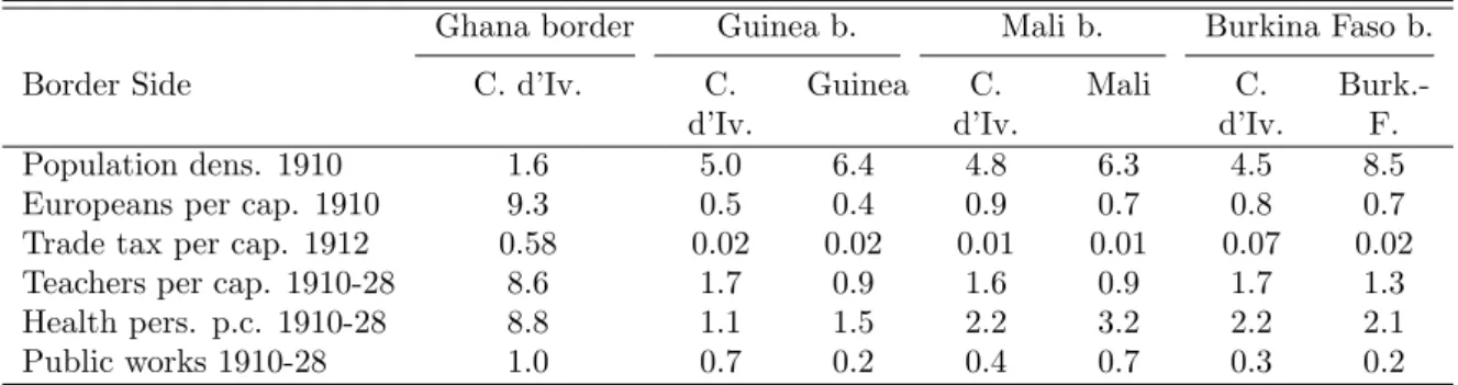
empire (Mali and Guinea). Pairwise comparisons do not reveal significant differ-ences in terms of European settlement, tax revenue, or public expenditures (see table S1.1 in the supplemental appendix). One exception is perhaps that the Mali border districts exhibited higher population density. As we shall see in the following subsection, this feature has been reversed since then.
Geography
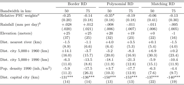
First, we check the continuity of the density of the distance to the border. The usual RD tests for sorting (Lee 2008, McCrary 2008) must be adapted to our context. We cannot only count the number of primary sample units because the sample stratification and sample rates differ between country surveys. For each bandwidth and each border size, we compute standardized “relative PSU weights” by dividing the original weights by their mean. The test then detects whether relatively more people are found closer to the border on one side compared to the other. The first row in Table 1 shows the result of this test in the case of the Ghana border. No border discontinuity is detected; one minor exception is the polynomial method at a bandwidth of 50 km. The same is found for Mali and Guinea at 75 km distance (see appendix table A.1), which will be our preferred bandwidth everywhere.
Figure 1: Map of border areas with PSUs and regional cities Atlantic Ocean Ghana Mali Burkina Faso Côte d'Ivoire Guinea Liberia Grand-Bassam Sunyani Berekum Bondoukou Abengourou Odienné Wa Man Danané Nzérékoré Grand-Bassam Sunyani Berekum Bondoukou Abengourou Odienné Wa Man Danané Nzérékoré
Note: Black dots indicate the location of primary sample units (PSUs) for the 1986–8 surveys at the Cˆote d’Ivoire-Ghana border and for the 1992–4 surveys at the borders with Mali and Guinea. Grey diamonds indicate the location of regional cities (5,000 inhabitants or more) as of 1990; city names are reported only for cities over 30,000 inhabitants. The dashed line delineates the 75 km bandwidth around the boundaries.
We then characterize the PSUs of household surveys by five geographical vari-ables: rainfall, elevation, distance to the nearest river, population density, distance to the closest regional city, and distance to the capital city (for more details on variable sources and construction, see supplemental appendix S2). The geograph-ical locations of cities with 5,000 inhabitants or more in the years 1960 and 1990
are drawn from the Africapolis database.6 Even natural geography should not be
too quickly considered to be predetermined before the drawing of the boundaries. Deforestation can influence rainfall, and even elevation or watercourses can, to some extent, be reshaped by human activity. Further, geographical discontinuities are measured on a sample of localities whose settlement is not random. However, we expect to find no or few discontinuities in rainfalls, altitude, and hydrography, and we regard this result as corroborating the quasi-randomness of the bound-aries’ alignment. Conversely, constructed geography, such as population density or city distribution, is far from being independent from boundaries. Nevertheless, we want to explore the extent to which discontinuities in welfare should be linked to discontinuities in urban structures. Finally, due to differences in countries’ shape and spatial organization, distance to the capital or main city does not vary smoothly at borders. Any border effect includes a change in the capital city and a shift in the distance to it.
The major part of the border of Cˆote d’Ivoire with Ghana does not follow a natural line, except the lagoon in the extreme South and the Black Volta river in the extreme North. Given our sample distribution, these two parts contribute little to our estimates, and withdrawing them changes nothing. The border with Ghana does not exhibit any discontinuity in our geographical variables, except distance to the capital city: the Ghana border is closer to Abidjan than it is to Accra by 130 to 150 km (table 1).
6This database from geographers (SEDET, CNRS and University Paris-7) is probably the
most complete to date. We are grateful to Eric Denis for making it available to us. We prefer not to use the urban/rural status of localities as recorded in surveys because (i) countries do not use the same definition for urban areas, and (ii) this precludes distinguishing peri-urban rural areas from more isolated ones.
The same is found for Mali in the 75 km bandwidth, except that here the border is farther away from Abidjan than from Bamako by approximately 300 km (top panel of table A.1). On both sides, as seen in figure 1, very few PSUs are found on the western part, which is underpopulated, probably due to the prevalence of parasitic diseases. Again, withdrawing the two or three most western PSUs (above longitude 7◦W) is innocuous. When enlarging the bandwidth to 100 km, additional Ivorian PSUs are found to lie relatively farther away from the border in the South. Their inclusion produces a significant “matching RD” discontinuity in rainfall. This leads us to prefer the narrower 75 km bandwidth.
Table 1: Geographical variables at the border of Cˆote d’Ivoire with Ghana
Border RD Polynomial RD Matching RD
Bandwidth in km: 50 75 50 75 50 75
Relative PSU weightsa -0.25 -0.14 -0.35* -0.19 -0.06 -0.13
(0.20) (0.18) (0.18) (0.18) (0.41) (0.30)
Rainfall (mm per day)b +.028 +.012 -.008 -.011 -.011 -.005
(.020) (.021) (.006) (.007) (.006) (.005)
Elevation (meters) +25 +25 +20 +19 +0 -1
(37) (25) (32) (23) (22) (16)
Dist. nearest river (km) -1.5 -1.1 +4.0 +3.5 +0.1 -1.5
(8.9) (6.6) (6.4) (5.3) (5.4) (4.0)
Dist. city 5,000+ 1960 (km) +14.1 -3.7 -3.2 -8.3 +6.9 +0.2
(16.0) (15.7) (20.0) (16.9) (30.3) (23.4)
Dist. city 5,000+ 1990 (km) -6.3 -13.5 -18.1 -21.3 -5.9 -10.4
(11.0) (8.8) (11.9) (12.8) (15.1) (11.9)
Pop. density 1990 (inh./km2) -5.9 -17.5 +3.7 -17.7 -6.3 -4.4
(11.2) (26.3) (10.3) (12.9) (7.6) (9.7)
Dist. capital city (km) -131*** -136*** -150*** -153*** -137*** -140***
(14) (14) (13) (13) (22) (19)
Source: Authors’ analysis based on data described in the text.
Coverage: PSUs in the bandwidth window (50 or 75 km from the corresponding border).
Notes: See equations (2), (3), and (4) for each estimator. For “Border RD” and “Matching RD”, the only control variable is latitude.
a: Probabilistic weights with means standardized to one on each side of the border. Non-weighted estimates. b: Average over the 1984–2001 period.
Positive numbers indicate differences in favor of Cˆote d’Ivoire. Standard errors in parentheses.
***: p < .01; **: p < .05 ; *: p < .10
In both the Ghana and Mali cases, the Cˆote d’Ivoire side is slightly more urbanized. Although not significantly so, Ivorian localities lie closer to the regional
cities of 1990 by 6 to 21 (Ghana border, table 1) or 7 to 13 km (Mali border, table A.1), depending on the estimates. However, the BDs are reversed when considering the distance to locations that were already cities in 1960, especially at the Mali border. We link this post-independence urbanization process to the rapid economic growth of Cˆote d’Ivoire and, more locally, to the expansion of either cocoa (Ghana) or cotton (Mali) production. Lower population density on the Mali side could also be linked to the persistence of ”river blindness” (onchocerciasis), which was previously fought and eradicated in Cˆote d’Ivoire.
Finally, in the case of Guinea, half of the alignment is based on rivers; “parts of watercourses, from map evidence, are tortuous, indecisive and many-armed” (Brownlie 1979, 374). The southern part of this border is also rather mountainous. A few discontinuities are found for elevation and distance to rivers that could put the BD estimates in question. We give it less weight in our comments and conclusions. However, no discontinuity in welfare will be identified at this border.
III.
Data and main results
After a short presentation of the survey data, we analyze border discontinuities in development outcome variables.
Survey data on development outcomes
We gather a database composed of 15 multi-topic household surveys: seven for Cˆote d’Ivoire, six for Ghana, one for Mali, and one for Guinea. These surveys were implemented between 1986 and 1998 (table A.2). We mainly use “income surveys”, which correspond to the frame of Living Standard Measurement Surveys (LSMS),
as designed by the World Bank in the 1980s. These surveys allow the measurement of consumption and income sources, and we code the geographical location of PSUs with precision using the locality name. We complement these income surveys with Demographic and Health Surveys (DHS), which do not measure consumption but record anthropometric data as well as housing conditions. All sample designs are two-stage and regionally stratified, and each PSU contains between 12 and 25 households.
We choose to analyze four different welfare outcomes: consumption per capita, children’s height-for-age, access to electricity, and access to a man-made source of water. Despite the multi-topical nature of these surveys, very few other welfare outcomes are usable for comparison.
First, we construct a household expenditure variable that includes all current expenditures, such as food, clothing, transportation, housing, and imputed rents, and expenditures for education. We only exclude overly infrequent or badly mea-sured expenditures such as those in health, durable goods, and transfers. Except for Mali, we also compute the value of the consumption of own food production, which we add to household expenditures to obtain a total consumption variable. We use monthly data on the national consumer price index and express individ-ual household consumption at 1988 or 1993 prices. Comparisons of household consumption levels are made in US dollars at 1988 or 1993 exchange rates and prices.7 We consider one important component of agricultural income, household
production of the three main cash crops produced in the region: cocoa, coffee and cotton. We retain the value of output sold, either as directly reported by the house-holds (Ghana and Guinea borders) or as physical quantities priced at the official
and uniform producer price (Mali border; the Malian survey only records physi-cal cotton output). We also extract data on wage incomes earned by household members.
Second, height stature is available for children from six months to four years (59 months) of age, and only for 6-35 months in some DHS. We construct height-for-age Z-scores using the World Health Organization standards (WHO 2006) and code children as stunted when the Z-score is below -2.
Third, from both types of surveys, we construct a dummy variable indicating whether the household uses electricity as the main source of light in the house. The surveys do not distinguish between being connected to a network or using a private generator.
Fourth and last, a second dummy variable codes whether the household has access to a man-made source of water (i.e., any source of water other than rivers, lakes, pools, or rainfalls) (Ghana border only).
The border with Ghana
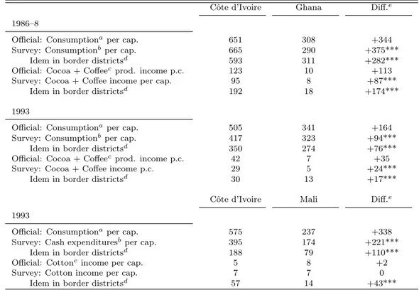
For the 1986–8 period, both national accounts and income surveys provide similar figures for consumption per capita in the two countries. Cˆote d’Ivoire appears wealthier than Ghana by a large 344-375 USD gap at 1988 prices and exchange rates (table 2, upper top panel). Cocoa and coffee income figures computed from FAO data and from surveys are also quite consistent. When restricting the com-parison of survey means to the sub-sample of administrative districts lying along the boundary, the gap in consumption is slightly reduced but remains as large as 282 USD, whereas the cash crop income difference widens to +174 USD because
the Ivorian side is a very important cocoa and coffee production area. The year 1993 marked the climax of an enormous macroeconomic crisis in Cˆote d’Ivoire, triggered by the collapse of international prices for cocoa and coffee in 1987 and the halving of administered producer prices in 1990. In contrast, Ghana began a progressive recovery from two decades of economic and political turmoil. In the case of Cˆote d’Ivoire, survey figures exhibit a greater fall than national accounts (table 2, lower top panel). This may be due to under-reporting biases in the less detailed 1992–3 survey and/or to the inaccuracy of national accounts, which compute private consumption as a residual. Cˆote d’Ivoire remains the wealthiest country, even in border districts, where a significant gap of +76 USD per capita is observed. Cash crops’ income differences remain statistically significant but are ten-fold lower (+17 USD). Unfortunately, the absence of geographical coordinates in the 1992 Ghanaian income survey prevents us from using these consumption and income figures for the computation of BDs.
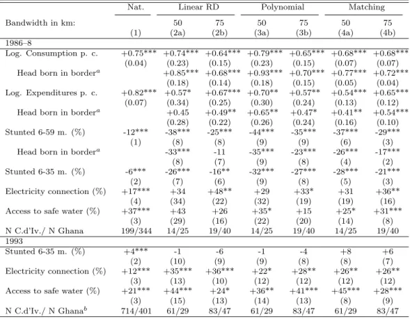
The BD estimates are reported in table 3, again for the two periods of 1986–8 (top panel) and 1993 (bottom panel), and for the set of four welfare indicators. Column (1) reports the difference between survey means at the national level, and columns (2a) to (4b), respectively, report the BD obtained when implementing our three estimation methods with two bandwidths, 50 or 75 km, as in table 1. In 1986–8, we are able to restrict the estimates to the sub-sample of heads born in border administrative districts and in the country of residence. This allows us to test whether discontinuities hold among people sharing the same region of origin or “ethnicity” because part of the above-mentioned literature is concerned with this dimension, especially the fact that shared preferences or intense trade flows may equalize welfare among ethnic groups. We favor the district of birth variable
Table 2: National accounts and Survey means: Cˆote d’Ivoire, Ghana and Mali
Cˆote d’Ivoire Ghana Diff.e
1986–8
Official: Consumptionaper cap. 651 308 +344
Survey: Consumptionbper cap. 665 290 +375***
Idem in border districtsd 593 311 +282***
Official: Cocoa + Coffeecprod. income p.c. 123 10 +113
Survey: Cocoa + Coffee income per cap. 95 8 +87***
Idem in border districtsd 192 18 +174***
1993
Official: Consumptionaper cap. 505 341 +164
Survey: Consumptionbper cap. 417 323 +94***
Idem in border districtsd 350 274 +76***
Official: Cocoa + Coffeecprod. income p.c. 42 7 +35
Survey: Cocoa + Coffee income p.c. 29 5 +24***
Idem in border districtsd 30 13 +17***
Cˆote d’Ivoire Mali Diff.e
1993
Official: Consumptionaper cap. 575 237 +338
Survey: Cash expendituresbper cap. 395 174 +221***
Idem in border districtsd 188 79 +110***
Official: Cottoncincome per cap. 5 8 +2
Survey: Cotton income per cap. 7 7 0
Idem in border districtsd 57 14 +43***
Source: Authors’ analysis based on data described in the text.
Notes: Figures in US dollars. Top panel (Ghana): 1988 prices and exchange rates. Bottom panel (Mali): 1993 prices and exch. rates. 1986–8: Averages of 1986–8.
a: National accounts household final consumption expenditure per capita.Source: World Bank 2012.
b: Top panel (Ghana): Household consumption per capita, including consumed own food production. Bottom panel (Mali): Household cash expenditures per capita.
c: Cocoa beans, green coffee, or seed cotton output multiplied by the corresponding producer price and divided by total population. Source: FAOSTAT 2012.
d: Administrative districts lying along the border. Ghana border: Abengourou, Aboisso, Agnibil´ekrou,
Bondoukou, Tanda (Cˆote d’Ivoire side); Western and Brong-Ahafo (Ghana side). Mali border: Boundiali,
Ferkess´edougou, Korhogo, Odienn´e, and Tingr´ela; Bougouni, Kadiolo, Kolondi´eba and Yanfolila. See also map
S2.1 in the supplemental online appendix.
e: Difference between the first and second columns. For survey means comparisons, errors are clustered by PSUs: ***: p < .01; **: p < .05 ; *: p < .10
over the Akan ethnic group variable because the GLSS1 survey for 1987 Ghana has many (non-random) missing values for ethnicity.
Table 3: Discontinuities at the border of Cˆote d’Ivoire with Ghana
Nat. Linear RD Polynomial Matching
Bandwidth in km: 50 75 50 75 50 75
(1) (2a) (2b) (3a) (3b) (4a) (4b)
1986–8
Log. Consumption p. c. +0.75*** +0.74*** +0.64*** +0.79*** +0.65*** +0.68*** +0.68***
(0.04) (0.23) (0.15) (0.23) (0.15) (0.07) (0.07)
Head born in bordera +0.85*** +0.68*** +0.93*** +0.70*** +0.77*** +0.72***
(0.18) (0.14) (0.18) (0.15) (0.05) (0.04)
Log. Expenditures p. c. +0.82*** +0.57* +0.67*** +0.70** +0.57** +0.54*** +0.65***
(0.07) (0.34) (0.25) (0.30) (0.24) (0.13) (0.12)
Head born in bordera +0.45 +0.49** +0.65** +0.47* +0.41** +0.54***
(0.28) (0.22) (0.26) (0.24) (0.16) (0.10)
Stunted 6-59 m. (%) -12*** -38*** -25*** -44*** -35*** -37*** -29***
(1) (8) (8) (9) (9) (6) (3)
Head born in bordera -33*** -11 -35*** -23*** -26*** -17***
(8) (7) (9) (8) (4) (2)
Stunted 6-35 m. (%) -6*** -26*** -16** -32*** -27*** -28*** -21***
(2) (7) (6) (9) (8) (5) (3)
Electricity connection (%) +17*** +34 +48** +29 +33* +31 +36**
(4) (34) (22) (32) (19) (19) (16)
Access to safe water (%) +37*** +43 +26 +35* +15 +25* +31***
(3) (29) (16) (22) (20) (14) (8) N C.d’Iv./ N Ghana 199/344 14/25 19/40 14/25 19/40 14/25 19/40 1993 Stunted 6-35 m. (%) +4*** -1 -6 -1 -4 +8 +6 (2) (10) (9) (9) (8) (8) (7) Electricity connection (%) +12*** +35*** +36*** +22* +28** +26** +26** (3) (13) (10) (12) (12) (12) (12)
Access to safe water (%) +21*** +44*** +24* +36** +41*** +45*** +28***
(3) (15) (13) (14) (13) (8) (9)
N C.d’Iv./ N Ghanab 714/401 61/29 83/47 61/29 83/47 61/29 83/47
Source: Authors’ analysis based on data described in the text.
Coverage: PSUs in the bandwidth window (50 or 75 km from the corresponding border).
Notes: Consumption and expenditures at 1988 prices and exchange rates. Col. (2a) to (4b): controls for latitude, rainfalls, elevation, and distance to river are always included.
a: Head born in border: Household head is born in a district lying along the border (see table 2 footnote d).
b: Income survey pooled with DHS data on the Cˆote d’Ivoire side, DHS only on the Ghana side.
Positive numbers indicate differences in favor of Cˆote d’Ivoire. Standard errors in parentheses.
***: p < .01; **: p < .05 ; *: p < .10
In 1986–8, significant BDs are found for log consumption per capita, ranging from +0.64 to +0.93 (i.e., indicating large income gaps at the border of the two countries) even if we restrict to households whose head is a native of border
dis-tricts. BDs for log cash expenditures support the same conclusions, although they are lower on average (+0.41 to +0.70).
Although we discuss the channels driving these results in more detail in section IV, we need to assess the role of differences in price levels because discontinuities in “nominal” consumption may not match discontinuities in purchasing power. According to the World Bank (2012), in 1988, the price level of private consumption in Cˆote d’Ivoire was 0.98 that of Ghana, whereas according to the Penn World Tables 7.1 (Heston, Summers and Aten 2012), it was 1.09 at official 1988 exchange rates (i.e., 298 CFA francs and 202 cedis for one US dollar, respectively). After 1983, the Ghanaian government began a gradual process of devaluation of the cedi that ended with free float in 1990 and the elimination of the black market premium. In 1988, the parallel market exchange rate was estimated at 252 cedis/USD.8Using this parallel exchange rate instead of the official one would enhance the border discontinuities in consumption by a factor of 1.25 (=252/202). Thus, it is hardly plausible that the real exchange rate holding in border areas could reverse the conclusion of a large discontinuity in real consumption per capita.9
Furthermore, the figures for the share of stunted children are consistent with the Cˆote d’Ivoire advantage in consumption. For children six months to four years of age, we find large and robust BDs, ranging between 19 and 44 percentage points, with only one exception (linear RD with 75 km bw and heads born in border districts). For the sub-sample of younger children (6 to 35 months), the point
8Data from Robert Bates, Karen Feree, James Habyarimana, Macartan Humphreys, and
Smita Singh. 2001. “Economic Data (updated 2005)”, http://hdl.handle.net/1902.1/14978 UNF:5:8vHsoDT1Q8sUbiTZgDkctw== Murray Research Archive [Distributor] V1 [Version].
9In a completely different context, Gopinath, Gourinchas, Hsieh, and Li (2011) find retail and
wholesale markets to be segmented at the border between Canada and US. However, relative prices co-move with the nominal exchange rate, so there is little room for changes in the real exchange rate.
estimates lie between 16 and 32 pp. In 1993, which is when income differences at the border must have been reduced to a minimum (see table 2 and above), BDs in early-age stunting are no longer observed. For Cˆote d’Ivoire, Cogneau and Jedwab (2012) found that the 1990 drastic cut in cocoa producer prices had a large impact on the height of two- to five-year-olds, less so on the youngest.
Finally, BDs for access to electricity seem large in magnitude for most esti-mates; they are always above 29 percentage points in 1986–8 but suffer from a lack of precision when the smallest 50 km bandwidth is used. BDs for access to safe water are positive but even less precise. With larger sample sizes on the Cˆote d’Ivoire side in 1992–3, both are found to lie in the same range and display higher statistical significance.10 The results are not shown for the year 1998; despite a small sample on the Ivorian side (11 PSUs only), the results seem to confirm the persistence of the relative superiority of Cˆote d’Ivoire over Ghana in terms of utilities.11
The northern borders
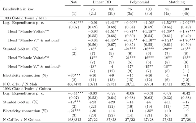
We now turn to the northern borders of Cˆote d’Ivoire with Mali and, secondarily, Guinea.12
Although 1993 was a very bad year for Cˆote d’Ivoire, the macroeconomic fig-ures in table 2 show that this country was still far above Mali in terms of household
10Using DHS data only and for the 75 km bw, the results are similar, although again less
precise due to the smaller sample size (for electricity connection: +44**, +40*, +35; for water safety: +27*, +44***, +32**).
11For the 75 km bw and for 1998, the results for electricity connection are +81***, +63***,
+48**; for water safety: +30*, +20, +19**.
12In previous versions of this work, we also looked at the border with Burkina Faso. However
identification had drawbacks due to sample size and distribution. Borders between northern neighbors were also studied. See supplemental appendix section S3.
consumption per capita, by around +300 USD at 1993 exchange rates and prices. This national account figure is consistent with the survey means comparison for cash expenditures (+221 USD difference), although with some caveats already mentioned. When focusing on administrative districts along the border, the ad-vantage of the Cˆote d’Ivoire side is halved but remains significant at approximately +110 USD. Even if cotton output per capita was fairly comparable at the national level, the Malian border districts produced very little cotton in 1993, providing a +43 USD per capita advantage to Ivorian districts.
Particularly because of its bauxite resources, Guinea is wealthier than Mali, and the difference from Cˆote d’Ivoire only reaches +200 USD in consumption per capita (not shown). Furthermore, although mines are not located in the border areas, survey mean comparisons among border districts show that the Guinean side is no poorer than the Ivorian side (not shown).
At the Mali border, discontinuities in log cash expenditures per capita are even higher than those found at the border with Ghana, ranging from +0.84 to +2.02 depending on the estimates, the bandwidth used, and the population considered (table 4 top panel). Recall, however, that the narrower 75 km bandwidth can be deemed more reliable for identification (see above). With this bandwidth, the upper bound is decreased to +1.52. The restriction to household heads who are from the Mande-Voltaic group again slightly reduces the estimates by dropping a few Ivorian southerners, such as civil servants sent to the North.13 When we
ad-13The Mande include, in particular, the Bambara, Bobo, Diula, Malinke, and Soussou, whereas
the Voltaic or Gur include the Lobi, Mossi, and Senoufo people. The Mande and Voltaic groups are close together in linguistic terms and display some mixing on the map. Ethnic codifications are not homogeneous; in particular, the Malian survey records the language of interview rather than the “ethnic group”. However, district of birth is only recorded in the Cˆote d’Ivoire survey, so we have no alternative.
ditionally withdraw international migrants (i.e., mainly relatively wealthy Malian migrants to Ivorian regional cities such as Korhogo), a slight attenuation is again observed, but the BDs still range between +0.8 and +1.2.
Table 4: Discontinuities at the border of Cˆote d’Ivoire with Mali and Guinea
Nat. Linear RD Polynomial Matching
Bandwidth in km: 75 100 75 100 75 100
(1) (2a) (2b) (3a) (3b) (4a) (4b)
1993 Cˆote d’Ivoire / Mali
Log. Expenditures p. c. +0.89*** +0.91 +1.41** +0.90** +1.06* +1.52*** +2.02***
(0.07) (0.59) (0.68) (0.34) (0.59) (0.64) (0.49)
Head ”Mande-Voltaic”a +0.93 +1.51** +0.87** +1.18** +1.39** +1.88***
(0.55) (0.66) (0.30) (0.54) (0.61) (0.49)
Head ”Mande-V.” & nationala +0.84 +1.45** +0.76** +1.10** +1.21* +1.70***
(0.56) (0.67) (0.35) (0.55) (0.61) (0.50)
Stunted 6-59 m. (%) +2 -13* -3 -21*** -16*** -20** -16**
(2) (7) (9) (6) (6) (7) (8)
Head ”Mande-Voltaic”a -14** -7 -21*** -16*** -18** -16**
(7) (9) (5) (5) (8) (8)
Head ”Mande-V.” & nationala -13* -4 -17* -15** -18** -16
(7) (12) (9) (7) (8) (11)
Electricity connection (%) +36*** +10 +9 +15 +16 -1 +1
(2) (11) (13) (15) (12) (6) (12)
N C. d’Iv. / N Mali 468/473 13/11 32/31 13/11 32/31 13/11 32/31
1993 Cˆote d’Ivoire / Guinea
Log. Expenditures p. c. +0.44*** -0.03 -0.28 -0.08 +0.31 -0.07 -0.42 (0.07) (0.53) (0.64) (0.68) (0.62) (0.32) (0.38) Stunted 6-59 m. (%) +12*** +23 +29 +14 +5 +11 +17 (2) (22) (22) (16) (19) (11) (17) Electricity connection (%) +21*** +30 +14 +11 +35* +10 +9 (3) (20) (22) (14) (21) (6) (8) N C.d’Iv. / N Guinea 468/312 27/22 37/28 27/22 37/28 27/22 37/28
Source: Authors’ analysis based on data described in the text.
Coverage: PSUs in the bandwidth window (50 or 75 km from the corresponding border).
Notes: In the cases of “Border RD” and “Matching RD” and for 100 km bandwidth (col. 2b & 4b), sample sizes allow for using a quadratic in distance to border rather than a simple linear specification. Col. (2a) to (4b): controls for longitude (Mali) or latitude (Guinea), rainfalls, elevation, and distance to river are always included. a: Head from a Mande or a Voltaic linguistic group. National: excluding foreign immigrants.
Positive numbers indicate differences in favor of Cˆote d’Ivoire. Standard errors in parentheses.
***: p < .01; **: p < .05 ; *: p < .10
Here, monetary welfare comparisons are facilitated by the fact that the two countries share the same currency, namely the CFA franc. We acknowledge that the BDs in nominal consumption may mix discontinuities in real terms and in
price levels. However, although cattle is a traditional export of northern countries and kola nut is a traditional export of forested Cˆote d’Ivoire, many goods flow one way or another across the border depending on market demand (e.g., cereals such as rice or millet, textiles, spare parts, etc.), so persistent price differentials should be limited (Labaz´ee 1993). At the national level, World Bank (2012) figures for the year 1993 indicate that the price level of private consumption was lower in Mali by a factor of 0.81; Heston, Summers, and Aten (2012) report a ratio of 0.75. Even if they prevailed at the border, these orders of magnitude would not cancel out the large BDs in real consumption. The devaluation of the CFA franc in 1994 creates an additional difficulty in the comparison because the Malian income survey was implemented in the middle of this year (between March and June), whereas the Ivorian survey was conducted over 1992 and 1993. As already mentioned, monthly prices were used to correct for inflation. The average deflator for cash expenditures in Mali (i.e., the ratio of 1993 prices to current prices) is 0.90, indicating a 10% inflation rate six months after the 50% devaluation. Again, we checked that the Cˆote d’Ivoire advantage was preserved even when we do not deflate the consumption and income variables for Mali.
Furthermore, the BDs for the share of stunted children are again consistent with consumption figures, whereas no difference in national averages is observed. In addition to income, climate and ecology strongly determine height in Africa (Moradi 2012). In West Africa, all anthropometric data confirm that people from the savannah are taller than people from the forest because of the protein intake they obtain from milk and meat (cattle breeding is constrained in the South by the presence of the tsetse fly). In the Malian survey, children from the North were taller than children born close to the Cˆote d’Ivoire border. Thus, when restricting
the comparison to the same ecological area, we recover large BDs in nutrition: within our preferred 75 km bandwidth, children from the Cˆote d’Ivoire side are 13 to 21 pp less likely to be stunted. The next section will provide some evidence that the bulk of this discontinuity can be explained by parental income.
Finally, whereas the average Ivorian household is 36 pp more likely to have electricity compared to its Malian counterparts (col.1), we find no evidence of a discontinuity in electrification at the border.
In the case of the border with Guinea, no BDs in consumption per capita, stunting, or access to electricity are found (bottom panel of table 4).
IV.
The role of public policies
We argue that two main factors determine the presence or absence of discontinuities in welfare at the borders of Cˆote d’Ivoire with its neighbors. The first factor lies in the public policies that regulate the cash crop sectors (here, cocoa, coffee, and cotton), either through administered producer prices or through agricultural extension and subsidies to production. The second factor is public investment, either national or local, in infrastructures and utilities such as electricity and safe water.
Because cash crop income is mainly derived from rural areas, whereas utilities initially reach cities, we introduce the urban structure into the analysis. This approach also allows us to test the robustness of our BD estimates. We use a variable already considered in the subsection dedicated to geography, the distance to cities with more than 5,000 inhabitants in 1990. Due to sample size constraints, we only distinguish two urbanization classes: 0 to 5 km from a city and 5 km or
more. We then compute new “matching RD” estimates with PSUs matched with the nearest neighbor from the same class.14 We report matching RD estimates
for the whole sample (”All”) and for the sample restricted to remote rural areas (”5+”); we do this for our preferred 75 km bandwidth. The results show that the “All” and “5+” estimates look very much the same. Indeed, cities or peri-urban areas (”0-5”) are seldom found close to the borders, and it is mainly differences between remote rural areas that ”make” the border discontinuities (table 5). In addition to this “urban/rural” breakdown, we report BD estimates for cash crop output and income.
At the border with Ghana (1986–8), BDs in log cash expenditures are very robust to the breakdown between urban/peri-urban (0-5 km) and remote rural (5+ km) localities. For the whole sample (col.1a), the matching RD estimate of +0.62 compares with the initial finding of +0.65 in table 3 col.(4b). When restricting to rural areas (col.1b), it decreases to +0.52 but remains highly significant. At the border with Mali (1993), where a large majority of PSUs is rural, the same restriction leads ato a significant BD of +0.86 in log cash expenditures (col.2b). At the border of Guinea (1993–4), it is still the case that no discontinuity is detected (col.3).
We now turn to cash crop output and income.
At the Ghana border, no discontinuity in cocoa output is detected; both sides are important cocoa production areas at that time.15 However, the real producer
price for cocoa in Cˆote d’Ivoire is more than twice that of Ghana: at 1988 prices,
14For the rest, the estimation is kept the same; see equation (4). In the case of the Mali border,
where only five urban or peri-urban PSUs are found in the 75 bandwidth, we match these five PSUs with the nearest neighbor, regardless of its urbanization class. See also table 5 footnote.
15At the national level, the Ivorian superiority in cocoa output is due to the younger trees of
Table 5: The cash crops channel
Ghana Mali Guinea
1986–8 1993 1993
Distance to city in km: All 5 + All 5 + All
Bandwidth in km: 75 75 75 75 75
(1a) (1b) (2a) (2b) (3)
Log. Expenditures per capita +0.62*** +0.52*** +1.52*** +0.86** -0.22
(0.13) (0.13) (0.64) (0.31) (0.22)
Main cash cropcoutput p.c. (kg) +29 +23 +733*** +664*** +9**
(30) (46) (211) (84) (3)
Cash cropsbincome p.c. (USD)a +194*** +184*** +237*** +214*** +16***
(43) (65) (68) (27) (2)
Cash Expenditures per capita (USD)a +177*** +120** +173** +117*** +2
(52) (48) (61) (38) (37)
Cash crops inc. controlledd +135 -2 +48 -13 +63
(99) (77) (56) (32) (64)
Cash crops & wage inc. controllede +21 -1 +39 -13 -31
(53) (65) (53) (39) (20)
Stunted 6-59 months (%) -26*** -32*** -20** -24*** +16
(6) (5) (7) (7) (13)
Expend. per cap. controlledf -10 -8 -5 -8 +14
(7) (5) (12) (14) (13)
Electricity connectiong (%) +28** +22* -2 -6 +0
(13) (11) (6) (4) (4)
N 19/40 10/30 13/11 10/9 27/22
Source: Authors’ analysis based on data described in the text. Coverage: PSUs in the 75 km bandwidth window.
Notes: “Matching RD” estimates with 75 km bandwidth. PSUs are matched to the nearest neighbor on the other side of the border within the same urbanization class: 0-5 km or 5+ km from the nearest city (5,000 + inhabitants) as of 1990. Matched differences are then analyzed as in equation (4) (see text). In the case of the Mali border, where only 5 PSUs are in the 0-5 km class, the “All” estimate (col.2a) does not match PSUs according to class, it is therefore exactly the same as in Table 4 col. (4a). Controls for latitude (Ghana and Guinea) or longitude (Mali), rainfalls, elevation, and distance to river are always included.
a: 1988 prices and exchange rates in columns (1a-b); 1993 prices and exchange rates in col. (2a-b) and (3). b: Cocoa and coffee sales in (1a-b) and (3); Cotton output valued at official producer price in (2a-b). c: Cocoa output sold in col. (1a-b) and (3); Cotton output in col. (2a-b). Kilograms per capita.
d: Cash expenditures per capita border discontinuity, with cash crop income per capita added as a control. e: Idem d, with instead the sum of cash crop and wage income per capita as a control.
f: Stunted children discontinuity, with cash expenditures per capita and its square added as controls.
g: At the border with Ghana in 1992–3 and for electricity connection: ’All’: +30** (s.e. 13); ’5+’: +37** (16).
Positive numbers indicate differences in favor of Cˆote d’Ivoire. Standard errors in parentheses.
the average real producer price for 1986–8 is 1.55 USD per kg in the former country compared with 0.65 in the latter. In contrast, in the case of coffee, a large BD in output is observed because this crop is not produced in Ghana due to historically low administered producer prices in this country. Among rural villages, we there-fore find a large BD in cocoa and coffee income of +184 USD per capita (table 5, col. 1b). Additional disaggregation (not shown) shows that cocoa accounts for two-thirds and coffee for the remaining one-third. Before 1990, the cocoa producer price differential generated a strong incentive to smuggle cocoa beans across the Cˆote d’Ivoire border (Bul´ır 1998). However, our BD result suggests that smuggling was not widespread enough to equalize incomes across the border. When the cash crop income variable is added as a control in the BD estimates, the BD in cash ex-penditures that prevails among rural villages is strikingly erased, decreasing from +120 USD to a negligible -2 USD. Recall that expenditures and income figures are drawn from two independent parts of the surveys’ questionnaires.16 When
including cities and peri-urban villages (col. 1a), the cash expenditure disconti-nuity is only reduced from +177 to +135 USD, although it becomes statistically insignificant. However, if we add formal wage income earned by household mem-bers to cash crop income, then controlling for this new income variable successfully reduces the cash expenditures BD to a low and insignificant +21 USD.17
At the Mali border, we detect a very large BD in cotton output per capita of +664 kg per capita among rural villages (col.2b). In contrast with the Ghana
16This procedure involves assuming that (i) the same saving rate applies to cash crop income
on both border sides and (ii) this saving rate is consistently estimated by OLS.
17In 1986–8, the survey figures for the average annual wage of civil servants and public firms
workers reached 5,223 USD in Cˆote d’Ivoire compared with 663 USD in Ghana. For private firm workers, they were 3,498 USD and 540 USD, respectively. The minimum wage in Cˆote d’Ivoire (1,400 USD) was also six times higher than in Ghana (240 USD).
border, the BD in cotton income mainly stems from a higher output on the Cˆote d’Ivoire side because producer prices are only slightly higher (90 vs. 85 CFA franc per kg in Mali). Further, this Ivorian advantage is specific to the border area; both national official sales and survey figures show that the two countries produced roughly the same quantities of cotton (see table 2). In fact, the Mali side of the border was not yet producing significant quantities of cotton. In this country, cotton production historically began more northward, around the city of Koutiala, and mostly took off in the mid-1970s. As in Cˆote d’Ivoire, it was strongly regulated and subsidized by the State through a parastatal company (Compagnie Malienne
de D´eveloppement des Textiles). We can again explain the BD in consumption
among rural villages by the discontinuity in cash crop income. As in the case of Ghana (with cocoa and coffee), when controlling for cotton income, the BD in cash expenditures decreases from +117 USD to an insignificant -13. Unreported results also show that richer farmers invest in cattle. We identify BDs in the number of cows owned by the household (+1.76, s.e.= 0.32) as well as in the number of goats and sheep (+0.53, s.e.=0.10). Differences in public health policies may also be involved because the fight against parasitic diseases (river blindness or onchocerciasis, sleeping sickness or trypanosomiasis) was undertaken much earlier in Cˆote d’Ivoire.
At the Guinea border, although almost no cocoa and approximately half as much coffee is grown on the Guinea side, the BD in cash crops income is small but statistically significant (+16 USD). In comparison with the Ghana and Mali cases, we argue that the absence of a large difference in cash crop income may account for why no border discontinuity is found in consumption per capita or in children’s stunting.
Regarding this latter variable, table 5 also suggests that a large part of the BDs can be accounted for by household consumption. In the Ghana case, controlling for cash expenditures per capita and its square reduces the BD in stunting from -32 among rural villages (-26 in the whole sample) to an insignificant -8 percent (-10 in the whole sample). In the Mali case, the same dramatic reduction is observed, from -24 in rural villages to -8 percent (-20 to -5 in the whole sample). Combined with the results obtained on the impact of cash crop income, this last result lends some support to the idea that the cash crop channel explains most of the border discontinuities in both household consumption and child nutrition.
In the Ghana case, electricity reaches border rural villages on the Cˆote d’Ivoire side, whereas none of their Ghanaian counterparts is connected. This simple fact translates into a significant +22-percentage-point BD (+28 pp in the whole sample, see last row of table 5). In 1993, these BDs were reinforced: +37 pp in rural areas and +30 in the whole sample (see table 5 footnote). The same features are found for access to safe water. In contrast, at the two other borders, all remote rural areas are in the dark. Although Ivorian regional cities are more connected to electricity than their northern counterparts, they are too far from the border to significantly contribute to the BDs. In explaining these features, it is difficult to disentangle a pure wealth effect from a more discretionary uneven allocation of public investment.18
Recent history shows that price policies were reverted during structural ad-justment under pressure from donors. In 1989–90, Cˆote d’Ivoire halved both its cocoa and coffee producer prices before raising them again after the CFA franc
18Although wealthier, northern Ivorian households may not be wealthy enough to pay for
devaluation in 1994. In the meantime, Ghana significantly raised its cocoa pro-ducer price so that the difference between the two countries became negligible at the end of the 1990s. Changes in cash crop production were slower, but they also occurred. Between 1994 and 2001, Mali more than doubled its cotton production in the South through the extensive cultivation of new lands; however, the cultiva-tion of cotton had not yet reached the most southern border area (Dufumier and Bainville 2006). In contrast, the Ivorian “cocoa frontier” has moved westward and today reaches the southern Guinea border. With these developments, some of the border discontinuities that we identified for the 1990s may have changed. After 2002, the civil war in Cˆote d’Ivoire and the five-year partition between North and South may have further reduced the Ivorian advantage at the northern borders, at least until 2007. In the South, Ghana continued to catch up with its neighbor (Eberhardt and Teal 2010). Hence, although infrastructure showed greater per-sistence in 1993 and in 1998, border differences may have been attenuated since then. Unfortunately, the data that we gathered do not cover those more recent economic conditions.
V.
Conclusion
The borders between Cˆote d’Ivoire and its neighbors divide fairly comparable ar-eas in terms of geography, anthropology, and precolonial history. At the end of the 1980s and in the 1990s, Cˆote d’Ivoire was by far the wealthiest country, par-ticularly because of its export crops. By applying regression discontinuity designs to a set of household surveys, we show that this higher wealth was translated at the borders with Ghana and Mali in the form of large and consistent