Background Paper
Household risk
management in Senegal
Philippe De Vreyer
University of Paris Dauphine
Sylvie Lambert
Household risk management in Senegal.
Philippe De Vreyer (PSL, University of Paris Dauphine, LEDa, UMR DIAL and IRD) Sylvie Lambert (Paris School of Economics‐INRA) June 2013 It is an accepted fact in the economic literature that households in developing countries have to find informal ways either to limit exposure to risk or to cope with shocks ex‐post, since they face a risky environment that lacks formal insurance institutions. A large number of papers, starting with Rosenzweig (1988) and reviewed for example in Dercon (2002), discuss the form and efficacy of households’ strategies with regards to risk management and risk coping. Less often discussed is the issue of intra‐household allocation of shock consequences, apart for the gender difference. In fact, some papers (e.g. Rose 1999) try to assess whether shocks suffered by a household have similar impacts on boys and girls. In the Indian context, it is found that boys are better sheltered from the adverse impacts of weather shocks. Dercon and Krishnan (2000) examine the differential impact of shocks on health outcome for male and female family members in Ethiopia and show that women endure more negative short term impacts.In the West African context where extended family is the common form of living arrangements, inequality may exist along other lines than the gender divide. Which household members happen to be in the most vulnerable positions in case of shock is of major public policy relevance but has never been studied so far, probably due to the lack of adequate data. This question motivates the present paper.
This paper explores risk management and risk coping by Senegalese households, with a focus on individual vulnerability to shocks within the household. This is made possible thanks to unusually detailed data on intra‐household allocation of resources: consumption expenditures are collected at the level of subgroups within the household (called cells thereafter), corresponding to distinct consumption units, as explained below.
We first document the risks faced by households in Senegal by looking at the frequency and types of shocks that households are exposed to, as well as the ways in which households cope with these shocks (both positive and negative). We then assess the impact of the shocks on household per capita consumption and on human capital accumulation, trying to identify which of the household characteristics facilitate coping. The study finally addresses the issue of the way shocks affect the intra‐household allocation of resources.
The paper is divided a follows: we first describe the household survey data that we use for this study (section 1). Then we provide descriptive statistics on the self declared shocks reported by households over a five‐year time span (section 2). Section 3 looks at the impacts of shocks on household yearly consumption and identifies the household characteristics that help mitigating or on the contrary intensify this impact. In section 4, we explore the correlates of intra‐household inequalities and whether shocks tend to exacerbate these inequalities. Section 5 assesses the impact of shocks on children schooling and hence hints at the long term impact of short term income shocks. Section 6 concludes.
1. The Data
In order to complete this task, the paper exploits data from an original survey on Poverty and Family Structure (« Pauvreté et Structure Familiale » in French, hence referred to as PSF) that we conducted in Senegal in 2006/2007 in close collaboration with the Senegalese statistical agency (ANSD) and with Abla Safir who is now with the World Bank.1 The data is described in details in De Vreyer et al. (2008).The survey was conducted over 1800 households spread over 150 clusters drawn randomly from the census districts so as to insure a nationally geographically representative sample. Only 1771 records can be exploited for the purpose of this paper.
In addition to the usual information on individual characteristics (including educational outcomes), a detailed description of household structure and budgetary arrangements is obtained from long interviews. In Senegalese households, consumption can be divided into two components to which different budgets are dedicated. First, some expenditure under the responsibility of the household head corresponds to public goods and food, which are mainly common expenditures. The rest comprises private goods accruing to relatively autonomous consumption units. This latter part is financed both by the group own specific economic resources and potentially also by contributions of other household members. This renders possible vast intra‐household consumption inequalities that might not be fully bridged by intra‐household transfers. Hence, it makes sense to collect information on the household structure in order to be able to observe consumption at the level of each of these groups. Field interviews showed that the relevant decomposition of the households into consumption units is one that associates individuals with their primary caretaker in the household. Cells are therefore defined according to the following rule: the head of household and unaccompanied dependent members, such as his widowed parent or his children whose mother does not live in the same household, are grouped together. Then, each wife and her children make a
1
Momar B. Sylla and Mata Gueye of the Agence Nationale de la Statistique et de la Demographie of Senegal (ANSD), on the one hand, and Philippe De Vreyer (University of Paris‐Dauphine and IRD‐DIAL), Sylvie Lambert (PSE) and Abla Safir (World Bank), on the other hand, designed the survey. The data was collected by the ANSD thanks to the funding of IDRC (International Development Research Center), INRA Paris and CEPREMAP.
separate group. Finally, any other family nucleus such as a married child of any member with his/her spouse and children also form separate groups. Consumption expenditures are measured at the cell level. Recall period varies by good and was left to the choice of the respondent. The data used here is an annualized measure covering the past 12 months. The survey also includes a fairly detailed section on shocks at the household level, which will prove particularly useful for our purpose. This section collects information on shocks, positive and negative, that occurred during the past 5 years (hence from 2001/2002 to 2006/2007). The nature of the shock as well as its consequences on the household are listed. The section also includes subjective assessment of the household and community standard of living, as well as their perception of isolation or inclusion in a network that can provide help in case of need or that can require support.
2. Description of shocks prevalence
a. General remark Shocks are measured from the answer to the following question: “During the past five years, did you experience a particularly good year (resp. bad year)?”. It is difficult to assess a priori the real informational content in the answer to this question. In particular, one can imagine that, as has been observed for self reported health data, what is perceived as a shock might differ along certain household characteristics, which might blur the picture in our analysis. The only way we have to try to gain some confidence in the usefulness of this information is to compare the answers to this question to those given to another set of questions dedicated to unusual expenditures. Among those, the only ones that can be related to a shock are expenses incurred in case of illness (other are ceremonial expenses or major investments). We find a positive correlation between declaring important expenses due to illness and declaring a negative shock. Further, the average amount of health expenses is 4 times higher when a negative shock is declared than when it is not the case. This underlines that indeed households indicate as shock only unusual deviations. Although this doesn’t exhaust the question, this observation is fairly reinsuring as to the informational content of the question on self reported shocks.
b. Good years
Out of the sampled households, a good third (604 households that is 34%) declares having had at least one particularly good year during the past 5 years. Clearly, recollection difficulties are an issue, since most of the good years happened from 2004 onwards and hardly any are declared for 2001/2002. In order to reduce as much as possible the potential biases due to
these difficulties, in the analysis of impact of shocks we will mostly use events occurring in the 2 years preceding the survey: 17% (305) declare a good year in 2005, 2006 or 2007.
Each household could declare up to 3 good years. Most declare only one good year (60% of those with shocks). These shocks are fairly spread out in the country since in more than 2/3 of the 150 clusters at least one household reports a positive shock.
Five types of positive shocks are registered in the survey. Table 1 shows the frequency of occurrence of each of them. The most frequently mentioned is that of a particularly good harvest, followed closely by good sales. Together, they account for 79% of the shocks for those who benefited from a favourable event. These two events are positively correlated but, in a given year, the coefficient of correlation between the two is only between 0.33 and 0.38. Hence they seem to capture different events.
The proportion of households having benefited from each of these types of shocks in the 2 years preceding the survey is given in the last column of table 1. Here again the larger prevalence of good harvest and good sales as causes for particularly good years appears clearly. In 2005, 11.7% of the households declare at least one positive shock, only 8.5% in 2006. Table 1: Type of shocks experienced by surveyed households Type of shocks Number of households % of households with positive shocks over the 5 years preceding the survey % among those with positive shocks (N=602) % of households with positive shocks in 2005/2006. Good harvest 262 14.79 43.02 7.34 Good sales 219 12.37 36.05 6.04 Inheritance 3 1.69 4.98 0.70 New employment 129 7.28 21.43 2.94 High prices 38 2.15 6.15 0.79 Other 134 7.57 22.26 3.30 Note : Multiple answers are possible ‐ Source: PSF survey data, our own calculations.
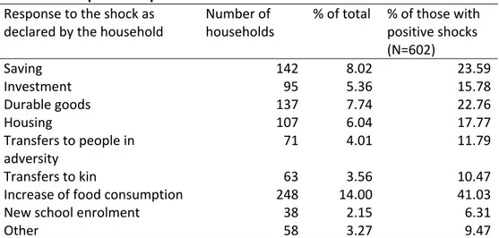
Households benefiting from these positive shocks mostly respond to it simply by increasing their food consumption (41% of those with a shock). This predominance of the food consumption response suggests highly constrained “normal” circumstances. Savings and purchase of durable goods come second with about 23% each. In 22% of the cases did households transfer extra money, either to kin or to non‐kin. Investments come last, whether productive or in the housing, and concern 15.8% and 17.8% of the responses.
Table 2 : Response to positive shocks Response to the shock as declared by the household Number of households % of total % of those with positive shocks (N=602) Saving 142 8.02 23.59 Investment 95 5.36 15.78 Durable goods 137 7.74 22.76 Housing 107 6.04 17.77 Transfers to people in adversity 71 4.01 11.79 Transfers to kin 63 3.56 10.47 Increase of food consumption 248 14.00 41.03 New school enrolment 38 2.15 6.31 Other 58 3.27 9.47 Note : Multiple answers are possible ‐ Source: PSF survey data, our own calculations. c. Bad years More households declare having suffered a negative shock than a positive one. In the case of bad years, 1005, i.e. nearly 57% of the sampled households, declare having sustained at least one exceptionally bad year in the past 5 years. More than half of those declare only one bad year (out of a maximum of 3). In the last 2 years (2005 and 2006), 628 households (35%) report a negative shock. Negative shocks are geographically even more widely distributed than positive ones, since in 80% of the clusters, at least one household declares a negative shock. Table 3: Type of negative shocks experienced by surveyed households Type of shocks Number of households % of households with negative shocks over the 5 years preceding the survey % among those with negative shocks (N=991) % of households with negative shocks in 2005/2006. Bad harvest 502 28.35 49.75 17.73 Death of livestock 150 8.47 15.04 4.23 Bad sales 179 10.11 17.76 6.38 Land loss 14 0.79 1.41 0.34 Death 155 8.75 15.24 4.12 Job loss 111 6.27 11.20 2.99 Illness 180 10.16 17.96 5.65 Divorce 23 1.30 2.22 0.39 Eviction from dwelling 23 1.30 2.32 0.62 Other 139 7.85 22.26 4.97 Note : Multiple answers are possible ‐ Source: PSF survey data, our own calculations.
The main culprit is once more to be found in agriculture with bad harvests being the most frequently named cause of bad years: in nearly 50% of the bad years is a bad harvest mentioned (see Table 3). Coming next, from the most to the least frequent, are illnesses, bad
sales, death of a household member and death of livestock. In 2005 and 2006, nearly 18% of the households declare having been subjected to a bad harvest. This is by far the most frequently reported shock (see last column).
Interestingly, here again, the most frequent response to the shock is to cope by adjusting aggregate consumption, downwards this time (Table 4).2 About 44% of households suffering a
negative shock have to resort to this decrease in consumption. The second way to cope with a blow is to borrow or obtain transfers, mainly from non‐kin, and then from kin. More than 51% of the shocks generate such a response. Table 4 also shows that about a third of the households who suffer a negative shock cope with actions that affect their future productive capacity: decrease investment, sale land, house or building, sale livestock, take a child out of school to put him to work.
A linear probability model of the probability of having faced a shock, positive or negative, confirms that rural areas witness more shocks and that households headed by an educated person and having assets, declare less adverse shocks and more favorable ones that their uneducated and asset‐less counterparts (results not shown). This is consistent with the relative frequency of agriculture related shocks documented above. Table 4: Response to negative shocks Response to the shock as declared by the household Number of households % of total % of those with negative shocks (N=991) Running savings down 157 8.87 15.74 Unpaid bills 91 5.14 9.18 Decrease consumption 446 25.18 44.6 Decrease investment 166 9.37 16.75 Land/building/house sale 19 1.07 1.92 Livestock sale 135 7.62 13.22 Durable goods sale (incl. Jewelries) 76 4.29 7.57 School dropout for work 18 1.08 1.82 New employment 63 3.56 6.26 Borrow to kin 92 5.19 9.18 Borrow to non kin 193 10.90 19.37 Transfers from kin 42 2.37 4.14 Help from non kin 183 10.33 18.37 Temporary work migration 102 5.76 10.19 Temporary migration (non work) 27 1.52 2.72 Exit of a hh member 25 1.41 2.52 Child fostered out 21 1.19 2.02 New members 15 0.85 1.51 Help from the State 15 0.85 1.51 Other 55 3.11 5.35 Note : Multiple answers are possible ‐ Source: PSF survey data, our own calculations.
2 The modalities of the response to negative shocks include "Decrease consumption" as a possible answer. However, contrary to what is the case with possible responses to positive shocks, the questionnaire does not make the distinction between adjustments in food and non food consumption.
d. Heterogeneity in shocks and responses
To end this descriptive section, we now look at the correlation between declared shocks and self‐assessed poverty, both in terms of budget constraints and in terms of access to a protective social network.
The PSF survey asks households to assess their level of economic well‐being in two ways. First, they are directly asked to which of five wealth levels they think they belong (from very poor to very rich). Second, they are also asked to think about the frequency with which they face difficulties to cover food expenditures and the probability with which they will have to face difficulties for necessary expenditures in the coming year. In addition, people are asked whether they can count on someone for help and conversely whether some people rely on them.
Only 5.8% of the sampled households think of themselves as somewhat or very rich, 6.4% think their community is rather rich. The correlation between these two assessments is 0.56. The concrete question about food expenditures indicates that 27.4% of households sometimes meet difficulties to pay for food, while 28.6% say it happens often or always. Only 36% of households declare a low risk to face difficulties with expenses in the coming year. This very high level of vulnerability is in line with the frequent adjustment in (food) consumption levels observed as response to both positive and negative shocks. Compared to others, in reaction to adverse shocks poor households are more likely to decrease consumption, to sell something, to adapt their household composition, to start working, very less likely to reduce savings. Those who have difficulties with food expenditures are the most likely to adjust household composition.
It is commonly thought that dire poverty is associated with isolation: a household who cannot rely on anyone for help is likely to be in a difficult situation. In the survey, a third of the households indicate that there is no‐one they can rely on in case of difficulties to cover necessary expenses. Conversely, 31.5% say that no‐one relies on them. The correlation between the two is 0.39, which suggests that a large number of households are really isolated, having no link in either direction.
Households who see themselves as poor are more likely to claim that no‐one relies on them (56% for the very poor, 34% for the poor, to be compared with 24% for others) and that they cannot rely on anyone (respectively 46%, 36% and 29%). For those who declare that they have frequent difficulties to face food expenses, this effect is stronger with 51% of those who always face difficulties to cover their food expenditures and 43% for those for whom it happens often, declaring they cannot count on anyone for support and respectively 64% an 42% indicating that no‐one relies on them. It is also in poor communities that households are slightly more likely to declare they are isolated (small effect).
Isolation is likely to increase poverty, especially in case of adverse shocks. Households saying they cannot rely on help are indeed less likely to benefit from transfers or loans in case of negative shocks (30% vs. 41% for connected households) and are a bit more likely to decrease their consumption (48% vs. 43%), less likely to start working and run down savings and exactly as likely to adapt their household composition. On the opposite, connected households save more often (26% vs. 18%) and make more often transfers (20% vs. 15%) in case of positive shocks.
To sum up: shocks, both positive and negative, are widespread in Senegal. The most frequently cited types of shocks are connected to key dimensions of the economic activities of households (harvests, sales, livestock). Households react to these shocks in different ways depending on their level of living standard and on the extent of their social network. Betraying the precarious situation of poor households, many of them declare that they increase food consumption when they benefit from a positive shock and decrease consumption when they are hit by an adverse one. In this case, about a third of households also resolve to adopt adjustment strategies that affect their future productive capacity: decrease investment, sale land, house or building, sale livestock, take a child out of school to put him to work. The lack of social insurance compels households to rely on the network of kin and non‐kin to get help in case of need. Poor households are however more likely to be isolated and, as such, less likely to be able to get help through loans or transfers when hit by a negative shock.
We now turn to multivariate analysis in order to, first, identify the impact of shocks on household living standards, holding into account household characteristics, and second to determine, among those characteristics, those that mitigate, or on the contrary exacerbate, the impact of shocks on household living standards.
3. Impacts of shocks on household consumption.
In what follows we examine the impact of positive and negative self declared shocks for the years 2005 and 2006 on the household level of consumption per capita during the past 12 months and on various inequality measures of intra‐household consumption. The average per capita level of consumption expenditures amounts to 640690 CFA yearly in urban areas (about 980€) and only 243220 CFA (370€) yearly in rural areas. Of these amounts, 47% go to food in urban areas while the food share reaches 66% in rural areas. While it would be preferable to use a fully exogenous measure of shocks, such as variations in the level of rainfall precipitations, this approach cannot be employed in the present case. The reason is that over the two years preceding the survey, the level of precipitations in Senegal has been close to its average over ten years. As a result, the number of households that experienced a negative rainfall shock is very low and they all belong to a small number of clusters. Since we only have cross section data, we cannot properly identify the impact of
these shocks as they confound with that of cluster fixed effects and we decided to drop this approach. a. Change in household composition in response to a shock In our setting, using per capita level of consumption as a measure of welfare creates difficulty, as households can adjust their composition in response to a shock. Therefore, comparing two apparently identical households with the same level of consumption per capita, but one having experienced a shock and not the other, could lead to the false conclusion that the shock did not have any impact. Indeed, the household having faced the shock could have coped by adjusting the number of its members. Positive shocks for instance could bring more resources to the household. Nevertheless if, as a consequence of this shock, new members join the household, consumption per capita could remain the same.
Using the same data, Abla Safir (2009) examines in great detail the impact of positive and negative shocks on entries in and departures from the household. The emerging pattern shows striking differences across rural and urban sectors, as well as across gender and age groups. What is clear nonetheless is that household composition is responsive to shocks on household well‐being.
Positive shocks tend to increase entries of young girls and adult females in rural areas. These women are not coming in to marry the household head. They are more likely to be his daughter or daughter in law. Younger girls are often grand‐daughters or have no close relation to the household head. Conversely, women entering the household in the absence of positive shocks are more likely to become wife of the head. It seems that rural households take advantage of positive shocks (or are asked by their family network) to bring in close female relatives. In urban areas, households benefiting from a positive shocks witness the arrival of additional members, mainly young adult males, maybe looking for a job. It is possible that in case of positive shocks the household is not in a position to refuse to welcome a young parent who needs a shelter in town. The resources eventually brought to the household by the positive event might then not be sufficient to cover the extra expenses occurred by the move. On the other hand, negative shocks tend to prompt departures of prime‐age adults in both rural and urban households and in particular for adult children of the household head in urban households. From this cross‐sectional data, it is difficult to know whether they were income earners before leaving or not: both situations are possible but have different implications.
Given that households can and do adjust their composition in reaction to external shocks, any estimate of the impact of shocks on household consumption per capita is likely to be downward biased. This should be kept in mind when interpreting the results that follow.
b. Determinants of household consumption
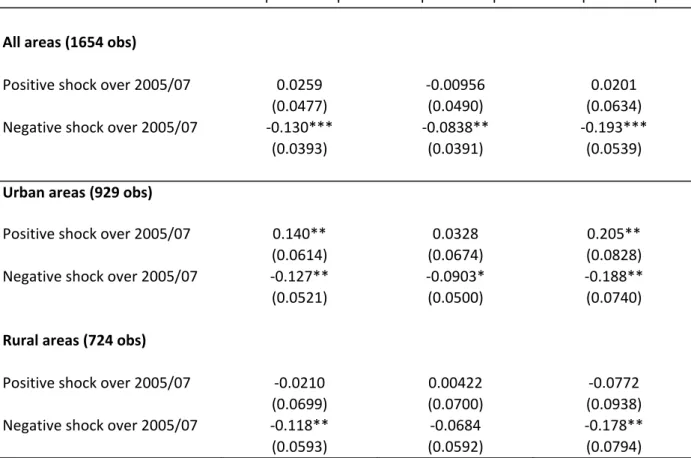
Tables A1 to A3 in the appendix show the results of linear regressions of the log household per capita annual consumption level on a set of explanatory variables, among which self declared shocks, positive and negative, over the period 2005‐2007, respectively for the whole sample and then for rural and urban areas separately3. Table 5 below shows the coefficients of the shock variables (dummy variables equal to 1 when the household declares at least on positive, resp. negative, shock) in each of these regressions. In each table, column 1 presents the regression coefficients for total per capita consumption (in logarithm), while column 2 and 3 show the results for food and non food consumption respectively.
Table 5: Impacts of shocks on household per capita consumption ‐ by area of residence ‐ selected results
(1) (2) (3)
VARIABLES Total pc consumption Food pc consumption Other pc consumption
All areas (1654 obs) Positive shock over 2005/07 0.0259 ‐0.00956 0.0201 (0.0477) (0.0490) (0.0634) Negative shock over 2005/07 ‐0.130*** ‐0.0838** ‐0.193*** (0.0393) (0.0391) (0.0539) Urban areas (929 obs) Positive shock over 2005/07 0.140** 0.0328 0.205** (0.0614) (0.0674) (0.0828) Negative shock over 2005/07 ‐0.127** ‐0.0903* ‐0.188** (0.0521) (0.0500) (0.0740) Rural areas (724 obs) Positive shock over 2005/07 ‐0.0210 0.00422 ‐0.0772 (0.0699) (0.0700) (0.0938) Negative shock over 2005/07 ‐0.118** ‐0.0684 ‐0.178** (0.0593) (0.0592) (0.0794) Robust standard errors in parentheses, *** p<0.01, ** p<0.05, * p<0.1. For full results, see tables A1 to A3. Positive (resp. negative) shock is equal to 1 is households declare at least one positive (resp. negative shock) over the period 2005‐2007.
When holding account of household characteristics, only negative shocks have a systematically significant impact on household consumption. The impact is found negative
3
and much stronger for non food (other) consumption, than for food and total consumption. In rural areas, we even observe that food consumption is left untouched in case of adverse shocks, the whole of the adjustment happening on non‐food expenses. This is what can be expected if households preserve food consumption during bad times. In urban areas only are positive shocks reflected in increased consumption, bearing entirely on non‐food products. The fact that positive shocks are not found to impact food consumption is somewhat surprising, given that in the descriptive statistics adjustment to food consumption is declared as a response to positive shocks by a large proportion of households. However, as mentioned previously, one possible explanation is that households adjust in other dimensions at the same time they increase food consumption. For instance if households bring in new members as an answer to positive shocks, then household total consumption could increase while maintaining constant consumption per capita.
Before turning to the identification of household characteristics that change the intensity of the impact of shocks, we examine the direct impact of these characteristics on household consumption, focusing on the household head's sex, marital status and education and on household composition.
Table 6 presents an excerpt of tables A1 to A3 showing the impact of marital status of the household head on consumption level by gender. Taken all together, female headed households would appear to have a higher level of consumption. This stylized fact, common to many African countries, hides a very heterogeneous reality (see van de Walle 2012). Among those women heading a household, two nearly equal sized groups have to be distinguished. The first group comprises women who are married but living independently from their husband, a fairly desirable situation possible only when either the husband is rich enough to maintain fully two households or when the wife has access to sufficient independent resources. This first situation is likely to correspond to rather richer households. A total of 176 women fit this description. The second group, of 192 unmarried women in our sample, is constituted mainly by widows and divorcees. Those are generally in a less enviable situation. The overall picture for Senegal hides important differences between urban and rural areas. In rural areas, there is very little difference according to the marital status and gender of the household head. In urban areas, the situation is different with households headed by married women having a higher consumption level than the typical household, headed by a married man. Their consumption is 18% higher. Now, the 3 groups of households: headed by men, married women and unmarried women have very different patterns of consumption, with women displaying markedly higher food consumption (around +31% for married women and 23% for unmarried ones) than men (whether married or not). Married women appear to have higher non‐food consumption (+17%) than the reference group, but the difference is not significant. Nonetheless, unmarried women display a consumption pattern that reflects a less comfortable living standard than married female household heads.
Table 6 : Impact of household head's marital status on household per capita consumption ‐ selected results
(1) (2) (3)
VARIABLES Total pc consumption Food pc consumption Other pc consumption
All areas (1653 obs) (ref group : HH married male) HH unmarried male ‐0.0506 ‐0.0914 ‐0.0628 (0.0809) (0.116) (0.101) HH married female 0.125* 0.224*** 0.129 (0.0711) (0.0721) (0.0915) HH unmarried female 0.0521 0.167** 0.0252 (0.0624) (0.0671) (0.0858) Urban areas (929 obs) (ref group : HH married male) HH unmarried male ‐0.0523 ‐0.159 0.0777 (0.103) (0.151) (0.133) HH married female 0.180* 0.310*** 0.168 (0.0956) (0.0894) (0.125) HH unmarried female 0.0817 0.226*** 0.0697 (0.0753) (0.0825) (0.101) Rural areas (724 obs) (ref group : HH married male) HH unmarried male ‐0.00863 0.0687 ‐0.231 (0.142) (0.175) (0.145) HH married female 0.0724 0.142 0.126 (0.110) (0.117) (0.143) HH unmarried female 0.0123 0.0579 ‐0.00813 (0.112) (0.113) (0.168) Robust standard errors in parentheses, *** p<0.01, ** p<0.05, * p<0.1. For full results, see tables A1 to A3. Household composition is likely to play a role as well (table 7). Household size is an obvious correlate to per capita consumption and indeed we find the expected negative effect of each group of members. Coefficients are more strongly negative for children below 5 who are certainly not contributing to household income. Now, holding household size constant, the number of cells, which gives the number of adult members having dependent individuals in charge (and therefore proxies for the number of household members with independent resources), is positively correlated with per capita expenditures, particularly so when considering non‐food consumption. Note that if we do not control for the number of cells, the negative impact of the number of adults is divided by 2 and is not significantly different from
zero for total consumption. This would reflect the fact that additional adults are potentially income earners and not only additional mouths to feed.
The type of household (nuclear, polygamous, extended non polygamous, single parent or single person)4 does not seem to have a strong impact on household consumption level. One could expect single parent families to be exposed to a higher risk of poverty, since one adult has to provide resources for the children. However, only single person households seem to have a pattern of consumption different from others, with a higher level when compared to nuclear families. This concerns mainly single men in urban areas. There is very little difference across areas so that we report in table 7 only the results on the whole sample. Note though that coefficients are stronger in urban than in rural areas. Table 7: Impacts of household composition on household per capita consumption ‐ selected results (1) (2) (3) VARIABLES Total pc consumption Food pc consumption Other pc consumption Number of adults ‐0.0326*** ‐0.0357*** ‐0.0327*** (0.00990) (0.0103) (0.0111) Number of 0‐5 years old ‐0.119*** ‐0.0949*** ‐0.138*** (0.0160) (0.0159) (0.0202) Number of 6‐15 years old ‐0.0846*** ‐0.0858*** ‐0.0806*** (0.0121) (0.0113) (0.0160) Number of cells 0.145*** 0.112*** 0.219*** (0.0299) (0.0296) (0.0370) Single parent household 0.148 0.000638 0.187 (0.0999) (0.0921) (0.144) One person household 0.561*** 0.0883 0.807*** (0.0931) (0.154) (0.124) Polygamous household 0.0541 ‐0.0699 0.135 (0.0732) (0.0710) (0.100) Extended non polygamous household ‐0.0204 ‐0.0999* 0.0501 (0.0534) (0.0542) (0.0668) Robust standard errors in parentheses, *** p<0.01, ** p<0.05, * p<0.1. For full results, see table A1. 4 Nuclear families are households composed of the head, his/her spouse, their children (biological or adopted, but not fostered), grand‐children and nephews or nieces, with no other adult. Single parent households are composed of the head of the household with his/her children (same definition as above), grand‐children, nephew or nieces with no other adult. Extended polygamous households are households in which the head lives with at least two of his wives or in which one member is the co‐spouse of the head. Extended non polygamous households include all other households, with the exception of single person households. A household made of the head, his daughter and his grand‐children is an extended household. If the mother and father of the grand‐ children are not present, the household is nuclear (unless, of course, there are other adults).
Unsurprisingly we also find that households in rural areas have a lower than average consumption level, while those with a head that has been to school at least six years fare better than average. c. Sources of heterogeneity in the impact of shocks We now look at the household characteristics that amplify or, on the contrary, dampen the impact of shocks, thereby suggesting that they contribute to risk coping possibilities. We do so by interacting key household characteristics with the positive and negative shocks variables. Interactions are tested in separate models in order to keep the results in a tractable format. For the sake of clarity, we only present the coefficients of the interaction variables in the following tables. Table 8 : Impacts of shocks on household per capita consumption ‐ by area of residence (Selected results) (1) (2) (3) VARIABLES Total pc consumption Food pc consumption Other pc consumption Rural ‐0.372*** ‐0.236*** ‐0.615*** (0.0654) (0.0624) (0.0916) Positive shock over 2005/07 0.136** 0.0289 0.197** (0.0610) (0.0663) (0.0827) Rural*(>0 shock) ‐0.193** ‐0.0647 ‐0.312** (0.0920) (0.0950) (0.123) Negative shock over 2005/07 ‐0.142*** ‐0.109** ‐0.199*** (0.0516) (0.0502) (0.0723) Rural*(<0 shock) 0.00923 0.0424 ‐0.00616 (0.0759) (0.0744) (0.103) Observations 1,653 1,653 1,653 R‐squared 0.487 0.311 0.530 Standard errors in parentheses,*** p<0.01, ** p<0.05, * p<0.1 ; Controls for household region of residence, head's sex, age, education, marital status, fostering status, religion and ethnic group, household size, household type and number of cells included. Positive (resp. negative) shock is equal to 1 is households declare at least one positive (resp. negative shock) over the period 2005‐2007. The first point we want to examine is whether households have different possibilities to cope with shocks according to their area of residence. It appears in table 8 that rural households, contrary to urban ones, do not seem to be able to benefit from positive shocks in terms of per capita consumption. It could be due to many reasons. A hypothesis to be explored is that it reflects the taxing away of any supplementary income by the solidarity duties towards one’s network. As mentioned above, Abla Safir (2009) shows that shocks are often followed by changes in family structure, and in particular, for rural households, by new entries of female members, that could be a form of redistribution. By contrast, prime‐age adult males tend to join urban households in case of positive shocks and the result below suggest either that they
might have a positive contribution to household income, or that they do not absorb the whole of the extra income linked to the shock.
An attempt was made at exhibiting differences between ethnic groups. For the most part, interactions between the shock variables and the ethnic group of the household do not have a statistically significant impact on consumption level. There are few exceptions (7 out of 42 coefficients) but they seem nearly random and have no clear interpretation. Table 9: Impacts of shocks on household per capita consumption ‐ by head's education level (Selected results) (1) (2) (3) VARIABLES Total pc consumption Food pc consumption Other pc consumption HHead educ. 4‐5 years ‐0.0342 0.00475 0.00667 (0.0720) (0.0753) (0.101) HHead educ. 6‐9 years 0.269*** 0.241*** 0.379*** (0.0883) (0.0880) (0.117) HHead educ. >= 10 years 0.395*** 0.295*** 0.582*** (0.0887) (0.104) (0.114) HHead koranic schooling 0.0312 0.0625 0.0609 (0.0608) (0.0617) (0.0827) Positive shock over 2005/07 ‐0.00330 0.00747 ‐0.105 (0.0775) (0.0811) (0.0990) (HHead educ 4‐5y)*(>0 shock) 0.0458 ‐0.143 0.360 (0.159) (0.150) (0.236) (HHead educ 6‐9 y)*(>0 shock) ‐0.131 0.0590 ‐0.254 (0.146) (0.153) (0.192) (HHead educ >= 10 y)*(>0 shock) 0.145 0.0328 0.279 (0.158) (0.157) (0.222) (HHead edcoran)*(>0 shock) 0.0636 ‐0.0204 0.253* (0.111) (0.116) (0.144) Negative shock over 2005/07 ‐0.162*** ‐0.0957 ‐0.193** (0.0593) (0.0600) (0.0776) (HHead educ 4‐5y)*(<0 shock) 0.160 0.230* ‐0.0962 (0.132) (0.130) (0.195) (HHead educ 6‐9 y)*(<0 shock) 0.0198 ‐0.144 0.0597 (0.161) (0.145) (0.195) (HHead educ >= 10 y)*(<0 shock) 0.213* 0.0301 0.190 (0.125) (0.165) (0.184) (HHead edcoran)*(<0 shock) 0.00947 ‐0.00443 ‐0.0203 (0.0889) (0.0879) (0.118) Observations 1,653 1,653 1,653 R‐squared 0.487 0.313 0.531 Standard errors in parentheses ; *** p<0.01, ** p<0.05, * p<0.1 ; Controls for household area and region of residence, head's sex, age, marital status, fostering status, religion and ethnic group, household size, household type and number of cells included. Positive (resp. negative) shock is equal to 1 is households declare at least one positive (resp. negative shock) over the period 2005‐2007.
We do not find either any strong impact of education (see table 9). Although households with highly educated heads have a higher level of consumption, they do not appear better able to resist negative shocks than uneducated ones. This is not what is expected if one assumes that educated heads are more likely to have better access to social protection and credit market.
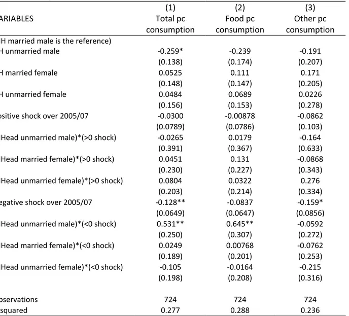
Table 10 : Impacts of shocks on household per capita consumption ‐ by head's sex and marital status (Selected results for rural areas) (1) (2) (3) VARIABLES Total pc consumption Food pc consumption Other pc consumption (HH married male is the reference) HH unmarried male ‐0.259* ‐0.239 ‐0.191 (0.138) (0.174) (0.207) HH married female 0.0525 0.111 0.171 (0.148) (0.147) (0.205) HH unmarried female 0.0484 0.0689 0.0226 (0.156) (0.153) (0.278) Positive shock over 2005/07 ‐0.0300 ‐0.00878 ‐0.0862 (0.0789) (0.0786) (0.103) (HHead unmarried male)*(>0 shock) ‐0.0265 0.0179 ‐0.164 (0.391) (0.367) (0.633) (HHead married female)*(>0 shock) 0.0451 0.131 ‐0.0868 (0.230) (0.227) (0.343) (HHead unmarried female)*(>0 shock) 0.0804 0.0322 0.276 (0.203) (0.214) (0.334) Negative shock over 2005/07 ‐0.128** ‐0.0837 ‐0.159* (0.0649) (0.0647) (0.0856) (HHead unmarried male)*(<0 shock) 0.531** 0.645** ‐0.0592 (0.250) (0.307) (0.272) (HHead married female)*(<0 shock) 0.0249 0.00768 ‐0.0762 (0.189) (0.201) (0.253) (HHead unmarried female)*(<0 shock) ‐0.105 ‐0.0164 ‐0.215 (0.198) (0.208) (0.316) Observations 724 724 724 R‐squared 0.277 0.288 0.236 Standard errors in parentheses, *** p<0.01, ** p<0.05, * p<0.1; Controls for household area and region of residence, head's age, education, fostering status, religion and ethnic group, household size, household type and number of cells included. Positive (resp. negative) shock is equal to 1 is households declare at least one positive (resp. negative shock) over the period 2005‐2007.
Tables 10 and 11 show the results obtained regarding the role of the gender of the head of household. As seen above, marital status matters differently for male and female household heads. We therefore look at the role of gender interacted with marital status. One could expect to find some heterogeneity in the ability to resist negative shocks or to benefit from positive ones depending on the head's sex, if for instance household headed by widowed women are more likely to be poor or socially disconnected. We indeed find that consumption
of households headed by married female benefit less from positive shocks than their male counterpart in urban areas (table 11), but this is mainly due to the fact that the few women in this situation tend to take advantage of positive shocks to invest in a house. In rural areas, only households headed by unmarried males appear to fare better than others when hit by an adverse shock, but this concerns a very small set of households (10).
Table 11 : Impacts of shocks on household per capita consumption ‐ by head's sex and marital status (Selected results for urban areas) (1) (2) (3) VARIABLES Total pc consumption Food pc consumption Other pc consumption (HH married male is the reference) HH unmarried male ‐0.0786 0.000986 ‐0.0355 (0.106) (0.168) (0.138) HH married female 0.269** 0.370*** 0.254* (0.109) (0.0998) (0.142) HH unmarried female 0.118 0.218** 0.152 (0.0937) (0.0999) (0.118) Positive shock over 2005/07 0.142** 0.0641 0.175* (0.0676) (0.0839) (0.0919) (HHead unmarried male)*(>0 shock) 0.395 ‐0.249 0.790** (0.258) (0.310) (0.319) (HHead married female)*(>0 shock) ‐0.465*** ‐0.313* ‐0.493* (0.177) (0.163) (0.266) (HHead unmarried female)*(>0 shock) 0.0944 0.137 0.117 (0.199) (0.164) (0.254) Negative shock over 2005/07 ‐0.0791 ‐0.0420 ‐0.126 (0.0620) (0.0604) (0.0863) (HHead unmarried male)*(<0 shock) ‐0.183 ‐0.584* ‐0.0681 (0.253) (0.303) (0.298) (HHead married female)*(<0 shock) ‐0.126 ‐0.0789 ‐0.0964 (0.188) (0.150) (0.253) (HHead unmarried female)*(<0 shock) ‐0.187 ‐0.0481 ‐0.352* (0.120) (0.118) (0.194) Observations 929 929 929 R‐squared 0.400 0.256 0.394 Standard errors in parentheses,*** p<0.01, ** p<0.05, * p<0.1 ; Controls for household area and region of residence, head's age, education, fostering status, religion and ethnic group, household size, household type and number of cells included. Positive (resp. negative) shock is equal to 1 is households declare at least one positive (resp. negative shock) over the period 2005‐2007.
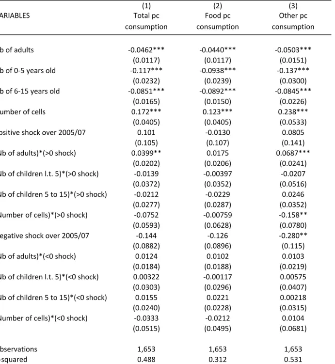
When looking at whether household composition matters in the ability to cope with shocks (table 12), not much appears, apart that households with a larger number of adults benefit more from positive shocks, increasing their per capita non‐food consumption level by 4% percent per additional adult member in case of positive shock. This is nevertheless only sufficient to compensate for the average disadvantage (of nearly ‐4.6% per additional adult member but ‐8% or 12% per additional child, depending on age group) of bigger households.
The number of cells is found negatively associated to the ability to increase non food consumption in case of a positive shock, which could result from the fact that an additional cell implies both an additional adult and some dependents. Hence, taken together with the impact of additional adult member, this result suggests that an additional adult member who comes alone in the household is a resource that allows taking advantage of positive shocks but if the adult comes with dependents, this prevents the positive shocks to translate into significant per capita consumption gains.
Table 12: Impacts of shocks on household per capita consumption ‐ by household size (Selected results) (1) (2) (3) VARIABLES Total pc consumption Food pc consumption Other pc consumption Nb of adults ‐0.0462*** ‐0.0440*** ‐0.0503*** (0.0117) (0.0117) (0.0151) Nb of 0‐5 years old ‐0.117*** ‐0.0938*** ‐0.137*** (0.0232) (0.0239) (0.0300) Nb of 6‐15 years old ‐0.0851*** ‐0.0892*** ‐0.0845*** (0.0165) (0.0150) (0.0226) Number of cells 0.172*** 0.123*** 0.238*** (0.0405) (0.0405) (0.0533) Positive shock over 2005/07 0.101 ‐0.0130 0.0805 (0.105) (0.107) (0.141) (Nb of adults)*(>0 shock) 0.0399** 0.0175 0.0687*** (0.0202) (0.0206) (0.0241) (Nb of children l.t. 5)*(>0 shock) ‐0.0139 ‐0.00397 ‐0.0207 (0.0372) (0.0352) (0.0516) (Nb of children 5 to 15)*(>0 shock) ‐0.0212 ‐0.0229 0.0246 (0.0277) (0.0287) (0.0352) (Number of cells)*(>0 shock) ‐0.0752 ‐0.00759 ‐0.158** (0.0593) (0.0628) (0.0780) Negative shock over 2005/07 ‐0.144 ‐0.126 ‐0.280** (0.0882) (0.0896) (0.115) (Nb of adults)*(<0 shock) 0.0124 0.0102 0.0103 (0.0184) (0.0188) (0.0219) (Nb of children l.t. 5)*(<0 shock) 0.00322 ‐0.00117 0.00575 (0.0303) (0.0296) (0.0407) (Nb of children 5 to 15)*(<0 shock) 0.0155 0.0221 0.00218 (0.0240) (0.0228) (0.0315) (Number of cells)*(<0 shock) ‐0.0333 ‐0.0212 0.0104 (0.0515) (0.0495) (0.0681) Observations 1,653 1,653 1,653 R‐squared 0.488 0.312 0.531 Standard errors in parentheses,*** p<0.01, ** p<0.05, * p<0.1 ; Controls for household area and region of residence, head's age, education, marital status, fostering status, religion and ethnic group, household type included. Positive (resp. negative) shock is equal to 1 is households declare at least one positive (resp. negative shock) over the period 2005‐2007.
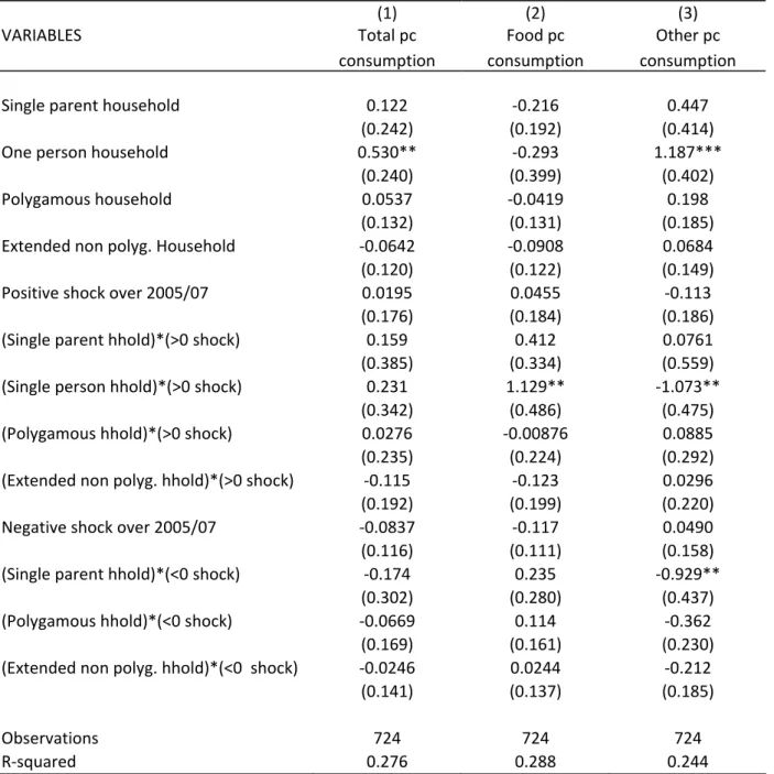
Tables 13 and 14 show the heterogeneous impact of shocks depending on the type of household in urban and rural areas respectively. Though the household type does not seem to impact much the household consumption level, it seems that it modifies the impact of either positive or negative shocks. Interestingly we find that extended, non polygamous, households appear to be better able to resist to negative shocks in urban areas. Table 13 : Impacts of shocks on household per capita consumption ‐ by household type (Selected results for urban areas) (1) (2) (3) VARIABLES Total pc consumption Food pc consumption Other pc consumption Single parent household 0.121 0.0713 0.0684 (0.143) (0.114) (0.200) One person household 0.530*** 0.248 0.541*** (0.121) (0.198) (0.159) Polygamous household 0.176 ‐0.220* 0.299 (0.147) (0.123) (0.200) Extended non polyg. household ‐0.0305 ‐0.120 ‐0.0384 (0.0780) (0.0756) (0.102) Positive shock over 2005/07 0.0954 0.167* ‐0.0161 (0.0999) (0.0960) (0.147) (Single parent hhold)*(>0 shock) 0.353 ‐0.0713 0.586 (0.329) (0.250) (0.464) (Single person hhold)*(>0 shock) ‐0.0169 ‐0.779* 0.476 (0.250) (0.400) (0.296) (Polygamous hhold)*(>0 shock) ‐0.156 ‐0.0110 ‐0.0647 (0.250) (0.234) (0.334) (Extended non polyg. hhold)*(>0 shock) 0.0396 ‐0.126 0.243 (0.123) (0.126) (0.174) Negative shock over 2005/07 ‐0.261*** ‐0.137* ‐0.389*** (0.0927) (0.0832) (0.131) (Single parent hhold)*(<0 shock) ‐0.00477 ‐0.110 0.0204 (0.187) (0.191) (0.305) (Single person hhold)*(<0 shock) 0.411 0.315 0.485 (0.271) (0.330) (0.335) (Polygamous hhold)*(<0 shock) ‐0.0845 0.187 ‐0.133 (0.218) (0.203) (0.295) (Extended non polyg. hhold)*(<0 shock) 0.229** 0.0681 0.335** (0.114) (0.106) (0.162) Observations 929 929 929 R‐squared 0.400 0.258 0.394 Standard errors in parentheses,*** p<0.01, ** p<0.05, * p<0.1 ; Controls for household area and region of residence, head's age, education, marital status, fostering status, religion and ethnic group, household size and number of cells included. Positive (resp. negative) shock is equal to 1 is households declare at least one positive (resp. negative shock) over the period 2005‐2007.
On the opposite, in rural areas single parent households appear to suffer much more from adverse shocks than nuclear families. These results are to be expected if extended households have a higher ability to obtain external support in case of difficulties, due to a larger social network. Single parent households are more likely to be isolated. However these results are not corroborated when we analyze the household network impact: households who declare they can get help in case of need do not appear better protected from negative shocks (results not shown).
Table 14 : Impacts of shocks on household per capita consumption ‐ by household type (Selected results for rural areas) (1) (2) (3) VARIABLES Total pc consumption Food pc consumption Other pc consumption Single parent household 0.122 ‐0.216 0.447 (0.242) (0.192) (0.414) One person household 0.530** ‐0.293 1.187*** (0.240) (0.399) (0.402) Polygamous household 0.0537 ‐0.0419 0.198 (0.132) (0.131) (0.185) Extended non polyg. Household ‐0.0642 ‐0.0908 0.0684 (0.120) (0.122) (0.149) Positive shock over 2005/07 0.0195 0.0455 ‐0.113 (0.176) (0.184) (0.186) (Single parent hhold)*(>0 shock) 0.159 0.412 0.0761 (0.385) (0.334) (0.559) (Single person hhold)*(>0 shock) 0.231 1.129** ‐1.073** (0.342) (0.486) (0.475) (Polygamous hhold)*(>0 shock) 0.0276 ‐0.00876 0.0885 (0.235) (0.224) (0.292) (Extended non polyg. hhold)*(>0 shock) ‐0.115 ‐0.123 0.0296 (0.192) (0.199) (0.220) Negative shock over 2005/07 ‐0.0837 ‐0.117 0.0490 (0.116) (0.111) (0.158) (Single parent hhold)*(<0 shock) ‐0.174 0.235 ‐0.929** (0.302) (0.280) (0.437) (Polygamous hhold)*(<0 shock) ‐0.0669 0.114 ‐0.362 (0.169) (0.161) (0.230) (Extended non polyg. hhold)*(<0 shock) ‐0.0246 0.0244 ‐0.212 (0.141) (0.137) (0.185) Observations 724 724 724 R‐squared 0.276 0.288 0.244 Standard errors in parentheses,*** p<0.01, ** p<0.05, * p<0.1 ; Controls for household area and region of residence, head's age, education, fostering status, marital status, religion and ethnic group, household size and number of cells included. Positive (resp. negative) shock is equal to 1 is households declare at least one positive (resp. negative shock) over the period 2005‐2007.
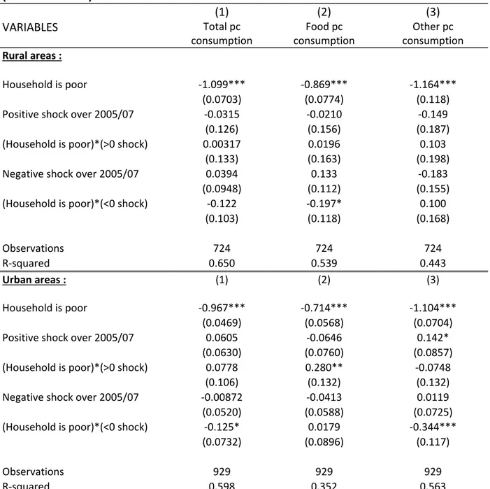
We finally examine the impact of household poverty and total assets. We expect that poor households have less possibility to smooth consumption in case of shocks. Conversely household assets should help. Indeed, for households with some savings capacity we expect negative and positive shocks to have a smaller impact on consumption: in good years, the household is expected to save, while in bad years it is expected to reduce its savings.
Table 15: Impacts of shocks on household per capita consumption ‐ by poverty status (Selected results) (1) (2) (3) VARIABLES Total pc consumption Food pc consumption Other pc consumption Rural areas : Household is poor ‐1.099*** ‐0.869*** ‐1.164*** (0.0703) (0.0774) (0.118) Positive shock over 2005/07 ‐0.0315 ‐0.0210 ‐0.149 (0.126) (0.156) (0.187) (Household is poor)*(>0 shock) 0.00317 0.0196 0.103 (0.133) (0.163) (0.198) Negative shock over 2005/07 0.0394 0.133 ‐0.183 (0.0948) (0.112) (0.155) (Household is poor)*(<0 shock) ‐0.122 ‐0.197* 0.100 (0.103) (0.118) (0.168) Observations 724 724 724 R‐squared 0.650 0.539 0.443 Urban areas : (1) (2) (3) Household is poor ‐0.967*** ‐0.714*** ‐1.104*** (0.0469) (0.0568) (0.0704) Positive shock over 2005/07 0.0605 ‐0.0646 0.142* (0.0630) (0.0760) (0.0857) (Household is poor)*(>0 shock) 0.0778 0.280** ‐0.0748 (0.106) (0.132) (0.132) Negative shock over 2005/07 ‐0.00872 ‐0.0413 0.0119 (0.0520) (0.0588) (0.0725) (Household is poor)*(<0 shock) ‐0.125* 0.0179 ‐0.344*** (0.0732) (0.0896) (0.117) Observations 929 929 929 R‐squared 0.598 0.352 0.563 Standard errors in parentheses, *** p<0.01, ** p<0.05, * p<0.1; Controls for household area and region of residence, head's sex, age, education, marital status, fostering status, religion and ethnic group, household size, household type and number of cells included ‐ household is poor if per capita consumption level is lower than median. Positive (resp. negative) shock is equal to 1 is households declare at least one positive (resp. negative shock) over the period 2005‐2007. We find indeed that households whose consumption per capita is below the median diminish their consumption more than richer households in case of negative shock (table 15). In rural areas, the brunt of the differential adjustment is borne by food consumption (‐20%), while in
urban areas poor households reduce their non‐food consumption by 34% more than non‐poor ones. We also observe that in case of a positive shock, in urban areas, only poor households increase significantly their food consumption level (+28%), betraying once again the precarious situation of those households.
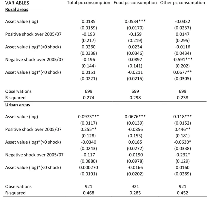
Finally, as shown in table 16 below, we find unsurprisingly that assets are positively related to household consumption. In line with what was expected, the impact of positive (in urban areas) and negative shocks (in rural areas) is smaller the larger the level of assets owned by the household. This confirms the role of assets as a buffer stock that helps household to smooth their consumption.
Table 16: Impacts of shocks on household per capita consumption ‐ by assets level (selected results)
(1) (2) (3)
VARIABLES Total pc consumption Food pc consumption Other pc consumption
Rural areas Asset value (log) 0.0185 0.0534*** ‐0.0332 (0.0159) (0.0170) (0.0237) Positive shock over 2005/07 ‐0.193 ‐0.159 0.0147 (0.217) (0.219) (0.295) Asset value (log)*(>0 shock) 0.0260 0.0234 ‐0.0116 (0.0338) (0.0346) (0.0434) Negative shock over 2005/07 ‐0.196 0.0897 ‐0.591*** (0.144) (0.141) (0.202) Asset value (log)*(<0 shock) 0.0151 ‐0.0211 0.0677** (0.0221) (0.0215) (0.0305) Observations 699 699 699 R‐squared 0.274 0.298 0.238 Urban areas Asset value (log) 0.0973*** 0.0676*** 0.118*** (0.0117) (0.0139) (0.0152) Positive shock over 2005/07 0.255** ‐0.0856 0.446** (0.128) (0.153) (0.181) Asset value (log)*(>0 shock) ‐0.0340 0.0185 ‐0.0630* (0.0243) (0.0272) (0.0338) Negative shock over 2005/07 ‐0.117 ‐0.0190 ‐0.232* (0.0880) (0.0978) (0.129) Asset value (log)*(<0 shock) 0.000270 ‐0.0166 0.0160 (0.0191) (0.0202) (0.0269) Observations 921 921 921 R‐squared 0.468 0.285 0.452 Standard errors in parentheses, *** p<0.01, ** p<0.05, * p<0.1 ; Controls for household area and region of residence, head's sex, age, education, marital status, fostering status, religion and ethnic group, household size, household type and number of cells included. Positive (resp. negative) shock is equal to 1 is households declare at least one positive (resp. negative shock) over the period 2005‐2007.
4. Inequalities within households
The measurement of cell consumption levels allows studying the determinants of intra‐ household inequalities and how these are modified in the event of a shock. In what follows, two inequality measures have been considered: first we have computed, for each household, the within household coefficient of variation of cell per capita consumption levels. We then consider as being highly unequal those households for which the coefficient of variation belongs to the highest quartile of the coefficient distribution. Second, for each cell we compute the value of its per capita consumption level as a proportion of the maximum per capita consumption level within the household. a. Characteristics of highly unequal households
The average intra‐household coefficient of variation of cell per capita consumption (when there is more than one cell in the household) is equal to 0.29. According to this measure, the level of inequality is much higher for non‐food consumption than it is for food consumption: 0.55 versus 0.04. Hence, most of the within household inequality is concentrated on non‐food consumption, in line with traditional obligations made to household heads to provide for necessities of household members.
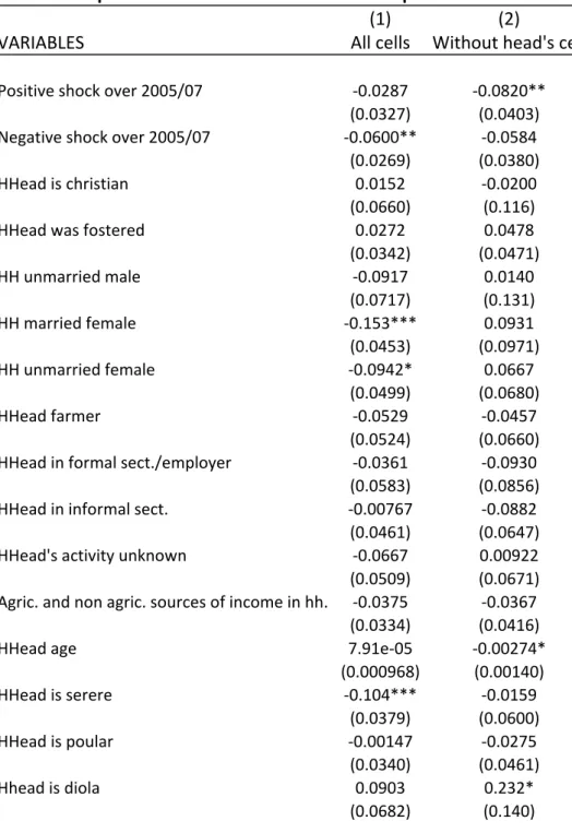
We begin by examining the determinants of intra‐household inequality. Our measure of inequality is a dummy variable that equals 1 if the household is among the 25% most unequal households, based on the coefficient of variation of cell per capita consumption level within the household.5 Table 17 shows the determinants of that inequality measure, using a linear probability model. Only those households with at least two cells are included in the regression. In column (1) we present the results keeping all cells in the analysis. In column (2) we report the results obtained when considering only inequality between cells other than that of the head. This further reduces the sample to households that are constituted of at least three cells. Indeed, the specific role of the household head implies that he takes charge of a number of expenditures that in reality might benefit the whole household. Comparing non‐ head cells might give a different picture than comparing head to non‐head.
Looking at the top part of the table we see that adverse shocks have a significant negative impact on intra‐household inequalities (excluding the cell of the household head, the coefficient is very similar but only verging on significance). Positive shocks have the same impact, but it is only significant in the second column, when we exclude the household head's cell. Interestingly we find that households headed by a female are less likely to be very unequal. But this effect is found only when we compare the head's cell consumption level
5
with that of other cells. When the head's cell is excluded this effect vanishes. This suggests that the lower level of inequality within female headed households comes from a relatively lower level of consumption of the head's cell compared to other cells, hence maybe from a lesser capture of resources by the household head when the household is female headed. A higher number of cells is associated with more inequality, maybe due to the multiplication of independent sources of income. In the same vein, we also observe that polygamous households are more likely to be unequal, but this effect disappears once the head's cell is dropped from the analysis, suggesting that inequality is higher between the head's cell and those of his wives than between wives' cells.
Table 17: Impact of shocks on intrahousehold inequalities
(1) (2)
VARIABLES All cells Without head's cell
Positive shock over 2005/07 ‐0.0287 ‐0.0820** (0.0327) (0.0403) Negative shock over 2005/07 ‐0.0600** ‐0.0584 (0.0269) (0.0380) HHead is christian 0.0152 ‐0.0200 (0.0660) (0.116) HHead was fostered 0.0272 0.0478 (0.0342) (0.0471) HH unmarried male ‐0.0917 0.0140 (0.0717) (0.131) HH married female ‐0.153*** 0.0931 (0.0453) (0.0971) HH unmarried female ‐0.0942* 0.0667 (0.0499) (0.0680) HHead farmer ‐0.0529 ‐0.0457 (0.0524) (0.0660) HHead in formal sect./employer ‐0.0361 ‐0.0930 (0.0583) (0.0856) HHead in informal sect. ‐0.00767 ‐0.0882 (0.0461) (0.0647) HHead's activity unknown ‐0.0667 0.00922 (0.0509) (0.0671) Agric. and non agric. sources of income in hh. ‐0.0375 ‐0.0367 (0.0334) (0.0416) HHead age 7.91e‐05 ‐0.00274* (0.000968) (0.00140) HHead is serere ‐0.104*** ‐0.0159 (0.0379) (0.0600) HHead is poular ‐0.00147 ‐0.0275 (0.0340) (0.0461) Hhead is diola 0.0903 0.232* (0.0682) (0.140)