HAL Id: hal-01997352
https://hal.utc.fr/hal-01997352
Submitted on 5 Feb 2019
HAL is a multi-disciplinary open access archive for the deposit and dissemination of sci-entific research documents, whether they are pub-lished or not. The documents may come from teaching and research institutions in France or abroad, or from public or private research centers.
L’archive ouverte pluridisciplinaire HAL, est destinée au dépôt et à la diffusion de documents scientifiques de niveau recherche, publiés ou non, émanant des établissements d’enseignement et de recherche français ou étrangers, des laboratoires publics ou privés.
To cite this version:
Xuan Do, Adnan Ibrahimbegovic. 2D continuum viscodamage-embedded discontinuity model with second order mid-point scheme. Coupled systems mechanics, Techno-Press, 2018, 7, pp.669 - 690. �10.12989/csm.2018.7.6.669�. �hal-01997352�
Copyright © 2018 Techno-Press, Ltd.
http://www.techno-press.org/?journal=csm&subpage=8 ISSN: 2234-2184 (Print), 2234-2192 (Online)
2D continuum viscodamage-embedded discontinuity model
with second order mid-point scheme
Xuan Nam Do
*and Adnan Ibrahimbegovic
aUniversité de Technologie Compiègne / Sorbonne Universités, Laboratoire Roberval de Mécanique Centre de Recherche Royallieu, Rue Personne de Roberval, 60200 Compiègne, France
(Received Augst 1, 2018, Revised September 3, 2018, Accepted September 4, 2018)
Abstract. This paper deals with numerical modeling of dynamic failure phenomena in rate-sensitive brittle and/or ductile materials. To this end, a two-dimensional continuum viscodamage-embedded discontinuity model, which is based on our previous work (see Do et al. 2017), is developed. More specifically, the pre-peak nonlinear and rate-sensitive hardening response of the material behavior, representing the fracture-process zone creation, is described by a rate-dependent continuum damage model. Meanwhile, an embedded displacement discontinuity model is used to formulate the post-peak response, involving the macro-crack creation accompanied by exponential softening. The numerical implementation in the context of the finite element method exploiting the second-order mid-point scheme is discussed in detail. In order to show the performance of the model several numerical examples are included.
Keywords: dynamics; fracture process zone-FPZ; strain-softening; localization; finite element; embedded discontinuity; mid-point scheme
1. Introduction
According to Cervera et al. (1995): “As it is well known, brittle materials, especially concrete exhibit a rate-dependent behavior when subjected to high rate straining with significant increase of dynamic strengths and decrease of nonlinearity on the stress-strain response curves, when compared to those measured in static tests. Observational experience shows that rate sensitivity is primarily due to the fact that the growth of internal micro-cracking is retarded at high strain rate”. This characteristic of strong strain-rate sensitivity of brittle materials together with the presence of inertia effects cause principal modeling difficulties in the field of numerical simulation of crack propagation and localized failure analyses of structures and structural components under dynamic loading.
Starting from the observed evidence that this particular behavior is in fact consequence of the strain-rate dependency of the internal damage evolution, several rate-dependent continuum damage models were proposed concerning micro-crack interaction and growth under dynamic loading (e.g., Grady and Kipp 1980, Suaris and Shah 1984, Taylor et al. 1986, Fahrenthold 1991,
Corresponding author, Ph.D., E-mail: [email protected]
Fig. 1 The discontinuity surface Г𝑠 separating the domain into + and −and strong discontinuity
kinematics
Fig. 2 Discontinuous shape function (2D case) for a CST element with constant discontinuity jumps
Yang et al. 1996, Yazdchi et al. 1996, Lu and Xu 2004, Wang et al. 2008, Hamdi et al. 2011). Even though the ill-posed problem due to strain softening, which is the source of major problems such as spurious mesh dependency, mesh alignment effects (De Borst et al. 1993) and failure without energy dissipation (Bažant 1976), can be avoided when rate-dependent constitutive relations are implemented carefully most of such continuum mechanics-based models, however, are not suitable to correctly predict damage localization processes where strain-softening phenomenon appears (see Bažant et al. 1984, Needleman 1988).
To avoid the problem outlined above the introduction of a localization limiter is required. One of the most promising relatively recent techniques for finite element modeling of crack propagation which can be employed for this purpose is the embedded strong discontinuity approach, in which the displacement field is enhanced to capture the discontinuity (crack) (e.g., Simo et al. 1993, Armero and Garikipati 1995, Oliver 1996, Oliver 2000, Alfaiate et al. 2002, Huespe et al. 2006, Ibrahimbegovic and Melnyk 2007, Linder and Armero 2007, Armero and Linder 2009, Brancherie and Ibrahimbegovic 2009, Radulovic et al. 2011, Dujc et al. 2013, Saksala et al. 2015), leading to a regularization of the modeling of reality. As the main novelty, herein we present a two-dimensional continuum viscodamage-embedded discontinuity model. This model concentrates on dynamic fracture, with an emphasis on crack phenomena, by using the
mid-point rule in order to carry out the time-integration for such a problem in each time step. The outline of the paper is as follows: First, the theoretical formulation is briefly presented in
Section 2. Next, Section 3 is devoted to numerical implementation where computational procedure is given in full detail, followed by Section 4 in which numerical simulations are performed and analyzed. Finally, some conclusions are drawn in Section 5.
2. Theoretical formulation
2.1 Rate-dependent continuum damage model
The internal energy of such a damage model can formally be written
̅(𝛆̅, 𝐃̅ , 𝜉̅) =1 2𝛆̅ • 𝐃̅
−𝟏𝛆̅ + Ξ̅(𝜉̅) (1)
where 𝜉̅ is the hardening variable, and Ξ̅(𝜉̅) stands for the corresponding hardening potential. The damage function is defined by
Ф̅ (𝛔, 𝑞̅) = Ф̅̂ (𝛔) − (𝜎̅𝑓− 𝑞̅) (2)
where 𝜎̅𝑓 refers to the limit of elasticity indicating the first cracking and 𝑞̅ is a stress-like
hardening variable which handles the damage threshold evolution.
By using the Legendre transformation to exchange the roles between the stress and deformation, we further introduce the complementary energy potential
̅(𝛔, 𝐃̅ , 𝜉̅) = 𝛔 • 𝛆̅ −̅(𝛆̅, 𝐃̅ , 𝜉̅) =1
2𝛔 • 𝐃̅ 𝛔 − Ξ̅(𝜉̅) (3)
By exploiting the second law of thermodynamics, we can obtain the explicit form of the damage model dissipation defined as follows
0 ≤ 𝒟̅ = 𝛔 • 𝛆̅̇ −̅̇(𝛆̅, 𝐃̅ , 𝜉̅) = 𝛔̇(−𝛆̅ + 𝐃̅ 𝛔) +1
2𝛔 • 𝐃̅̇ 𝛔 − 𝑑Ξ̅(𝜉̅)
𝑑𝜉̅ 𝜉̅̇ (4)
In the case of “elastic” process where 𝐃̅̇ = 0 and 𝜉̅̇ = 0 , the dissipation inequality (the Clausius-Duhem inequality) above becomes an equality with 𝒟̅ = 0. This leads to the appropriate form of constitutive equations for damage model
𝛔̇(−𝛆̅ + 𝐃̅ 𝛔) = 0 ⟺ 𝛆̅ = 𝐃̅ 𝛔 ⟹ 𝛔 = 𝐃̅−𝟏𝛆̅ = 𝜕̅(𝛆̅, 𝐃̅ , 𝜉̅)
𝜕𝛆̅ ; 𝑞̅ = − 𝑑Ξ̅(𝜉̅)
𝑑𝜉̅ (5)
By assuming that these equations remain valid for an inelastic process with 𝐃̅̇ ≠ 0; 𝜉̅̇ ≠ 0, we can redefine the damage dissipation
0 < 𝒟̅ =1 2𝛔 • 𝐃̅̇ 𝛔 − 𝑑Ξ̅(𝜉̅) 𝑑𝜉̅ 𝜉̅̇ = 1 2𝛔 • 𝐃̅̇ 𝛔 + 𝑞̅𝜉̅̇ (6)
Here in order to seek the best formulation for high-order scheme such as the mid-point, we introduce the main novelty of using the viscous regularization of damage, leading to visco-damage. This is obtained by using the regularized maximum dissipation to enforce the constraint Ф̅ (𝛔, 𝑞̅) ≤ 0. Such form of the damage model is capable of taking into account rate-sensitivity of the response and it is further referred as visco-damage. To that end, the problem can be recast as the unconstrained maximization problem
max
Ф̅ (𝛔,𝑞̅)≤0[𝒟̅(𝛔, 𝑞̅)] ⟺ max𝛾̅̇≥0 ∀(𝛔,𝑞̅)min [−𝒟⏟ ̅(𝛔, 𝐃̅ , 𝜉̅) + 𝑃̅(Ф̅ (𝛔, 𝑞̅))]
ℒ̅(𝛔,𝐃̅ ,𝜉̅,𝑞̅) (7)
where 𝑃̅(Ф̅ (𝛔, 𝑞̅), a quadratic form of the penalty term, is defined by 𝑃̅(Ф̅ (𝛔, 𝑞̅)) = { 1 2̅Ф̅ 2; Ф̅ > 0 0; Ф̅ ≤ 0 (8)
where ̅ is the viscosity parameter for continuum damage model.
By applying the Kuhn-Tucker optimality conditions for the chosen damage Lagrangian the evolution equations for the internal variables can thus be written
0 =∂ℒ̅(𝛔, 𝐃𝛔̅ , 𝜉̅, 𝑞̅)= −𝐃̅̇ 𝛔 +〈Ф̅ 〉 ̅ Ф̅ (𝛔, 𝑞̅) 𝛔 0 =∂ℒ̅(𝛔, 𝐃̅ , 𝜉̅, 𝑞̅) ∂𝑞̅ = −𝜉̅̇ + 〈Ф̅ 〉 ̅ Ф̅ (𝛔, 𝑞̅) ∂𝑞̅ (9)
where symbol <∙> denotes the Macauley parenthesis, which will filter out only the positive value of its argument.
For Ф̅̂ (𝛔), a homogeneous function of degree one, implies that Ф𝛔̅𝛔 = Ф̅̂ (𝛔), we can rewrite (9)1 as 𝐃̅̇ =〈Ф̅ 〉 ̅ 1 Ф̅̂ (𝛔) Ф̅ 𝛔 ⊗ Ф̅ 𝛔 (10)
By introducing the new definition of damage multiplier 𝛾̅̇ =〈Ф̅ 〉̅ , the evolution equation for rate-sensitive damage model in (9) can be recast in standard format as
𝐃 ̅̇ = 𝛾̅̇ 1 Ф̅̂ (𝛔) Ф̅ 𝛔⊗ Ф̅ 𝛔 𝜉̅̇ = 𝛾̅̇Ф̅ 𝛔 (11)
We note that the damage multiplier can be directly computed from the current (positive) value of damage function. From there, for the isotropic case, damage model is characterized by
Ф̅ (𝛔, 𝑞̅) = √𝛔 • 𝐃⏟ e𝛔 ‖𝛔‖𝐃𝑒 − 1 √𝐸(𝜎̅𝑓− 𝑞̅); 𝛾̅̇ = 〈Ф̅ (𝛔, 𝑞̅)〉 ̅ 𝐃̅̇ = 𝛾̅̇ 𝐃 𝑒 ‖𝛔‖𝐃𝑒= 𝜇̅̇𝐃 𝑒; 𝜉̅̇ = 𝛾̅̇ 1 √𝐸; 𝜇̅̇ = 𝛾̅̇ ‖𝛔‖𝐃𝑒 𝐃 ̅ = (1 + 𝜇̅)𝐃𝑒= (1 + 𝜇̅)𝐂𝑒−1 (12)
where 𝐃𝑒 denotes the undamaged elastic compliance tensor of the bulk material, which is equal to
the inverse of elasticity tensor, 𝐃𝑒= [𝐂𝑒]−1, and E refers to the Young’s modulus.
We can further simplify the stress computation for the isotropic damage model of kind to
𝛔 = 𝐂𝑒(1 − 𝑑)𝛆̅; 𝑑 = 𝜇̅
1 + 𝜇̅; 𝑑[0,1] (13)
2.2 Discrete damage model
Once the peak resistance is reached, the softening phase will start. Here, the crack leads to the total displacement field that can be written as the sum of a continuous regular part 𝐮̅(𝐱, 𝑡) and a discontinuous irregular part corresponding to the displacement jump 𝐮̿(𝐱, 𝑡) (see Fig. 1)
𝐮(𝐱, 𝑡) = 𝐮̅(𝐱, 𝑡) + 𝐮̿(𝐱, 𝑡)𝐻Г𝑠(𝐱) (14)
where 𝐻Г𝑠(𝐱) denotes the Heaviside function (see Fig. 2)
𝐻Г𝑠(𝐱) = {1 𝐱 ∂ −
0 𝐱 ∂+ (15)
with ∂− and ∂+ are the boundary of two sub-domains of the element separated by the discontinuity Г𝑠.
∂−= ∂ ∩ − ∂+= ∂ ∩ + (16)
and Г𝑠 is the discontinuity surface separating the continuous domain into two sub-domains +
and −.
The infinitesimal strain which corresponds to this displacement decomposition can be then computed as
𝛆(𝐱, 𝑡) = ∇𝑠𝐮(𝐱, 𝑡) = ∇𝑠𝐮̅(𝐱, 𝑡) + 𝐻 Г𝑠∇ 𝑠𝐮̿(𝐱, 𝑡) + (𝐮̿(𝐱, 𝑡)∇𝐻 Г𝑠(𝐱)) 𝑠 (17)
where superscript [●]𝑠 stands for the symmetric part of [●].
We also note that [●∇𝐻Г𝑠(𝐱)]
𝑠
= 𝛿Г𝑠(𝐱)(● ⊗ 𝐧)
𝑠, where ⊗ denotes a dyadic product, 𝛿 Г𝑠(𝐱)
is the Dirac-delta function along surface Г𝑠 and n is the unit normal vector, then
𝛆(𝐱, 𝑡) = ∇𝑠𝐮(𝐱, 𝑡) = ∇𝑠𝐮̅(𝐱, 𝑡) + 𝐻Г𝑠∇
𝑠𝐮̿(𝐱, 𝑡) + 𝛿
Г𝑠(𝐱)(𝐮̿(𝐱, 𝑡) ⊗ 𝐧)
𝑠 (18)
Eq. (18) states that the infinitesimal strain at localization can be divided into a regular (continuous) part, 𝛆̅(𝐱, 𝑡), and a singular (discontinuous) part, 𝛆̿(𝐱, 𝑡), according to
𝛆(𝐱, 𝑡) = 𝛆̅(𝐱, 𝑡) + 𝛆̿(𝐱, 𝑡)𝛿Г𝑠(𝐱) (19)
in which
𝛆̅(𝐱, 𝑡) = ∇𝑠𝐮̅(𝐱, 𝑡) + 𝐻Г𝑠∇𝑠𝐮̿(𝐱, 𝑡) = ∇𝑠𝐮̅(𝐱, 𝑡) (20)
and
𝛆̿(𝐱, 𝑡) = (𝐮̿(𝐱, 𝑡) ⊗ 𝐧)𝑠 (21)
By taking into account that the stress field in Eq. (5) remains bounded, we can conclude that the damage compliance tensor 𝐃 should also be split into two parts: regular and singular
𝐃 = 𝐃̅ + 𝐃̿ 𝛿Г𝑠 (22)
By comparing this against (20) and (21), we can identify
{∇
𝑠𝐮̅(𝐱, 𝑡) = 𝐃̅ 𝛔 on \Г 𝑠
(𝐮̿(𝐱, 𝑡) ⊗ 𝐧)𝑠 = 𝐃̿ 𝛔 on Г𝑠
(23)
The decomposition of the strain field into a regular part and singular part leads to the corresponding split of hardening variable 𝜉 = 𝜉̅ + 𝜉̿𝛿Г𝑠. With these results in hand, we can finally
write the Helmholtz free energy split into a regular part ̅ from fracture process zone on \Г𝑠 and
(𝛆, 𝐃, 𝜉) =1 2𝛆̅ • 𝐃̅ −1𝛆̅ + Ξ̅(𝜉̅) ⏟ ̅(𝛆̅,𝐃̅ ,𝜉̅) + [1 2𝐮̿ • 𝐐̿ −1𝐮̿ + Ξ̿(𝜉̿)] ⏟ ̿(𝐮̿,𝐐̿,𝜉̿) 𝛿Г𝑠 (24)
where 𝐐̿ = (𝐧 • 𝐃̿ 𝐧)−1 and Ξ̿(𝜉̿) is the softening potential that measures the fracture energy of a particular material.
The total dissipation of the material can then be expressed as the sum of the bulk dissipation due to diffuse damage mechanisms and the localized dissipation due to the development of localization zones 0 ≤ 𝒟 = 𝒟̅ + 𝒟̿δГ𝑠= 𝛔 • 𝛆̅̇ − 𝑑 𝑑𝑡̅(𝛆̅, 𝐃̅ , 𝜉̅) + [𝐭Г𝑠• 𝐮̿̇ − 𝑑 𝑑𝑡̿(𝐮̿, 𝐐̿, 𝜉̿)] δГ𝑠 (25)
where the second term is the singular part of dissipation, which can be written
0 ≤ 𝒟̿ = 𝐭Г𝑠• 𝐮̿̇ − ∂̿ ∂𝐮̿ • ∂𝐮̿ ∂𝑡− ∂̿ ∂𝐐̿• ∂𝐐̿ ∂𝑡 − ∂̿ 𝜕𝜉̿ 𝜕𝜉̿ 𝜕𝑡 = (𝐭Гs− 𝐐̿−1𝐮̿)𝐮̿̇ + 1 2𝐭Г𝑠• 𝐐̿̇𝐭Г𝑠− 𝑑Ξ̿(𝜉̿) 𝑑𝜉̿ 𝜉̿̇ (26)
Each damage dissipation mechanism activation is controlled by the corresponding damage criterion. For the surface of discontinuity, we assume the damage function as
Ф̿ (𝐭Г𝑠, 𝑞̿) = Ф̿̂ (𝐭Г𝑠) − (𝜎̿𝑓− 𝑞̿) (27)
where 𝐭Г𝑠 = (𝛔𝐧)|Г𝑠 is the traction vector acting on discontinuity, Ф̿̂ (𝐭Г𝑠) is a homogeneous
function of degree one, i.e., 𝐭 Ф̿
Г𝑠𝐭Г𝑠 =
Ф̿̂
𝐭Г𝑠𝐭Г𝑠 = Ф̿̂ (𝐭Г𝑠), 𝜎̿𝑓 is the initial damage threshold and 𝑞̿ is
the softening traction-like variable controlling the evolution of the damage threshold.
In an elastic process, with no change of internal variables and zero dissipation (𝐐̿̇ = 0, 𝜉̿̇ = 0, 𝒟̿ = 0), Eq. (26) allows us to define the form of constitutive equation and the traction-like variable associated to softening phenomena at the discontinuity
(𝐭Г𝑠− 𝐐̿ −1𝐮̿)𝐮̿̇ = 0 ⟺ 𝐭 Г𝑠= 𝐐̿ −1𝐮̿ = ∂̿(𝐮̿, 𝐐̿, 𝜉̿) ∂𝐮̿ ; 𝑞̿ = − 𝑑Ξ̿(𝜉̿) 𝑑𝜉̿ (28)
By assuming that these relations also hold in damage process, from Eq. (26) we can obtain a reduced form of the inelastic localized dissipation as
0 < 𝒟̿ =1 2𝐭Г𝑠• 𝐐̿̇𝐭Г𝑠− 𝑑Ξ̿(𝜉̿) 𝑑𝜉̿ 𝜉̿̇ = 1 2𝐭Г𝑠• 𝐐̿̇𝐭Г𝑠+ 𝑞̿𝜉̿̇ (29)
Using the principle of maximum of damage dissipation we can choose the traction which will maximize the damage dissipation among all admissible candidates in the sense of the chosen damage criterion. Similar to continuum damage model, we also choose an alternative form of the discrete damage model, which is capable of taking into account rate-sensitivity of the response, resulting in
max
Ф̿ (𝐭Г𝑠,𝑞̿)≤0[𝒟̿(𝐭Г𝑠, 𝑞̿)] ⟺ max𝛾̿̇≥0 ∀(𝐭minГ𝑠,𝑞̿)[−𝒟⏟ ̿(𝐭Г𝑠, 𝐐̿, 𝜉̿) + 𝑃̿(Ф̿ (𝐭Г𝑠, 𝑞̿))]
ℒ̿(𝐭Г𝑠,𝐐̿,𝜉̿,𝑞̿) (30)
where 𝑃̿(Ф̿ (𝐭Г𝑠, 𝑞̿)) stands for a quadratic form of the penalty term for discontinuity.
𝑃̿(Ф̿ (𝐭Г𝑠, 𝑞̿)) = { 1 2̿Ф̿ 2; Ф̿ > 0 0; Ф̿ ≤ 0 (31)
The internal variables can be obtained by using the corresponding Kuhn-Tucker optimality conditions, according to 0 =∂ℒ̿(𝐭Г𝑠, 𝐐̿, 𝜉̿, 𝑞̿) 𝐭Г𝑠 = −𝐐̿̇𝐭Г𝑠+ 〈Ф̿ 〉 ̿ ∂Ф̿ (𝐭Г𝑠, 𝑞̿) 𝐭Г𝑠 0 =∂ℒ̿(𝐭Г𝑠, 𝐐̿, 𝜉̿, 𝑞̿) ∂𝑞̿ = −𝜉̿̇ + 〈Ф̿ 〉 ̿ ∂Ф̿ (𝐭Г𝑠, 𝑞̿) 𝑞̿ (32)
By introducing the softening damage multiplier 𝛾̿̇ =〈Ф̿ 〉̿, Eq. (32) can be rewritten as 𝐐̿̇ = 𝛾̿̇ 1 Ф̿̂ (𝐭Г𝑠) Ф̿ 𝐭Г𝑠 ⊗ Ф̿ 𝐭Г𝑠 𝜉̿ = 𝛾̿̇𝐭Ф̿ Г𝑠 (33)
For a 2D anisotropic damage model (two-surface damage model), considering the principle of maximum damage dissipation under the two constraints: Ф̿1≤ 0 and Ф̿2≤ 0 and exploiting
Kuhn-Tucker optimality conditions allow us to obtain the following evolution equations for internal variables max Ф̿1≤0,Ф̿2≤0[𝒟̿(𝐭Г𝑠, 𝑞̿)] ⟺ max𝛾̿̇1≥0,𝛾̿̇2≥0 min ∀(𝐭Г𝑠,𝑞̿)[−𝒟̿(𝐭Г𝑠, 𝐐̿, 𝜉̿) +𝑃̿1(Ф ̿1(𝐭Г 𝑠, 𝑞̿)) +𝑃̿2(Ф̿2(𝐭Г𝑠, 𝑞̿))] ⏟ ℒ̿(𝐭Г𝑠,𝐐̿,𝜉̿,𝑞̿) ∂ℒ̿ ∂𝐭Г𝑠 = −𝐐̿̇𝐭Г𝑠+ ∂𝑃̿1 ∂𝐭Г𝑠 + ∂𝑃̿2 ∂𝐭Г𝑠 = 0 ⟹ 𝐐̿̇ =〈Ф̿1〉 ̿1 1 𝐧 • 𝐭𝑠𝐧 ⊗ 𝐧 + 〈Ф̿2〉 ̿2 1 |𝐦 • 𝐭𝑠| 𝐦 ⊗ 𝐦 𝜕ℒ̿ 𝜕𝑞̿= −𝜉̿̇ + ∂𝑃̿1 𝜕𝑞̿ + ∂𝑃̿2 𝜕𝑞̿ = 0 ⟹ 𝜉̿̇ = 〈Ф̿1〉 ̿1 ∂Ф̿1 𝜕𝑞̿ + 〈Ф̿2〉 ̿2 ∂Ф̿2 𝜕𝑞̿ = 〈Ф̿1〉 ̿1 + 〈Ф̿2〉 ̿2 𝜎̿𝑠 𝜎̿𝑓 (34)
3. Numerical implementation – Finite element with embedded strong discontinuities
3.2 Enhanced kinematics
As aforementioned, once the failure in a local zone occurs, the enhanced displacement field ought to be introduced and written as the sum of a regular part and an irregular part (see Fig. 1). In this direction, we present herein the finite element interpolations for a triangular three-node element (CST) in which the displacement jump is taken into account as constant.
Deriving from feature of the continuous regular part 𝐮̅(𝐱, 𝑡) which can be written as 𝐮
̅(𝐱, 𝑡) = 𝐮̂(𝐱, 𝑡) − 𝐮̿(𝐱, t)φ(𝐱) (35)
Eq. (14) can further be written
𝐮(𝐱, 𝑡) = 𝐮̂(𝐱, 𝑡) + 𝐮̿(𝐱, t)[𝐻Г𝑠(𝐱) − φ(𝐱)] (36) where φ(𝐱) is the smooth function and 𝐮̂(𝐱, 𝑡) is the classic displacement interpolation of a CST element from which we can get the standard strain field
𝐮 ̂(𝐱, 𝑡) = ∑ 𝐍𝑎(𝐱)𝐮𝑎= 𝐍𝐝 3 𝑎=1 ⟹ 𝛆̂(𝐱, 𝑡) = ∑ 𝐋𝐍⏟ 𝑎(𝐱) 𝐁𝑎(𝐱) 𝐮𝑎= 𝐁𝐝 3 𝑎=1 (37)
in which 𝐮𝑎 refers to the displacement of node a, 𝐍𝑎(𝐱) stands for the shape function associated to
node a and L denotes the matrix form of the strain-displacement operator ∇𝑠.
By introducing an additional shape function 𝐌(𝐱) = 𝐻Г𝑠(𝐱) − φ(𝐱) shown in Fig. 2, the
following approximation combining Eqs. (36) and (37) is considered for the enhanced displacement field
𝐮(𝐱, 𝑡) = ∑ 𝐍𝑎(𝐱)𝐮𝑎 3
𝑎=1
+ 𝐌(𝐱)𝐮̿(𝐱, t) = 𝐍𝐝 + 𝐌𝐮̿ (38)
The real strain field interpolation remains similar to the interpolation of virtual strain field
𝛆(𝐱, 𝑡) = 𝐁𝐝 + 𝐆𝐫𝐮̿ ⟹ 𝛿𝛆(𝐱, 𝑡) = 𝐁𝐰 + 𝐆𝐯𝛃̿ (39)
where 𝐁𝑎(𝐱) = 𝐋𝐍𝑎(𝐱), 𝐆𝐫(𝐱) = 𝐋𝐌(𝐱), 𝐰 and 𝛃̿ represent the virtual displacement and virtual
displacement jump fields, respectively. 𝐆𝐯(𝐱) is referred to as an incompatible mode function
modified in order to satisfy the patch-test condition. In concordance with the form of the function 𝐌(𝐱), 𝐆𝐫(𝐱) and 𝐆𝐯(𝐱) must be decomposed into a regular part and a singular part as
𝐆𝐫(𝐱) = 𝐆̅𝐫(𝐱) + 𝐆̿𝐫(𝐱)𝛿Г𝑠 𝐆𝐯(𝐱) = 𝐆𝐫(𝐱) − 1 𝐴𝑒∫ 𝐆𝐫(𝐱)𝑑𝑒 𝑒 = 𝐆 ̅𝐯+ 𝐆̿𝐯𝛿Г 𝑠 (40) 3.2 Computational procedure
The operator split solution procedure is used for the solution of the problem. The local computation is started by assuming the elastic trial step with no evolution of internal variables at time step 𝑡𝑛+1 2 , namely 𝛾̅𝑛+1 2 = 0, 𝜉̅𝑛+1 2 𝑡𝑟𝑖𝑎𝑙= 𝜉̅ 𝑛, 𝐃̅𝑛+1 2 𝑡𝑟𝑖𝑎𝑙= 𝐃̅ 𝑛, 𝑞̅𝑛+1 2 𝑡𝑟𝑖𝑎𝑙= 𝑞̅ 𝑛, 𝛔𝑛+1 2 𝑡𝑟𝑖𝑎𝑙 = 𝐃̅ 𝑛 −1𝛆̅ 𝑛+1 2 (41)
We can thus readily compute the trial values of damage function
Ф̅ 𝑛+1 2 𝑡𝑟𝑖𝑎𝑙= ‖𝛔 𝑛+1 2 𝑡𝑟𝑖𝑎𝑙‖ 𝐃𝑒 − 1 √𝐸(𝜎̅𝑓− 𝑞̅𝑛) (42) If Ф̅𝑛+1 2
𝑡𝑟𝑖𝑎𝑙≤ 0, the trial state is admissible. In the opposite case where Ф̅ 𝑛+1
2
𝑡𝑟𝑖𝑎𝑙 > 0, evolution of
internal variables should be computed, according to
𝐃̅𝑛+1 2 = (1 + 𝜇̅𝑛+1 2 ) 𝐃𝑒 𝜉̅𝑛+1− 𝜉̅𝑛= 𝛾̅𝑛+1 2 1 √𝐸 𝜉̅𝑛+1 2 =𝜉̅𝑛+1+ 𝜉̅𝑛 2 𝑞̅𝑛+1 2 =𝑞̅𝑛+1+ 𝑞̅𝑛 2 (43) Exploiting equation 𝛾̅̇𝑛+1 2 = 𝛾 ̅ 𝑛+12 ∆𝑡 = 〈Ф̅ 𝑛+12〉
̅ , the Lagrange multiplier 𝛾̅𝑛+1
2 can be computed as follows 𝛾̅𝑛+1 2 = Ф̅𝑛+1 2 𝑡𝑟𝑖𝑎𝑙 ̅ ∆𝑡+ 1 2(1+𝜇̅𝑛)+ 𝐾̅ 2𝐸 (44)
which allows us to deduce the following expressions
𝜇̅𝑛+1= 𝜇̅𝑛+ 𝛾̅𝑛+1 2 ‖𝛔𝑛+1 2 ‖ 𝐃𝑒 = 𝜇̅𝑛+ 𝛾̅𝑛+1 2 ‖𝛔 𝑛+1 2 𝑡𝑟𝑖𝑎𝑙‖ 𝐃𝑒 − 𝛾 ̅ 𝑛+12 2(1+𝜇̅𝑛) 𝜇̅𝑛+1 2 =𝜇̅𝑛+1+ 𝜇̅𝑛 2 𝛔𝑛+1 2 = 𝛔 𝑛+1 2 𝑡𝑟𝑖𝑎𝑙−1 2 𝛾̅𝑛+1 2 1 + 𝜇̅𝑛 𝐍 𝑛+1 2 𝑡𝑟𝑖𝑎𝑙 (45)
With these results in hand, the consistent elasto-damage tangent modulus, 𝐂𝑛+1 2
𝑒𝑑 =∂𝛔𝑛+12
∂𝛆̅
𝑛+12
easily obtained as 𝐂𝑛+1 2 𝑒𝑑 = 𝐂𝑒 1 + 𝜇̅𝑛 ( 1 − 𝛾̅𝑛+1 2 2(1 + 𝜇̅𝑛) ‖𝛔𝑛+1 2 𝑡𝑟𝑖𝑎𝑙‖ 𝐃𝑒 ) + 1 2(1 + μ̅n)2 ( 𝛾̅𝑛+1 2 ‖𝛔 𝑛+1 2 𝑡𝑟𝑖𝑎𝑙‖ 𝐃𝑒 − ̅ 1 ∆𝑡+ 1 2(1+𝜇̅𝑛)+ 𝐾̅ 2𝐸 ) 𝐍𝑛+1 2 𝑡𝑟𝑖𝑎𝑙⊗ 𝐍 𝑛+1 2 𝑡𝑟𝑖𝑎𝑙 (46)
Once passed the peak resistance, we start the local computation of the softening phase by considering the elastic trial state, according to
𝛾̿𝑛+1 2 = 0, 𝜉̿ 𝑛+1 2 𝑡𝑟𝑖𝑎𝑙 = 𝜉̿ 𝑛, 𝐐̿𝑛+1 2 𝑡𝑟𝑖𝑎𝑙 = 𝐐̿ 𝑛, 𝑞̿𝑛+1 2 𝑡𝑟𝑖𝑎𝑙 = 𝑞̿ 𝑛 and 𝐭Г 𝑠,𝑛+12 𝑡𝑟𝑖𝑎𝑙 = 𝐐̿ 𝑛 −1𝐮̿ 𝑛+1 2 (i) , 𝑖 = 1,2 (47) If both damage functions take negative or zero values, the trial step solution can be accepted as final and no evolution of the internal variables is needed.
{ Ф̿ 1,𝑛+1 2 𝑡𝑟𝑖𝑎𝑙 = 𝐧 • 𝐭 Г𝑠,𝑛+1 2 𝑡𝑟𝑖𝑎𝑙 – (𝜎̿ 𝑓− 𝑞̿𝑛+1 2 𝑡𝑟𝑖𝑎𝑙) ≤ 0 Ф̿ 2,𝑛+12 𝑡𝑟𝑖𝑎𝑙 = |𝐦 • 𝐭 Г𝑠,𝑛+12 𝑡𝑟𝑖𝑎𝑙 | − (𝜎̿ 𝑠− 𝜎̿𝑠 𝜎̿𝑓 𝑞̿ 𝑛+12 𝑡𝑟𝑖𝑎𝑙) ≤ 0 (48)
In contrast, if any of yield functions takes positive values, computing the value of the corresponding Lagrange multiplier 𝛾̿𝑖,𝑛+1
2
(𝑖 = 1,2) and updating the final values of the internal variables are compulsory, namely
𝐐̿𝑛+1= 𝐐̿𝑛+ 𝛾̿1,𝑛+1 2 1 𝐧 • 𝐭 𝑠,𝑛+12 𝐧 ⊗ 𝐧 + 𝛾̿2,𝑛+1 2 1 |𝐦 • 𝐭 𝑠,𝑛+12| 𝐦 ⊗ 𝐦 𝐐̿𝑛+1 2 =𝐐̿𝑛+1+ 𝐐̿𝑛 2 𝜉̿𝑛+1= 𝜉̿𝑛+ 𝛾̿1,𝑛+1 2 + 𝛾̿2,𝑛+1 2 𝜎̿𝑠 𝜎̿𝑓 𝜉̿𝑛+1 2 =𝜉̿𝑛+1+ 𝜉̿𝑛 2 (49)
𝐮 ̿ 𝑛+1 2 (𝑖) = { 𝐐̿𝑛𝐭 𝑠,𝑛+12 𝑡𝑟𝑖𝑎𝑙 𝐐̿𝑛+1 2 𝐭 𝑠,𝑛+12 (50)
We can establish the relationship between the final and the trial value of driving traction acting on the crack by combining Eqs. (49) and (50)
𝐭 𝑠,𝑛+1 2 = 𝐭 𝑠,𝑛+12 𝑡𝑟𝑖𝑎𝑙 − 𝐐̿ 𝑛 −1[𝛾̿ 1,𝑛+1 2 𝐧 + 𝛾̿2,𝑛+1 2 𝑠𝑖𝑔𝑛 (𝐦 • 𝐭Г 𝑠,𝑛+12 𝑡𝑟𝑖𝑎𝑙 ) 𝐦] (51) ⟹ { 𝐧 • 𝐭𝑠,𝑛+12= 𝐧 • 𝐭Г𝑠,𝑛+12 𝑡𝑟𝑖𝑎𝑙 − 𝛾̿ 1,𝑛+1 2 𝐐̿𝑛𝑛,𝑛−1 |𝐦 • 𝐭 𝑠,𝑛+12| = |𝐦 • 𝐭Г𝑠,𝑛+12 𝑡𝑟𝑖𝑎𝑙 | − 𝛾̿ 2,𝑛+1 2 𝐐̿𝑚𝑚,𝑛−1 𝑠𝑖𝑔𝑛 (𝐦 • 𝐭 𝑠,𝑛+12) = 𝑠𝑖𝑔𝑛 (𝐦 • 𝐭Г𝑠,𝑛+12 𝑡𝑟𝑖𝑎𝑙 ) (52)
The expression of the final value of the damage function in terms of its trial values can be written as { Ф̿1(𝐭 𝑠,𝑛+12, 𝑞̿𝑛+ 1 2 ) = Ф̿ 1,𝑛+12 𝑡𝑟𝑖𝑎𝑙 − 𝛾̿ 1,𝑛+1 2 (𝐧 • 𝐐̿𝐧𝐧) − (𝑞̿𝑛+1 2 − 𝑞̿𝑛) Ф̿2(𝐭 𝑠,𝑛+12, 𝑞̿𝑛+ 1 2 ) = Ф̿ 2,𝑛+1 2 𝑡𝑟𝑖𝑎𝑙 − 𝛾̿ 2,𝑛+1 2 (𝐦 • 𝐐̿𝐧𝐦)𝑠𝑖𝑔𝑛 (𝐦 • 𝐭Г 𝑠,𝑛+12 𝑡𝑟𝑖𝑎𝑙 ) − 𝜎̿𝑠 𝜎̿𝑓 (𝑞̿𝑛+1 2 − 𝑞̿𝑛) (53)
For a multi-surface damage model of this kind, we must take into account the total following different possibilities concerning loading-unloading conditions in computational procedure, namely:
Table 1 Different cases for numerical integration of the softening part
𝛾̿1,𝑛+1 2 < 0 𝛾̿1,𝑛+1 2 > 0 𝛾̿2,𝑛+1 2
< 0 Elastic step Damage step in mode I
𝛾̿2,𝑛+1 2
> 0 Damage step in mode II Damage step where both mode I and mode II are
active simultaneously
Finally, we compute the elasto-damage tangent modulus for the next step, according to
𝐂̿𝑛+1 2 𝑒𝑑 = 𝜕𝐭 𝑠,𝑛+12 𝜕𝐮̿𝑛+1 2 = { 𝐐̿𝑛−1− ∑ [𝐆𝑖𝑗,𝑛+1 2 ] −1 2 𝑖,𝑗=1 (𝐐̿𝑛−1 𝜕Ф̿𝑖 𝜕𝐭 𝑠,𝑛+12 ) ⊗ (𝐐̿𝑛−1 𝜕Ф̿𝑖 𝜕𝐭 𝑠,𝑛+12 ) 𝐐̿𝑛−1− 1 𝜕Ф̿𝑖 𝜕𝐭 𝑠,𝑛+12 • 𝐐̿𝑛−1 𝜕Ф̿𝑖 𝜕𝐭 𝑠,𝑛+12 (𝐐̿𝑛−1 𝜕Ф̿𝑖 𝜕𝐭 𝑠,𝑛+12 ) ⊗ (𝐐̿𝑛−1 𝜕Ф̿𝑖 𝜕𝐭 𝑠,𝑛+12 ) (54)
Having computed the internal variables in the local phase of the operator split solution procedure, we proceed to the global phase to check the equilibrium. In this phase, the mid-point scheme and the following residual equations established by applying incompatible mode method (see Simo and Rifai 1990 or Ibrahimbegovic and Wilson 1991) at the time step t𝑛+1
2
and iteration i are used for computations
{ 𝐫 𝑛+1 2 (𝑒),(𝑖) = 𝔸𝑒 = 1𝑛𝑒𝑙 [𝐟 𝑒𝑥𝑡,𝑛+1 2 (𝑒),(𝑖) − 𝐟 𝑖𝑛𝑡,𝑛+1 2 (𝑒),(𝑖) (𝑑 𝑛+12)] − 𝐌𝐚𝑛+1 2 (𝑒),(𝑖) for 𝐱\Г 𝑠 𝐡 𝑛+1 2 (𝑒),(𝑖) = ∫ 𝐆̅𝒗𝑇𝛔𝑛+1 2 (𝑒),(𝑖) 𝑑𝑒 𝑒 + ∫ 𝐆 ̿𝒗𝑇𝐭 𝑠,𝑛+12𝑑Г𝑠= 0 for 𝐱Г𝑠 Г𝑠 (55) 𝐝𝑛+1 2 =𝐝𝑛+ 𝐝𝑛+1 2 𝐯𝑛+1 2 =𝐝𝑛+1− 𝐝𝑛 ∆𝑡 = 2 ∆𝑡(𝐝𝑛+1 2 − 𝐝𝑛) 𝐚𝑛+1 2 =𝐯𝑛+1− 𝐯𝑛 ∆𝑡 = − 2 ∆𝑡𝐯𝑛+ 4 ∆𝑡2(𝐝𝑛+1 2 − 𝐝𝑛) (56) where 𝐌, 𝐟 𝑒𝑥𝑡,𝑛+1 2 (𝑒),(𝑖) and 𝐟 𝑖𝑛𝑡,𝑛+1 2 (𝑒),(𝑖) (𝑑 𝑛+1 2
) are the element mass matrix, external and internal forces, respectively 𝐌 = ∫ 𝜌𝐍𝑇𝐍𝑑𝑒 𝑒 𝐟 𝑒𝑥𝑡,𝑛+1 2 (𝑒),(𝑖) = ∫ 𝐍𝐛𝑛+1 2 𝐍𝑇𝑑𝑒 𝑒 + [𝐍 𝑇𝑡̅ 𝑛+1 2 ] 𝜎 𝐟 𝑖𝑛𝑡,𝑛+1 2 (𝑒),(𝑖) = ∫ 𝐁𝑇𝛔 𝑛+1 2 (𝑒),(𝑖)𝑑𝑒 𝑒 (57)
The linearized form of the system of equilibrium equations in (55) can then be obtained by using Newton-Raphson method together with interpolations described in the previous section, according to [𝔸𝑒 = 1 𝑛𝑒𝑙 𝐊̂(𝑒) 𝔸 𝑒 = 1 𝑛𝑒𝑙 𝐅(𝑒) 𝐅𝑇,(𝑒) 𝐇(𝑒) ] 𝑛+1 2 𝑖 ( ∆𝐝 𝑛+1 2 (𝑒),(𝑖) ∆𝐮̿ 𝑛+1 2 (𝑒),(𝑖)) = ( 𝔸𝑒 = 1𝑛𝑒𝑙 𝐫 𝑛+1 2 (𝑒),(𝑖) 𝐡 𝑛+1 2 (𝑒),(𝑖) ) (58)
𝐊̂ 𝑛+1 2 (𝑒),(𝑖) = 𝐊 𝑛+1 2 (𝑒),(𝑖) + 4 ∆𝑡2𝐌 𝐊 𝑛+1 2 (𝑒),(𝑖) = 𝜕𝐟 𝑖𝑛𝑡,𝑛+1 2 (𝑒),(𝑖) 𝜕𝐝 = ∫ 𝐁 𝑇𝐂 𝑛+1 2 𝑒𝑑 𝐁𝑑𝑒 𝑒 𝐅 𝑛+1 2 (𝑒),(𝑖) = 𝜕𝐟 𝑖𝑛𝑡,𝑛+1 2 (𝑒),(𝑖) 𝜕𝐮̿ = ∫ 𝐁 𝑇𝐂 𝑛+1 2 𝑒𝑑 𝐆̅ 𝒓𝑑𝑒 𝑒 𝐅 𝑛+1 2 𝑇,(𝑒),(𝑖) = 𝜕𝐡 𝑛+1 2 (𝒆),(𝒊) 𝜕𝐝 = ∫ 𝐆̅𝒗 𝑇𝐂 𝑛+1 2 𝑒𝑑 𝐁𝑑𝑒 𝑒 + ∫ 𝐆 ̿𝒗𝑇𝜕𝐭Г𝑠 𝜕𝐝 𝑑Г𝑠= ∫ 𝐆̅𝒗 𝑇𝐂 𝑛+1 2 𝑒𝑑 𝐁𝑑𝑒 𝑒 Г𝑠 𝐇 𝑛+1 2 (𝑒),(𝑖) = 𝜕𝐡 𝑛+1 2 (𝑒),(𝑖) 𝜕𝐮̿ = ∫ 𝐆̅𝒗 𝑇𝐂 𝑛+1 2 𝑒𝑑 𝐆̅ 𝒓𝑑𝑒 𝑒 + ∫ 𝐆 ̿𝒗𝑇𝜕𝐭Г𝑠 𝜕𝐮̿ ⏟ 𝐂̿ 𝑛+12 𝑒𝑑 𝑑Г𝑠 Г𝑠 (59)
Since the second equation is condensed at the element level the system (58) is reduced to the classical form 𝔸𝑒 = 1𝑛𝑒𝑙 (𝐊 𝑒𝑓𝑓,𝑛+1 2 (𝑒),(𝑖) ∆𝐝 𝑛+1 2 (𝑒),(𝑖) ) = 𝔸𝑒 = 1𝑛𝑒𝑙 𝐫 𝑒𝑓𝑓,𝑛+1 2 (𝑒),(𝑖) (60) where 𝐊 𝑒𝑓𝑓,𝑛+1 2 (𝑒),(𝑖) , 𝐫 𝑒𝑓𝑓,𝑛+1 2 (𝑒),(𝑖)
, that respectively stand for the effective stiffness matrix and effective residual of element, are defined by
𝐊 𝑒𝑓𝑓,𝑛+1 2 (𝑒),(𝑖) = 𝐊̂ 𝑛+1 2 (𝑒),(𝑖) − 𝐅 𝑛+1 2 𝑇,(𝑒),(𝑖) (𝐇 𝑛+1 2 (𝑒),(𝑖) ) −1 𝐅 𝑛+1 2 (𝑒),(𝑖) 𝐫 𝑒𝑓𝑓,𝑛+1 2 (𝑒),(𝑖) = 𝐫 𝑛+1 2 (𝑒),(𝑖) − 𝐅 𝑛+1 2 (𝑒),(𝑖) (𝐇 𝑛+1 2 (𝑒),(𝑖) ) −1 𝐡 𝑛+1 2 (𝑒),(𝑖) ⏟ =0 (61) 4. Numerical simulations
We present in this section several numerical simulations that illustrate and evaluate the performance of the model. Moreover, in order to validate the capability of the mid-point scheme these obtained numerical results are then compared with the ones computed with Newmark scheme. In all examples: (i) the plane strain hypothesis is imposed; (ii) the time-dependency of the application of loads is linear increase in time; (iii) only type of fine mesh is employed for computation. GMSH software (Geuzaine and Remacle 2009) is used to generate meshes with constant strain triangle (CST) elements. The implementation of the proposed model and all the computations are carried out with an enhanced version of the computer program FEAP, developed
by R.L. Taylor at UC Berkeley (e.g., see Zienkiewicz and Taylor (1989) for the description of a PC version).
4.1 Simple tension test
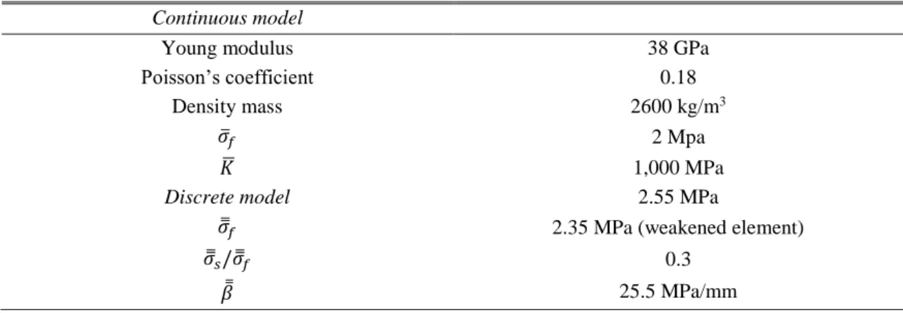
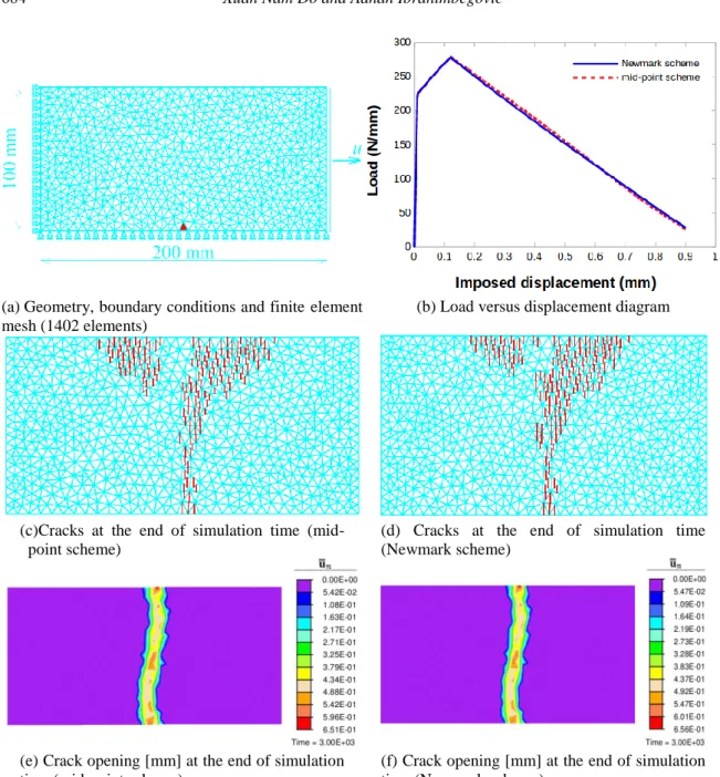
In this first example, a rectangular strip of 200 mm × 100 mm × 1 mm subjected to homogenous displacement-controlled tension applied at the right free-end is considered, see Fig. 3(a) for an illustration. It is important to note that a single element in mesh (red area) is slightly weakened to better orientate the macro-crack occurrence. Table 2 indicates the chosen values of material parameters of the specimen.
Table 2 Material properties of the specimen Continuous model
Young modulus 38 GPa
Poisson’s coefficient 0.18
Density mass 2600 kg/m3
𝜎̅𝑓 2 Mpa
𝐾̅ 1,000 MPa
Discrete model 2.55 MPa
𝜎̿𝑓 2.35 MPa (weakened element)
𝜎̿𝑠/𝜎̿𝑓 0.3
𝛽̿ 25.5 MPa/mm
According to the results in Figs. 3(c) and (d), it can be seen that for both schemes macro-cracks originate from the weakened element in mesh and then go through the center of neighboring elements in the direction perpendicular to the principal stress after the maximum principal stress reaches the chosen damage threshold value. In addition, a comparison between the results obtained with the mid-point scheme and the Newmark scheme in terms of the load versus displacement response (Fig. 3(b)) and in terms of crack opening at the end of the computation (Figs. 3(e) and (f)) also shows a small difference.
4.2 Three-point bending test
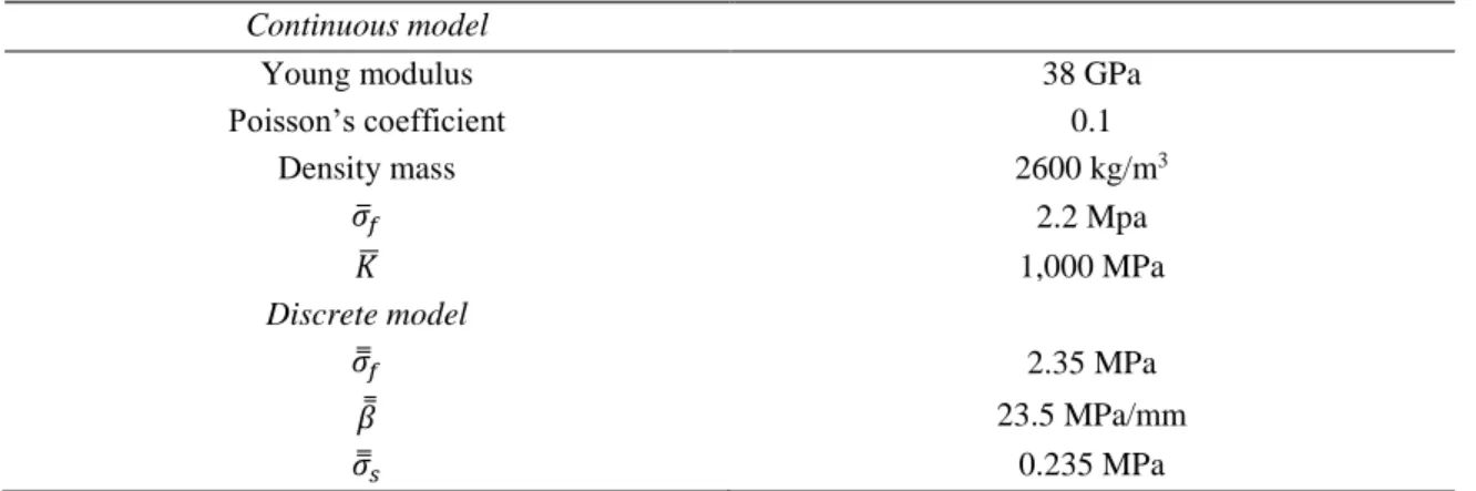
The second example presents the classical three-point bending test on a notched concrete beam (see Petersson (1981), Rots et al. (1985) and references therein). Fig. 4 describes the geometry of the specimen (a 1800 mm × 500 mm × 1mm plain concrete beam with a 20 mm × 200 mm × 1mm notch at its bottom center), the boundary conditions and the corresponding finite element mesh (1722 elements). In order to ensure this element test is performed under displacement control, the beam is simply loaded by imposed downward displacements at its center top. The set of considered material parameters is given in Table 3.
(a) Geometry, boundary conditions and finite element mesh (1402 elements)
(b) Load versus displacement diagram
(c)Cracks at the end of simulation time (mid-point scheme)
(d) Cracks at the end of simulation time (Newmark scheme)
(e) Crack opening [mm] at the end of simulation time (mid-point scheme)
(f) Crack opening [mm] at the end of simulation time (Newmark scheme)
Fig. 3 Set up for the simple tension test (a), and comparison between the mid-point scheme and the Newmark scheme (b), (c), (d), (e), (f)
Fig. 4 Three-point bending test: problem definition (a) Geometrical properties (in mm) and boundary conditions, (b) Finite element mesh (1722 elements)
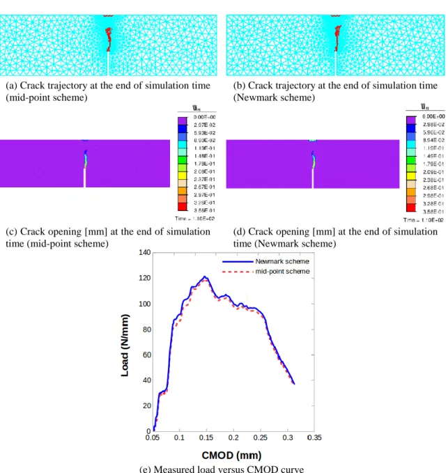
(a) Crack trajectory at the end of simulation time (mid-point scheme)
(b) Crack trajectory at the end of simulation time (Newmark scheme)
(c) Crack opening [mm] at the end of simulation time (mid-point scheme)
(d) Crack opening [mm] at the end of simulation time (Newmark scheme)
(e) Measured load versus CMOD curve
Fig. 5 Comparison between the mid-point scheme and the Newmark scheme for the three-point bending test
Results in Figs. 5(a) and (b) point out that the trajectory of development of the crack for the mid-point scheme and the Newmark scheme is fairly the same and agrees quite well with experimental results. Namely, from the experimental point of view, the crack is allowed to initiate at the notch and propagates perpendicularly to the length of the beam. Moreover, it can be observed from Figs. 5(c) and (d) that the values of crack opening computed with the mid-point scheme and the Newmark scheme are almost equivalent.
As for Fig. 5(e) in which measured load is plotted against the crack mouth opening displacement (CMOD), we find once again that the global response for both schemes above is very
Table 3 Material properties of the model in the three-point bending test Continuous model
Young modulus 38 GPa
Poisson’s coefficient 0.1 Density mass 2600 kg/m3 𝜎̅𝑓 2.2 Mpa 𝐾̅ 1,000 MPa Discrete model 𝜎̿𝑓 2.35 MPa 𝛽̿ 23.5 MPa/mm 𝜎̿𝑠 0.235 MPa
close and shows a general rule with absolute vertical or relative horizontal evolution of displacement as a function of applied loading.
Finally, it is interesting to note that for the mid-point scheme by adding viscosity parameter and by employing the time step ∆𝑡 = 2. 10−2 𝑠 which is twice as big as the time step exploited for the Newmark scheme (∆𝑡 = 10−2 𝑠) the total number of iteration is significantly reduced (23,841
versus 25,125 by the Newmark scheme) while the convergence of the solution is still ensured (in case of the Newmark scheme the solution cannot produce a good convergence with an increase to 2. 10−2 𝑠 of ∆𝑡).
4.3 Four-point bending test
We deal now with the challenging benchmark problem of a notched concrete beam under four-point bending, reported by Arrea and Ingraffea (1982) among others. The geometry of the problem is sketched in Fig. 6(a), where four blocks located between the imposed load and the concrete beam as well as between the supports and the concrete beam are steel caps with Young’s modulus
E = 288 GPa, density mass of 7830 kg/m3 and Poisson’s coefficient equal to 0.18. The finite
element mesh (1710 CST elements) is presented in Fig. 6(b). The main difference with the three-point bending test considered in Section 4.1 is that in this case the external load is applied on the steel caps at the top surface of the beam. The material properties are given in Table 4.
Fig. 6 Notched concrete specimen: (a) geometry (in mm) with L = 1322 mm, h = 306 mm, a = 14 mm, b = 82 mm and boundary conditions, (b) finite element mesh (1710 elements)
Table 4 Material properties for the four-point bending test Continuous model
Young modulus 28.8 GPa
Poisson’s coefficient 0.18 Density mass 2600 kg/m3 𝜎̅𝑓 2.6 Mpa 𝐾̅ 1,000 MPa Discrete model 𝜎̿𝑓 2.8 MPa 𝛽̿ 28 MPa/mm 𝜎̿𝑠 0.28 MPa
(a) Crack trajectory at the end of simulation time (mid-point scheme)
(b) Crack trajectory at the end of simulation time (Newmark scheme)
(c) Crack opening [mm] at the end of simulation time (mid-point scheme)
(d) Crack opening [mm] at the end of simulation time (Newmark scheme)
(e) Load-CMOD response
As can be seen from results in Figs. 7(a) and (b), the main crack in both schemes, the mid-point and Newmark, starts at the top right corner of the notch and then propagates up and to the right, the same as observed in experiment. However, different from static/quasi-static case, in the framework of dynamic loading, beside this main crack, secondary crack propagated at the position close to the external load P of the specimen since no tracking algorithm has been used to enforce only one crack. It is worth noting that the cracks are propagated by the stress concentration at the crack tip, while the failure direction is governed by the stress distribution.
Turning to the Figs. 7(c) and (d), where the main crack and the secondary crack predicted above are revealed more obviously, we can figure out that the local results in terms of crack opening remain quite similar for these two types of scheme.
Last but not least, in order to seek a good agreement between the mid-point scheme and the Newmark scheme a comparison in terms of global response is needed. More specifically, Fig. 7(e), which plots the load versus CMOD (crack mouth opening displacement) curve, shows a small gap and a quite identical trend in the path of computation of these two schemes, namely: the evolution of displacement as a function of applied loading.
5. Conclusions
In this paper, a two-dimensional continuum viscodamage-embedded discontinuity model, which combines the pre-peak nonlinear and rate-sensitive hardening response of the material behavior, representing the fracture-process zone creation and the post-peak response, involving the macro-crack creation accompanied by exponential softening, has been developed. The element tests and representative numerical simulations presented above illustrate good performance of the proposed model. Specially, by adding the viscosity parameter and by using the second-order mid-point scheme that allows bigger time steps the time for computation can be significantly reduced while the convergence is still ensured well. This feature is the main advantage of the presented scheme in comparison with the Newmark scheme and is the main novelty of this work. As a consequence, the proposed model is very suitable for long computations and high frequency problems.
Acknowledgments
Xuan Nam Do and Adnan Ibrahimbegovic would like to thank the Hauts-de-France Region (CR Picardie) (120-2015-RDISTRUCT-000010 and RDISTRUCT-000010) and the European Regional Development Fund (ERDF) 2014/2020 for Chaire-de-Mecanique (120-2015-RDISTRUCTF-000010 and RDISTRUCTI-000004) for the funding of this work. This support is gratefully acknowledged.
References
Alfaiate, J., Wells, G.N. and Sluys, L.J. (2002), “On the use of embedded discontinuity elements with crack path continuity for mode-I and mixed-mode fracture”, Eng. Fract. Mech., 69(6), 661-686.
localization in inelastic solids. In Owen, E., Onate, D.R.J., Hinton, E. (Eds)”, Proceedings of the Computational Plasticity IV, CIMNE, Barcelona, 547-561.
Armero, F. and Linder, C. (2009), “Numerical simulation of dynamic fracture using finite elements with embedded discontinuities”, Int. J. Fract., 160(2), 119-141.
Arrea, M. and Ingraffea, A.R. (1982), Mixed-Mode Crack Propagation in Mortar and Concrete, Report No. 81-13, Department of Structural Engineering, Cornell University, Ithaca, New York, U.S.A.
Bažant, Z.P. (1976), “Instability, ductility, and size effect in strain-softening concrete”, J. Eng. Mech. Div., 102, 331-344.
Bažant, Z.P., Belytschko, T.B. and Chang, T.P. (1984), “Continuum theory for strain softening”, J. Eng. Mech., 110(12), 1666-1691.
Brancherie, D. and Ibrahimbegovic, A. (2009), “Novel anisotropic continuum-discrete damage model capable of representing localized failure of massive structures. Part I: Theoretical formulation and numerical implementation”, Eng. Comput., 26(1/2), 100-127.
Cervera, M., Oliver, J. and Manzoli, O. (1995), “A rate dependent isotropic damage model for the seismic analysis of concrete dams”, Earthq. Eng. Struct. Dyn., 25, 987-1010.
De Borst, R., Sluys, L.J., Muhlhaus, H.B. and Pamin, J. (1993), “Fundamental issues in finite element analyses of localization of deformation”, Eng. Comput., 10, 99-121.
Do, X.N., Ibrahimbegovic, A. and Brancherie, D. (2017), “Dynamics framework for 2D anisotropic
continuum-discrete damage model for progressive localized failure of massive structures”, Comput.
Struct., 183, 14-26.
Dujc, J., Brank, B. and Ibrahimbegovic, A. (2013), “Stress-hybrid quadrilateral finite element with embedded strong discontinuity for failure analysis of plane stress solids”, Int. J. Numer. Meth. Eng., 94(12), 1075-1098.
Fahrenthold, E.P. (1991), “A continuum damage for facture of brittle solids under dynamic loading”, J. Appl. Mech., 58(4), 904-909.
Geuzaine, C. and Remacle, J.F. (2009), “Gmsh: A 3-d finite element mesh generator with built-in pre- and post-processing facilities”, Int. J. Numer. Meth. Eng., 79(11), 1309-1331.
Grady, D.E. and Kipp, M.E. (1980), “Continuum modelling of explosive fracture in oil shale”, Int. J. Rock Mech. Min. Sci. Geomech. Abstr., 17(3), 147-157.
Hamdi, E., Romdhane, N.B. and Le Cléac’h, J.M. (2011), “A tensile damage model for rocks: Application to blast induced damage assessment”, Comput. Geotech., 38(2), 133-141.
Huespe, A.E., Oliver, J., Sanchez, P.J., Blanco, S. and Sonzogni, V. (2006), “Strong discontinuity approach in dynamic fracture simulations”, Mecán. Comput., 25, 1997-2018.
Ibrahimbegovic, A. and Melnyk, S. (2007), “Embedded discontinuity finite element method for modeling of localized failure in heterogeneous materials with structured mesh: an alternative to extended finite element method”, Comput. Mech., 40(1), 149-155.
Ibrahimbegovic, A. and Wilson, E.L. (1991), “A modified method of incompatible modes”, Commun. Appl. Numer. Meth., 7(3), 187-194.
Linder, C. and Armero, F. (2007), “Finite element with embedded strong discontinuities for the modeling of failure in solids”, Numer. Meth. Eng., 72(12), 1391-1433.
Lu, Y. and Xu, K. (2004), “Modelling of dynamic behaviour of concrete materials under blast loading”, Int. J. Sol. Struct., 41(1), 131-143.
Needleman, A. (1988), “Material rate dependence and mesh sensitivity in localization problems”, Comput. Meth. Appl. Mech. Eng., 63(1), 69-85.
Oliver, J. (1996), “Modelling strong discontinuities in solid mechanics via strain softening constitutive equations. Part I & Part II”, Int. J. Numer. Meth. Eng., 39(21), 3575-3623.
Oliver, J. (2000), “On the discrete constitutive models induced by strong discontinuity kinematics and continuum constitutive equations”, Int. J. Sol. Struct., 37(48-50), 7207-7229.
Petersson, P.E. (1981), Crack Growth and Development of Fracture Zones in Plain Concrete and Similar Materials, Report No. TVBM-1006, Division of Building Materials, University of Lund, Lund, Sweden. Radulovic, R., Bruhns, O.T. and Mosler, J. (2011), “Effective 3D failure simulations by combining the
advantages of embedded strong discontinuity approaches and classical interface elements”, Eng. Fract. Mech., 78(12), 2470-2485.
Rots, J.G., Nauta, P., Kusters, G.M.A. and Blaauwendraad, J. (1985), “Smeared crack approach and fracture localization in concrete”, Heron, 30(1), 1-48.
Saksala, T., Brancherie, D., Harari, I. and Ibrahimbegovic, A. (2015), “Combined continuum damage-embedded discontinuity model for explicit dynamic fracture analyses of quasi-brittle materials”, Int. J. Numer. Meth. Eng., 101(3), 230-250.
Simo, J.C. and Rifai, M.S. (1990), “A class of mixed assumed strain methods and the method of incompatible modes”, Int. J. Numer. Meth. Eng., 29(8), 1595-1638.
Simo, J.C., Oliver, J. and Armero, F. (1993), “An analysis of strong discontinuity induced by strain softening solutions in rate-independent solids”, J. Comput. Mech., 12(5), 277-296.
Suaris, W. and Shah, S.P. (1984), “Rate-sensitive damage theory for brittle solids”, J. Eng. Mech., 110(6), 985-997.
Taylor, L.M., Chen, E.P. and Kuszmaul, J.S. (1986), “Microcrack-induced damage accumulation in brittle rock under dynamic loading”, Comput. Meth. Appl. Mech. Eng., 55(3), 301-320.
Wang, Z., Li, Y. and Wang, J.G. (2008), “A method for evaluating dynamic tensile damage of rock”, Eng. Fract. Mech., 75(10), 2812-2825.
Yang, R., Bawden, W.F. and Katsabanis, P.D. (1996), “A new constitutive model for blast damage”, Int. J. Rock Mech. Min. Sci. Geomech. Abstr., 33(3), 245-254.
Yazdchi, M., Valliappan, S. and Zhang, W. (1996), “Continuum model for dynamic damage evolution of anisotropic brittle materials”, Int. J. Numer. Meth. Eng., 39(9), 1555-1583.
Zienkiewicz, O.C. and Taylor, R.L. (1989), The Finite Element Method: Basic Formulation and Linear Problems, McGraw-Hill, London, U.K.