Reliability approach in spacecraft structures

To cite this document: Roussouly, Nicolas and Salaün, Michel and Petitjean,

Frank and Buffe, Fabrice and Carpine, Anne Reliability approach in spacecraft

structures. (2009) In: ECSSMMT 2009 - 11th European Conference on

Spacecraft Structures, Materials and Mechanical Testing, 15-17 Sep 2009,

Toulouse, France.

O

pen

A

rchive

T

oulouse

A

rchive

O

uverte (

OATAO

)

OATAO is an open access repository that collects the work of Toulouse researchers and

makes it freely available over the web where possible.

This is an author-deposited version published in:

http://oatao.univ-toulouse.fr/

Eprints ID: 8903

Any correspondence concerning this service should be sent to the repository

administrator:

staff-oatao@inp-toulouse.fr

RELIABILITY APPROACH IN SPACECRAFT STRUCTURE

Nicolas ROUSSOULY(1)(2)_{, Michel SALAUN}(2)_{, Frank PETITJEAN}(1)

Fabrice BUFFE (3)_{, Anne CARPINE}(4)

(1) _{Institut Catholique d’Arts et Métiers (ICAM), 75 avenue de Grande Bretagne, 31300 Toulouse, France}

nicolas.roussouly@icam.fr, frank.petitjean@icam.fr, 05.34.50.50.16

(2) _{Université de Toulouse, ISAE, 10 avenue Edouard Belin 31055 Toulouse, France}

michel.salaun@isae.fr, 05.61.33.92.83

(3)_{Centre National d’Etudes Spatiales (CNES), 18 Avenue Edouard Belin 31401 Toulouse, France}

fabrice.buffe@cnes.fr, 05.61.28.34.65

(4)_{Thales Alenia Space, 100 boulevard du Midi 06156 Cannes la Bocca, France}

anne.carpine@thalesaleniaspace.fr, 04.92.92.65.07

ABSTRACT

This paper presents an application of the probabilistic approach with reliability assessment on a spacecraft structure. The adopted strategy uses meta-modeling with first and second order polynomial functions. This method aims at minimizing computational time while giving relevant results. The first part focuses on com-putational tools employed in the strategy development. The second part presents a spacecraft application. The purpose is to highlight benefits of the probabilistic ap-proach compared with the current deterministic one. From examples of reliability assessment we show some advantages which could be found in industrial applica-tions.

INTRODUCTION

Up to now, mechanical analysis in spacecraft struc-ture has been deterministic. Numerical values of input variables are specified in order to guarantee structural performance in the worst cases. Structure validation is based on safety margin calculation which contains safety factors. This approach aims at simplifying the problem of uncertainties by makeing sure they are cov-ered but is unable to bring under control neither risk of failure nor oversizing of the structure.

For several years, certain approaches to take into ac-count uncertainties in modeling have arisen. The prob-abilistic approach is one of them and consists of consid-ering uncertainties as probabilistic ones, i.e with

ran-dom variables characterised by their probability den-sity function (pdf). This procedure gives more infor-mation like output uncertainties, reliability with re-spect to a failure mode or sensitivity of input variables. These aspects are very helpful in industrial applica-tions especially in risk analysis and in order to find an optimal design from an economical point of view that deals with technical and financial information.

To formalize the reliability concept we consider

X = {X1, ..., Xn} an input random vector with n

ran-dom variables with a joint probability density function

f_X(x) and a performance function G(X) which de-fines three mechanical domains : (a) domain of suc-cess : G(X) > 0, (b) limit state : G(X) = 0 and (c) domain of failure : G(X) < 0. Then probability of failure reads

Pf =

ˆ

G(X)<0

fX(x)dx

and reliability, called F , is equal to F = 1 − Pf. Therefore, the probability of failure calculation im-plies knowledge of the joint pdf and evaluation of the performance function. Joint pdf is generally assumed because of the lack of information on marginal laws and variable correlation. In large scale structures, per-formance function stems from a finite element code and the number of parameters to take into account grow significantly which is increasingly time consum-ing. Moreover, it is often necessary to determine re-liability with respect to several performance functions because of the number of mechanical components and

load cases.

Several method have been developed to handle these problems [8], [6]. Although simulation methods such as Monte Carlo or improved techniques are robust, they are computationally too demanding for assessing low probability of failure, i.e lower than 10−6_{. Other}

meth-ods, like first and second order reliability methmeth-ods, commonly called FORM and SORM exist. They use an optimization algorithm to find the most probable fail-ure point and then approximate the limit state (with a first or second order function) in order to assess prob-ability of failure. Such methods are interesting with a regular limit state and a low probability of failure but require an optimization procedure per response. An-other idea to achieve propagation of uncertainties is meta-modeling as an approximation of a finite element model. They are widely used in other domains of sci-ence and their efficiency in mechanical structure has al-ready been proved. The most commonly used are first and second order response surface, polynomial chaos, kriging or radial basis function but there also exists more complicated kinds of meta-models such as neural networks or support vector machines [2]. In industrial cases, advantages can be found in meta-models. They can be treated with a relatively low computational cost by comparison with a finite element one. Moreover, as a result of lack of knowledge about uncertainty of vari-ables, repeating a study with the lowest cost to assess importance of pdf is necessary. Finally, they may be useful in optimization and reliability based optimiza-tion.

In this paper we propose to use first or second order polynomial functions which are sufficiently well suited approximations in case of linear elastic behavior un-der static load with low variation on parameters. In the next section we present some computational tools used. The procedure is then applied to a spacecraft structure in order to obtain reliability results on com-ponents which can potentially fail at first. Since the finite element model is not updated after a first failure we are not able to take into account successive failures. Finally, the kind of results and benefits obtained will be discussed.

1

1.1

A finite element model of an industrial structure con-tains a lot of variables and it is often computationally too demanding to include all of them into the study.

0.0 0.2 0.4 0.6 0.8 1.0 0. 0 0.1 0 .2 0 .3 0.4 0 .5

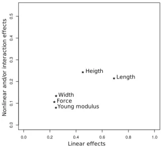
Figure 1: Graphical result of Morris OAT experiment

Generally, it appears that only a few influence studied responses. Therefore, detecting a couple of the most relevant is valuable and can be done through sensitiv-ity analysis. Some methods exist in computer simula-tion whose purpose is to rank input variables in terms of their importance. These techniques are known as screening methods and are able to deal with hundreds variables (more information on screening methods can be found in [11]). One-at-a-time (OAT) design pro-posed by Morris [9] appeared to be a good compro-mise between computational cost and the relevance of results [7]. Morris OAT is a global sensitivity exper-iment because it covers the entire space over which variables vary. It is used to distinguish (a) negligible effects, (b) linear effects without interactions, and (c) non-linear effects and/or interactions. In practice, re-sults are plotted on a graph which represents non-linear and/or interaction effects versus linear effects. Figure 1 shows an example of a Morris OAT experiment for the displacement at the end of a bending embedded beam in terms of force, young modulus, length, width and height. The number of computer runs is equal to 3(n + 1) where n is the number of variables (it could be more but 3(n + 1) is enough to obtain good infor-mation). Morris OAT doesn’t really quantify the sen-sitivity of variables but rather gives a hierarchy. More than in probabilistic approach, this kind of method can help in model understanding, optimization and model

updating. When it is used in variable selection, se-lected variables will be considered as random variables characterized by their distribution while others will be fixed to deterministic values. Therefore, meta-models will only link selected variables to studied responses. The meta-modeling process imply several steps which are presented now.

1.2

Experimental design specifies a set of input values for which finite element computation is performed in or-der to get corresponding outputs. Well known tech-niques called Design of Experiment (DOE) are gen-erally used in physical experiments. They focus on planning the experiment in order to satisfy some op-timality criteria based on physical random error. In our study, the experiment is a computer deterministic simulation and some distinctions such as random er-ror or number of factors and their range of variation can be noticed. In this way, many authors advise the use of “space filling” design in order to best cover the design space. Methods like latin hypercube sampling (LHS) or low discrepancy sequences which imply uni-form distribution of points in space are often used in literature [14, 12, 11, 10]. We will afterward perform LHS technique.

1.3

In this paper we use first and second order polyno-mial functions as an approximation of the finite ele-ment model in linear regression. The linear regression equation is given by

Y = Xβ + ε (1)

where Y is the vector of output values Yp with p ∈ [1, P ] at each sample, X is a k × p matrix where

k∈ [1, N ] which represents a matrix of regressors, β is

the vector of parameters βkwhich must be determined and ε is the vector of error εpat each sample point due to the approximation. The best way to determine pa-rameter estimation, noted ˆβ, of this model is the least square method. It appears that ˆβk depends on chosen regressors and input sample and is therefore a random variable whose quality must be guaranteed. This qual-ity is measured by the accuracy characterised by the bias (E[ ˆβk] − βk) and the stability characterized by the variance (V ar[ ˆβk]). Bias and variance are both to be minimized but are antagonists : fitting is improved when model dimension increases but the variability is

worse. Quadratic risk (QR) takes into account both aspects and is given by

QR(X ˆβ) = V ar[X ˆβ] − Bias[X ˆβ]2 (2) If we suppose that for all p, εp is an independently, normally distributed random variable of zero mean and with a variance noted σ2_{, then QR can be estimated}

by the well known Mallows Cp criteria. Other criteria exist based on other formulations than QR to check model quality. The most well-known are Akaike Infor-mation Criteria (AIC) and Bayesian InforInfor-mation Cri-teria (BIC) (see more details in [1, 5]). These criCri-teria can be used to compute the best model from several potential regressors. This is known as stepwise regres-sion. Another interesting measure used in stepwise re-gression is the R-square coefficient. It represents the fraction of variation of output explained by the model and therefore indicates how well the model reproduces output. R-square coefficient varies between 0 and 1, and is equal to 1 if the model perfectly fits the sample. Actually this coefficient increases in terms of the num-ber of regressors and is equal to 1 when the numnum-ber of regressors is equal to the number of samples. We will prefer to use the adjusted R-square, noted adjR-square, which is the R-squared penalized by the num-ber of terms [5].

Mallows Cp, AIC and BIC are based on the normal distribution of error εp in linear regression which is a classical assumption in statistics to approximate phys-ical experiments. Although in our case the experiment is deterministic and terms of error εp only specify the meta-model lack of fit, these tools can be used as a guideline but is unable to conclude about model valid-ity. The validation step is done without assumptions.

1.4

Previous criteria used in stepwise regression are more or less restrictive and result in different models. Se-lection of the best model must be done with respect to its ability to predict responses from a new input sample. The best way would be to have two samples, one for learning step and another for selection but this process imply a larger computational time. A possi-ble approach is the use of cross-validation techniques. This method consists of the following steps : (a) split the global sample into D samples, (b) leave one sam-ple out (called the validation samsam-ple) and build the model with the others, (c) use the validation sample to assess the approximation error, (d) repeat previous

steps with all samples. Then, prediction error is esti-mated as the mean of errors computed on all validation samples. The measure of error used is the classical root mean square error (RMSE). Therefore among all mod-els proposed by stepwise regression, the one with the lowest prediction RMSE is chosen.

To assess model accuracy in the region of interest we also compute the error MAX on validation samples, given by maxp∈[1,P ]( --Yp− ˆYp

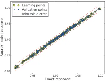
--) which estimates a more local error than RMSE. The validation of the model is guaranteed if predicted RMSE and predicted MAX are lower than a threshold. In our case, we use as the threshold 5% of maximum variation of the response. This ensures that error due to the meta-model is low with respect to response variation. From a graphical point of view, a good way to assess model accuracy is to plot response of the finite element model versus response of the meta-model with the domain of admis-sible error (cf. Figure 2).

Figure 2: Meta-model accuracy

Once the meta-model is built and validated, it is used as a surrogate of the finite element model. It is then employed in probabilistic procedures in order to anal-yse output uncertainty and to assess reliability infor-mation.

1.5

We present here the manner in which the previously described tools are used in application.

The morris OAT method is performed on the fi-nite element model but no variable selection is done. Therefore, we decided to build linear meta-models with all variables from a Latin Hypercube sampling with 3(n + 1) points which are necessary for the validation step (n is the number of variables). For each response, three linear models are established through stepwise regression with Mallows Cp, BIC and adjR-square cri-teria (Mallows Cp and AIC are equivalent in linear regression [13]). The best one is chosen from predicted RMSE computed with the cross-validation technique. If predicted MAX error and predicted RMSE are lower than admissible error (5% of maximum variation of response), the linear model is validated. If not, we add quadratic and cross-product regressors of the most significant variables selected with Morris OAT from the value indicating non-linear and/or interaction ef-fects. Since stepwise regression has removed useless linear regressors, added quadratic and cross-product terms do not involve more sampling points. This pro-cedure avoids performing more finite element compu-tation than necessary. It allows a sufficiently accurate model to be obtained in the following application. In other cases, if more regressors are useful, we must add sampling points and thus perform more finite element computation. Finally, if second order polynomial func-tions are not good enough, more sophisticated meta-models have to be used.

2

STRUCTURE

The following example involves the TARANIS space-craft whose platform belongs to the Myriade family developped by CNES. The analysis has been treated under 8 quasi-static load cases which are those of the qualification step.

2.1

The mechanical model is deterministic and has been done with the finite element code MSC NASTRAN. Figure 3 presents the finite element model. It con-tains about 380 000 degrees of freedom. Loads consist of acceleration of −9.5g in longitudinal direction (X direction) and 5.2g in lateral direction (Y and Z di-rection). Eight cases are different projection of lateral load on Y and Z axis, they are presented in Table 1. We have to notice that the model has been optimized and resultant values are not those provided by CNES.

Acceleration on axis (g) Cases X Y Z 100 -9.75 5.20 0.00 200 -9.75 3.68 3.68 300 -9.75 0.00 5.20 400 -9.75 -3.68 3.68 500 -9.75 -5.20 0.00 600 -9.75 -3.68 -3.68 700 -9.75 0.00 -5.20 800 -9.75 3.68 -3.68

Table 1: Load cases

Figure 3: TARANIS finite element model

2.2

Studied responses are maximum Von Mises stress in lateral and top panels (honeycomb with aluminium skins), in bottom panel (bulk machining aluminium) and forces in interface screws between the bottom panel and lateral panels. As the bottom panel (cf. Fig-ure 4) is more complicated than a simple plate (con-trary to other panels), maximum stress in each part such as stiffener, coupling ring, bases, etc is considered as one response. In this way, taking into account all load cases, the number of the most critical responses to study is 60 (the most critical responses are these

Figure 4: Bottom panel of TARANIS

whose deterministic safety margin is low). All input parameters of the previous components are taken as random variables (but remain constant on the sub-structure), i.e thicknesses and all material properties (Young modulus, Poisson coefficient, shear modulus, ...) which involves n = 83 variables. Random vari-ables are considered uncorrelated and distributions are assumed uniform for thicknesses (with an uncertainty of ±0.1 mm) and normal for material properties (with a coefficient of variation of 5%).

The methodology described in section 1.5 is applied on the spacecraft. Latin Hypercube sampling and Mor-ris OAT are performed on ±20% of variation on each variable. These two methods each involve 252 finite element computations (see time computation in Table 3).

2.3

Uncertainty of responses can be analysed from a Monte Carlo sampling. It gives statistical measures of re-sponse such as its expectation and standard deviation (and higher order moment) but a probability density function can also be determined thanks to a statistical hypothesis test.

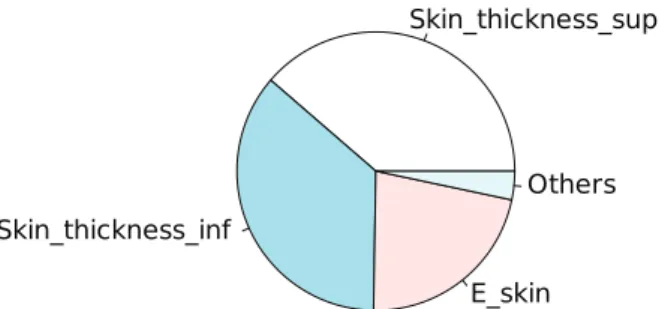
Figure 5: Variance decomposition on the +Z panel stress response

Another interesting analysis consists of variance de-composition of responses (see more details in [11]). This procedure aims at identifying the fraction of the total variance of a response which is due to any indi-vidual input variables. Figure 5 shows the variance de-composition of Von Mises stress in +Z panel (i.e panel whose normal direction is +Z).

2.4

Reliability assessment implies the definition of a per-formance function for each response. By comparison with a deterministic approach, failure modes consid-ered are the elastic limit for panels and the sliding limit for interface screws. These two limits involve new random variables (elastic limit, friction coefficient, pre-load) which are assumed independent (with a normal distribution and a coefficient of variation equal to 10%) for each component and with respect to those already defined in the finite element model. This can be a strong assumption especially between the elastic limit and the young modulus of a material which could be correlated.

As the mechanical model is a system, components depend on each others and only potential first failures can be determined. If one component fails, the finite element model does not enable to know what happen afterward and it is not able to take into account succes-sive failures. The probabilities of failure are assessed through a Monte Carlo analysis with 107_{samples (see}

time computation in Table 3).

2.4.1 Probability of failure results

Results are given in Table 2. It only contains the worst load case, i.e the case which involves the largest prob-ability of failure. For this case, components which are able to fail are presented with their probability of fail-ure and their percentage of first failfail-ure.

−0.2 0.0 0.2 0.4 0.6 0.8 0.0 0.5 1.0 1.5 2.0 2.5 3.0

Figure 6: Representation of performance function dis-tribution with reliability result on +Z panel

Case Component Probability

of failure Percentage of first failure 400 +Z panel Screw 125 Screw 112 Screw 126 Screw 113 1.9 10−3 1.87 10−5 <10−6 <10−6 <10−6 98.94 0.96 0.05 0.03 0.02 Table 2: Reliabilty results

Results show that +Z panel under case 400 is the most critical element. The probability that Von Mises stress exceeds the elastic limit of material is 1.9 10−3_.

Figure 6 shows the probability of failure of +Z panel with the distribution of performance function. For this kind of component and failure mode, such a high value could be problematic. This kind of problem would be missed in a deterministic approach since calculated safety margin is equal to 0.23. Another interesting result is the percentage of first failure which indicates how many times the component fails in a first instance. This information could be helpful in envisaging con-struction of system failure scenario.

2.4.2 Some examples of the benefits

We present here two examples which emphasize the benefits of a reliability approach compared to a deter-ministic one.

The first one is an illustration of safety margin calcula-tion versus reliability assessment. We consider here the

sliding limit of two interface screws between -Z panel and -X panel under load case 700. We assume that the friction coefficient and pre-load follow a normal distri-bution with 0.23 and 17260N respectively for the mean and 10% for both coefficient of variation [4]. In a de-terministic approach, the safety margin is calculated with a B-value for friction coefficient and with a value lower than a B-value for pre-load (all other variables are considered at their mean). Moreover a safety co-efficient of 1.25 is considered. From this configuration the sliding margin is negative and is equal to −0.022 for one screw and −0.017 for the other. This can create some problems in a qualification step. With a reliabil-ity approach random variables are considered, charac-terized by the previous distributions. Moreover, the safety coefficient is removed. In this case, probabilities that screws slide are 7.2 10−4_{and 6.5 10}−4_{respectively.}

This kind of probability of failure could be considered as acceptable in this context.

The second example illustrates the importance of re-liability assessment in order to compare two manufac-turing processes of aluminium panel skins. Skin thick-nesses are assumed to follow a uniform distribution with a mean of 0.6 mm. With such a low thickness, two manufacturing processes are considered, one ex-pensive with good accuracy which implies a thickness variation of ±5% ; one cheaper with a lower accuracy which implies a thickness variation of ±20%. Prob-abilities that Von Mises stresses exceed elastic resis-tances (under case 400) are 1.9 10−3_{and 3.47 10}−4

re-spectively. Considering manufacturing costs of both processes, a well-founded decision can be taken which deals with the technical risk and financial aspect [3].

CONCLUSION

This paper presents two main issues. On one hand, we attempted to show the relevance of results which arise from a probabistic approach and more precisely in reli-ability assessment. Although current deterministic ap-proach is firmly fixed in structural analysis, it doesn’t enable to improve designs with respect to robustness or reliability linked with economical constraints whihc are always more and more restrictive. A probabilistic approach is one of possible means and is starting to be applied in several industrial domains. Of course, cur-rent practices will not be replaced but it is a way to enrich them with more accurate information especially in order to help in decision. Making this kind of

ap-Step Time

Morris OAT 9h30

Latin Hypercube Sampling 9h30 Meta-models construction 20 min 107 _{samples on meta-models 1h}

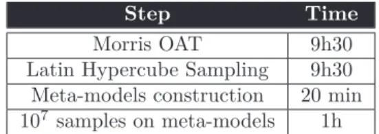
Table 3: Time computation of each step in methodol-ogy. Desktop computer used is a dual core 2.8 GHz, 1.97 Go RAM

proach can bring benefits to the definition of less con-servative sizing rules. On the other hand, we presented a resolution strategy based on meta-modeling. It can be employed on quite large structures and is not too computationally time demanding. Table 3 resumes the computational time of each step of methodology. Even if it could appear large relatively to a deterministic ap-proach, it is very fast when compared with a direct Monte Carlo on finite element model which would last 43 years. Finally advantages of meta-models are nu-merous. Structural behaviour can be represented well even with simple models : linear polynomial functions are often sufficient. Although in our case the structure is linear elastic under quasi-static load with low varia-tions, more sophisticated meta-models could deal with more complicated mechanical behaviour. Meta-models are also re-usable in order to measure the influence of stochastic chosen input parameters. This seems to be an essential point as distribution of random variables are usually assumed because of the lack of databases. Another interest of meta-models can be found in opti-mization or more precisely reliability based optimiza-tion.

References

[1] J. Azaïs and J. Bardet. Le modèle linéaire par l’exemple. Tech. rep., Université Paul Sabatier. [2] R. R. Barton. Metamodeling : a state of the art

review. In Proceedings of the 1994 Winter

Simu-lation Conference. 1994.

[3] J. Buffe. Aide à la prise de décision, gestion des risques. Tech. rep., Thales Alenia Space, 2006. [4] A. Carpine. Faisabilité d’un dimensionnement

basé sur une approche stochastique. Tech. rep., Thales Alenia Space, 2009.

[5] P. Cornillon and E. Matzner-Lober. Régression,

[6] O. Ditlevsen and H. Madsen. Structural reliabil-ity methods. Tech. rep., Section of Coastal, Mar-itime and Structural Engineering, Department of Mechanical Engineering, 2007.

[7] B. Garnier. Etude des méthodes d’analyse de

sen-sibilité, application aux structures spatiales.

Mas-ter’s thesis, ENSMA, 2009.

[8] M. Lemaire. Fiabilité des structures. Hermes, 2005.

[9] M. D. Morris. Factorial sampling plans for prelim-inary computational experiments. Technometrics, 33:161–174, 1991.

[10] J. Sacks, W. Welch, et al. Design and analysis of computer experiments. Statistical science, pp. 409–423, 1989.

[11] A. Saltelli, K. Chan, et al. Sensitivity analysis.

Series in Probability and Statistics. Wiley, 2000.

[12] T. Simpson, J. Poplinski, et al. Metamodels for Computer-based Engineering Design: Survey and recommendations. Engineering with Computers, 17(2):129–150, 2001.

[13] M. Stone. An asymptotic equivalence of choice of model by cross-validation and Akaike’s criterion.

Journal of the Royal Statistical Society. Series B (Methodological), pp. 44–47, 1977.

[14] G. Wang and S. Shan. Review of Metamod-eling Techniques in Support of Engineering De-sign Optimization. Journal of Mechanical DeDe-sign, 129:370, 2007.