Pépite | Analyse qualitative de plusieurs types de systèmes de maladies infectieuses avec effets de réaction ou de diffusion

Texte intégral

(1)Thèse de Mengfeng Sun, Université de Lille, 2019. N◦ d’ordre : 108414. THÈSE présentée à L’UNIVERSITÉ DE LILLE en cotutelle avec l’Université de Shanghai, Chine pour obtenir le titre de DOCTEUR DE L’UNIVERSITÉ Spécialité : Mathématiques par. Mengfeng SUN. Analyse qualitative de plusieurs types de systèmes de maladies infectieuses avec effets de réaction ou de diffusion Soutenue le 6 juin 2019 devant le jury composé de :. Présidente : Dongmei XIAO, Shanghai Jiaotong University, China Rapporteurs : Yuan YUAN, Memorial University of Newfoundland, Canada Directeurs : Guoting CHEN, Université de Lille, France Xinchu FU, Shanghai University, China Examinateurs : Luonan CHEN, Tokyo University, Japan Mei SUN, Jiangsu University, China Rapporteur absent à la soutenance : Vincent NAUDOT, Florida Atlantic University, USA. Thèse préparée au sein de École Doctorale Sciences Pour l’Ingénieur. © 2019 Tous droits réservés.. Laboratoire Paul Painlevé. lilliad.univ-lille.fr.

(2) Thèse de Mengfeng Sun, Université de Lille, 2019. © 2019 Tous droits réservés.. lilliad.univ-lille.fr.

(3) Thèse de Mengfeng Sun, Université de Lille, 2019. Acknowledgements The successful completion of my Ph.D. program is inseparable from many people. I would like to express my gratitude for each of them right now. First and foremost, I would like to thank my supervisor, Prof. Guoting Chen, for his guidance on the course of my doctoral degree and academic research. When I was at Lille University (France), he tried his best to provide me with a good research environment. Despite his busy schedule, he always took the time to provide unique insights into my work and mathematical problems. I would also like to express my heartfelt thanks to my supervisor at Shanghai University (China), Prof. Xinchu Fu. Thanks for his guidance, help, encouragement and persistent support at all stages of the Ph.D. program. In the past few years, he has been continuously discovering my potential, so that I can do the best I can. His supervision and inspiration are invaluable, and it is my honor to cooperate with him. I want to thank the two “rapporteurs de ma thèse”, Prof. Vincent Naudot at Florida Atlantic University and Prof. Yuan Yuan at Memorial University of Newfoundland, for taking their valuable time to read my manuscript carefully, as well as their insightful comments and helpful suggestions for revision, having made this thesis a better work. I thank the president of my thesis defense committee: Prof. Dongmei Xiao at Shanghai Jiaotong University, and members of the committee: Prof. Luonan Chen at Tokyo University and Chinese Academy of Sciences and Prof. Mei Sun at Jiangsu University, for taking time out of their busy schedule to attend my doctoral thesis defense. I am especially grateful to thank Prof. Michael Small at the University of Western Australia, who is my main collaborator with Prof. Yijun Lou at the Hong Kong Polytechnic University and the driving force behind our work. Thanks to my other close collaborators, Prof. Jinqiao Duan at the Illinois Institute of Technology and Prof. Shui Shan Lee at the Chinese University of Hong Kong, who have been very enthusiastic about our joint efforts. Thanks for their interesting discussions, positive advice, and fruitful cooperation. I am very happy to have the opportunity to work with each of them. I would like to thank the members of the Biomathematics Research Group for their valuable and constructive discussions. In particular, I am very grateful to Prof. Ping Ao, Prof. Xinjian Xu, Prof. Ruiqi Wang and Prof. Jie Lou for giving me a lot of help, as well as comments on my research ideas and methods. Many thanks to the School of Mathematics at Lille University and the Department of Mathematics at Shanghai University for providing me with rich resources and places. Special thanks to secretaries Aurore Smets, Yilian Fan and Danqing Cao, and the librarian, for their support and assistance during my Ph.D.. Furthermore, I gratefully acknowledge the financial support from the program of China Scholarships Council (Grant No. 201606890057), which allowed me to continue my doctoral study. Many friends, colleagues and groups have become part of my life in Lille and Shanghai. Thanks to senior fellow apprentices: Haifeng Zhang, Guanghu Zhu, Yizhou Tao, Kezan Li and Zhaoyan Wu; senior sister apprentices: Huiyan Kang, Lingna Wang and Shanshan Chen; and junior sister apprentice Yumei Cui, for all their assistance and advice in scientific research and life. Meanwhile, I also thank my classmate Zhongpu Xu, junior fellow apprentice: Junbo Jia, Pan Yang, Yu Wang and Wei Shi, for their enthusiasm and encouragement in the past few years. I am also very grateful to the colleagues of System Biology Lab: Yanwei Liu, Yanfen. © 2019 Tous droits réservés.. lilliad.univ-lille.fr.

(4) Thèse de Mengfeng Sun, Université de Lille, 2019. ii. Dai, Yujing Luo. With them, I spent a lot of good time, leaving a wonderful memorable moment. In addition, I would like to thank my roommate Gang Qiao, my friends: Min Wang, Haowu Wang, Lian Yang, Wenjie Chen, Yin Xu, Yanni Xu, etc, for their support all the time. Last but not least, I am deeply indebted to my family. Thank my parents for their endless love and “time-invariant” support for me. Whenever I talk to them about something, whether it is important or not, they are willing to listen. Their encouragement helped me and was the motivation and foundation of my study. Also, my sister and brother-in-law, thanks for their care and understanding during the long doctoral period. I am very grateful to have such a happy family, so that my doctoral studies can be satisfactorily and smoothly completed.. © 2019 Tous droits réservés.. lilliad.univ-lille.fr.

(5) Thèse de Mengfeng Sun, Université de Lille, 2019. Contents Chapter 1. Introduction 1. Background and objectives 2. Main work of the thesis. 1 1 7. Chapter 2.. Traveling waves and estimation of minimal wave speed for a diffusive influenza system with multiple strains 1. Preliminary lemma on the existence of equilibria for the reaction system 2. Semi-traveling waves for an auxiliary system 2.1. An auxiliary system 2.2. Linearization of the wave system at E 0 2.3. Construction and properties of upper-lower solutions 2.4. The existence of semi-traveling waves 3. Semi-, strong and weak traveling waves for the original system 3.1. Semi-traveling waves 3.2. Strong traveling waves 3.3. Weak traveling waves 4. Nonexistence of semi-traveling waves and estimation of minimal wave speed for the original system 4.1. Nonexistence of semi-traveling waves 4.1.1. Case I: RC < 1 and c > 0 4.1.2. Case II: RRC > 1, RSC ̸= 1 and 0 < c < c∗1 4.1.3. Case III: RSC > 1, RRC ̸= 1 and 0 < c < c∗2 4.1.4. Case IV: RC > 1, Ri ̸= 1, i = SC, RC and 0 < c < min{c∗1 , c∗2 } 4.2. Estimation of the minimal wave speed 5. Concluding remarks Dynamical behavior for a class of predator-prey type eco-epidemiological systems in R3+ 1. Conley index and restricted Conley index 1.1. Conley index 1.2. The restricted Conley index 2. Preliminary lemmas 3. Dynamics of three subsystems 3.1. S-I subsystem 3.2. S-P subsystem 3.2.1. Local stability of boundary equilibria 3.2.2. Main results with monotonic functional response. 11 13 15 16 16 18 21 25 25 28 32 36 36 36 37 40 41 41 42. Chapter 3.. 43 43 43 45 46 49 51 57 58 59. i. © 2019 Tous droits réservés.. lilliad.univ-lille.fr.

(6) Thèse de Mengfeng Sun, Université de Lille, 2019. ii. 0 Contents. 3.2.3. Main results with non-monotonic functional response 3.3. I-P subsystem 4. Dynamical analysis of the full system 4.1. Boundary equilibria and their stability 4.2. Uniform persistence 4.3. Robustness of heteroclinic orbits and a heteroclinic network 4.4. An interior periodic orbit 5. Concluding remarks. 61 64 65 66 69 70 71 73. Chapter 4.. Mathematical analysis of network-based systems coupling epidemic spread and information diffusion 75 1. Complex networks and network-based approaches for epidemic spread 75 2. A concrete interplay system and its stability analysis 76 2.1. A concrete interplay system 76 2.2. Stability analysis 79 2.2.1. Preliminaries 79 2.2.2. Epidemic threshold 80 2.2.3. Global stability 82 3. Epidemic control system and its stability analysis 87 3.1. Epidemic control system 87 3.2. Stability analysis 87 4. Numerical simulations 89 5. Concluding remarks 92. References. © 2019 Tous droits réservés.. 93. lilliad.univ-lille.fr.

(7) Thèse de Mengfeng Sun, Université de Lille, 2019. CHAPTER 1. Introduction 1. Background and objectives The research of infectious diseases based on mathematical models, especially dynamic models, has a long and diverse history [40]. It may be traced back to D. Bernoulli’s mathematical study of smallpox vaccination in 1760 [15]. In 1873-1894, P. D. En’ko established modern mathematical models of infectious diseases [36]. In 1906, in order to understand the repeated epidemics of measles, W. H. Hamer constructed a discrete mathematical model and analyzed the dynamics of the model [49]. Five years later, the Nobel laureate, R. Ross, used a differential dynamical system to study the dynamics of malaria transmission between mosquitoes and people in detail [94]. To study the epidemic regularity of black death in 1665-1666 and plague in 1906, W. O. Kermack and A. G. McKendrick proposed the most influential model—SIR model in 1927 [5, 59]:  dS   = −βSI,     dt dI (1.1) = βSI − γI,  dt      dR = γI, dt where the total population (N ) in the affected area is divided into three classes: susceptible (S), infected (I) and recovered (R). Birth and death are ignored, that is, N (t) = S(t) + I(t) + R(t) is constant. The parameters β and γ denote the transmission and recovery rates, respectively. Subsequently, W. O. Kermack and A. G. McKendrick put forward the SIS compartmental model in 1932 [60]:  dS   = −βSI + γI, dt (1.2)   dI = βSI − γI. dt On this basis, they proposed a “threshold theory” that distinguishes whether the disease 0 becomes popular. When the basic reproduction number R0 := βS γ < 1, the disease dies out; when R0 > 1, the disease remains and becomes endemic, where S0 denotes the number or density of the initial susceptible population. These two basic dynamic models (SIR and SIS) and the corresponding theories established by W. O. Kermack and A. G. McKendrick lay a foundation for the study of the dynamics of infectious diseases. Since then, mathematical modeling and dynamical analysis of infectious diseases began to flourish, and the representative work is the first book on the mathematical theory of infectious diseases and its applications published by N. T. Bailey in 1957 [9]. Especially in the past 30 years, there has been a rapid progress for the mathematical analysis of the dynamical systems originating from infectious diseases in the world. A large number 1. © 2019 Tous droits réservés.. lilliad.univ-lille.fr.

(8) Thèse de Mengfeng Sun, Université de Lille, 2019. 2. 1 Introduction. of papers and books [5, 50, 58] have been devoted to analyze the dynamical properties of the established models with regard to various infectious diseases. In this thesis, we shall consider three types of dynamical systems extracted from infectious disease research, i.e., (a) reaction-diffusion system, (b) ordinary differential system, and (c) network-based system. The first two categories are deterministic models, and the last one belongs to stochastic models. Systems (a) and (c) have the diffusion effect, while system (b) only has the reaction effect. In what follows, we introduce their research progress in recent years, respectively. (I) A diffusive influenza system with multiple strains Influenza, having been a major cause of excessive morbidity and mortality [102], is a serious cytopathogenic, drastic respiratory infectious disease caused by an RNA virus in the Orthomyxoviridae family [35]. Besides, influenza poses a considerable economic burden of society and becomes a problem of public health [113]. Thus, it is imperative to prevent and contain the outbreak of influenza via increasing our understanding of the dynamics of influenza transmission. Among pharmaceutical interventions, antiviral treatment remains one of the most effective measures to lower disease transmission and reduce the health burden of infections [38]. On the other hand, abundant use of antiviral drugs (such as oseltamivir and zanamivir) is a significant factor in producing resistant strains. Recently, some mathematical models have been used to explore the potential effects of drug resistance on the transmission of influenza [93] and identify effective treatment strategies for resistance management [69, 91]. These studies have provided useful insights into the emergence, spread and control of drugresistant influenza. However, these models are all ordinary differential models. If the random movement of individuals in space plays a very important role in the dynamics of influenza transmission, it is necessary to consider the influence of spatial diffusion, which is usually characterized by reaction-diffusion equations. The traveling wave solution (or referred to as traveling wave), which appears to be traveling with constant shape and velocity, is one of the elementary notions in the study of reaction-diffusion equations. The study of traveling wave solutions for nonlinear reactiondiffusion equations began with Fisher’s equation. In 1937, R. A. Fisher proposed the following equation [39]: ut = d∆u + ru(1 − u), t > 0, x ∈ Rn , (1.3) ∑n ∂ 2 where ∆ = i=1 ∂x2 , the parameters r and d are both positive, to describe the spatial spread i of an advantageous allele and explored its traveling wave solutions. At the same time, A. N. Kolmogorov et al. gave a more general reaction-diffusion equation [61]: ut = duxx + f (u), t > 0, x ∈ R,. (1.4). and analyzed its traveling wave solutions. Thereafter, traveling wave solutions of nonlinear reaction-diffusion equations have been extensively and deeply studied, wherein its existence is the most fundamental problem in determining the long-term behavior of other solutions of the systems [54, 96, 122]. In epidemiology, the existence and nonexistence of nontrivial traveling waves indicate whether an infectious disease can persist as a wave front of infection that travels geographically across vast distances. The minimal wave speed for a traveling wave is a key parameter to characterize the speed at which the disease spreads in a spatial. © 2019 Tous droits réservés.. lilliad.univ-lille.fr.

(9) Thèse de Mengfeng Sun, Université de Lille, 2019. 1. BACKGROUND AND OBJECTIVES. 3. domain [33, 96]. Therefore, the study of traveling waves and minimal wave speeds is of great significance to the prevention and control of diseases. In 2014, T. Zhang and W. Wang established a reaction-diffusion influenza model with treatment [123]:   ∂S ∂2S   = d − β(Iu + δIh )S, s   ∂x2  ∂t    ∂ 2 Iu ∂Iu   = du 2 + (1 − µ)β(Iu + δIh )S − ku Iu , ∂t ∂x (1.5)  ∂ 2 Ih ∂Ih   = dh 2 + µβ(Iu + δIh )S − kh Ih ,   ∂x  ∂t   2R  ∂ ∂R   = dr 2 + ku Iu + kh Ih , ∂t ∂x and focused on the existence and nonexistence of traveling wave solutions. As a result of the high mobility of population and the emergence of drug resistance due to treatment, we will further show the effects of demographic factors (recruitment and natural deaths) and drug resistance on the spatial spread of influenza. With the increase of the practical factors, some interesting and novel dynamics will appear, which are different from those in previous studies [122, 123, 124]. (II) Predator-prey type eco-epidemiological systems Ecology [76] and epidemiology [5], as two different subjects in the field of mathematical biology [79], have received considerable attention in their own right. However, since R. M. Anderson and R. M. May (1978, 1986) showed that invasion of a resident predator-prey (or host-parasite) system by a new strain of parasites could cause destabilization and give rise to limit cycles [4, 77], quite a number of research papers (e.g., see [6, 25, 47, 72, 109] and the references in [72]) have already appeared in this intercrossed direction, linking ecological and epidemiological issues together. This leads to a new field of research popularly known as eco-epidemiology, which is coined by J. Chattopadhyay and O. Arino [25]. In studying eco-epidemiological systems, the interaction between species are primarily assumed to be predator-prey type [4, 6, 25, 47, 72, 77], although competitive type [4, 72] and symbiotic type [72, 109] are also common. In terms of predator-prey type eco-epidemiological systems, disease spread can happen within prey/host population [4, 6, 25, 72, 77], or within predator/host population [4, 72], or between prey and predator populations [47]. From the perspective of modeling, the dynamical behavior of predator-prey system with infection in the prey population is an important research topic. Generally speaking, such eco-epidemiological system with SI or SIS type disease (see [4, 6, 25, 72, 77]) can be defined by the following Kolmogorov-type differential equations  dS   = Sf1 (S, I, P ),     dt dI (1.6) = If2 (S, I, P ),  dt      dP = P f3 (S, I, P ), dt in the state space R3+ = {(S, I, P ) ∈ R3 : S ≥ 0, I ≥ 0, P ≥ 0},. © 2019 Tous droits réservés.. lilliad.univ-lille.fr.

(10) Thèse de Mengfeng Sun, Université de Lille, 2019. 4. 1 Introduction. where S(t), I(t) and P (t) represent the population densities/numbers of susceptible prey, infected prey, and predator at time t, respectively. The functions fk ∈ C 1 (R3+ , R), k = 1, 2, 3. Since eco-epidemiological system (1.6) is a combination of a predator-prey model and an epidemiological model, there are two factors that need attention from a large perspective: (i) the choice of predator-prey model, generalized Gause or Leslie-Gower type [72]; (ii) the types of infectious diseases, SI or SIS [5, 79]. On the other hand, Allee effect is an important dynamic phenomenon in conservation biology, which is named after W. C. Allee(1885-1955) [32]. In recent decades, researchers have conducted extensive theoretical studies on Allee effect within different biological contexts, such as biological invasion [110], infectious diseases [51], etc. However, to the best of our knowledge, there is little research involving the impact of Allee effect on eco-epidemiology [17, 56, 97], wherein [17, 56] considered the case that susceptible prey is subject to Allee effect. Given the above considerations, system (1.6) can be simplified to a less abstract but biologically more intuitive system as follows:  dS   = Sg(S, I)a(S, θ) − ψ(S, I) − ϕ1 (S, I, P )P,     dt dI (1.7) = ψ(S, I) − ϕ2 (S, I, P )P − µI,  dt      dP = γ1 ϕ1 (S, I, P )P + γ2 ϕ2 (S, I, P )P − dP, dt where the parameters d and µ represent the death rate (includes an additional disease-induced death) of the predator and infected prey, γ1 and γ2 are the conversion rates of the susceptible and infected prey biomass into the predator biomass, respectively; g(S, I) denotes the per capita growth rate of susceptible prey in the absence of Allee effect and predation; a(S, θ) models an Allee effect that affects susceptible prey; ψ(S, I) is the transmission/incidence function; ϕ1 (S, I, P ) and ϕ2 (S, I, P ) are the functional/trophic responses or feeding rates for the predator with respect to susceptible and infected preys, respectively. In particular, we assume that infected prey has less but positive contribution to the growth of the predator in comparison to susceptible prey, that is, 0 < γ2 < γ1 . Moreover, µ, d, γ1 and γ2 lie in the interval (0, 1). The form of carrying capacity plays a central rule in the function g(S, I), which usually has two types, namely, explicit and implicit/emergent carrying capacities [99]. In most of the model-based eco-epidemiological studies [6, 17, 25, 47, 56, 97], especially when resources are limited, the growth function with explicit carrying capacity (wherein the competitive abilities for both susceptible and infected preys are the same) is a better choice as it is easy to interpret and comparatively straightforward to estimate from real life observations. However, the experimental study in [13] suggests that disease can change the competitive abilities within prey. For this reason, we first assume that infected prey does not contribute to the reproduction of newborns but competes for resources. By considering different competition coefficients for two possible interactions, based on the growth function c1 S+c2 I g(S, I) = rS(1− S+I ), K ) with explicit carrying capacity, we modify it as g(S, I) = rS(1− K where c1 and c2 (0 < c1 , c2 ≤ 1) represent the weights of intra-class competition in susceptible prey and inter-class competition between susceptible and infected preys, respectively. Although the mathematical expressions modeling Allee effect are varied [31, 108], most of them can be proven to be topologically equivalent. Here, we adopt the most common form for Allee effect [62], i.e., a(S, θ) = S − θ, where − cK1 ≤ θ ≪ cK1 . When θ > 0, this phenomenon. © 2019 Tous droits réservés.. lilliad.univ-lille.fr.

(11) Thèse de Mengfeng Sun, Université de Lille, 2019. 1. BACKGROUND AND OBJECTIVES. 5. is called a strong Allee effect [108, 110], and θ is known as Allee threshold. When θ ≤ 0, it is said that susceptible prey is affected by a weak Allee effect [110]. The transmission/incidence function is usually either density-dependent (also referred to the law of mass action or the bilinear incidence, i.e., ψ(S, I) = kSI) or frequency-dependent kSI (also called the standard incidence, i.e., ψ(S, I) = S+I ) [20]. By taking into account more biological details, several different nonlinear transmission functions (e.g., the saturated transβSI mission rate 1+αI [23] and nonlinear incidence βS p I q [70]) were proposed. We think the saturated transmission form is more reasonable since it represents a “crowding effect” or “protection measure” and prevents the unboundedness of the contact rate, so in our work, βIS 1 we use ψ(S, I) = 1+αI , where α > 0, βI measures the infection force of the disease and 1+αI measures the inhibition effect from the behavioral change of susceptible prey when their number increases or from the crowding effect of infective prey. Different functional responses have been considered in the context of ecology and ecoepidemiology, see [10, 21, 80]. Mathematically, they can be classified into two main categories: monotonic and non-monotonic. To keep systems more general, the functional response is not specified in our work. Moreover, we assume that the predator is not smart enough to distinguish between susceptible and infected preys. Hence, the algebraic expresbS m sions of ϕk (S, I, P ), k = 1, 2 used in this work take ϕ1 (S, I, P ) = (S+I) n +an and ϕ2 (S, I, P ) = bI m (S+I)n +an ,. where n, m ∈ N+ , n ≥ m ≥ 1, b is the searching efficiency constant or the predation rate on the prey and a is the half-saturation constant of the predator. Our model (1.7) is different from the models used in the previous works [17, 56, 97] due to several aspects: (D1) We use different competition coefficients within prey that arises due to disease-modified inter-specific competition. This is an extension of the initial idea of M. Sieber et al. [99]. (D2) The incidence function exhibits the feature of transmission saturation. (D3) The predator not only captures infected prey but also catches susceptible prey based on the work of S. Biswas et al. [17]. Moreover, the consumption of infected prey has less contribution to the predator’s growth. (D4) We use the generalized functional responses of the predator, whose advantage is that our results are not restricted to a particular model but applicable to certain classes of models. (III) Network-based systems coupling epidemic spread and information diffusion Complex networks have recently attracted attention in many disciplines, including epidemiology, physics, and social sciences [57]. Whereas the conventional compartmental models of epidemic transmission are based on the assumption of a homogenous and well-mixed population, the application of complex networks explicitly models connectivity between individuals. In particular, the discovery of scale-free networks has shifted the focus of network-based research on disease transmission from small world networks to scale-free networks [11]. One of the most influential results is the pioneering work done by R. Pastor-Satorras and A. Vespignani [86, 87, 88]. After that, more and more scholars concentrate on the study of epidemic models on complex networks [19, 81, 85]. In real-world situations, when an epidemic begins to spread, people generally become increasingly aware of its presence. Their perception of the nature of the epidemic is shaped by the information obtained through a variety of distinct channels: in their social or spatial neighborhood, from the mass media (e.g., TV, radio, newspapers, etc.), through various. © 2019 Tous droits réservés.. lilliad.univ-lille.fr.

(12) Thèse de Mengfeng Sun, Université de Lille, 2019. 6. 1 Introduction. online social media, and under the influence of various environmental factors. This spreading information then causes some people to change their behaviors — either to protect themselves or to reduce the risk of transmission [37]. As a result, the extent of the spread of the infection can be significantly reduced [43]. This implies that the outbreak of an epidemic can trigger behavioral responses from individuals, conversely, human behavioral changes induced by epidemics could have great influence on the epidemic dynamics and even epidemic network structure. So, it is of great interest to incorporate the change of human behaviors into mathematical models for infectious disease transmission, making an exploration and simulation of epidemic spread and its control. Recently, several works have addressed the problem from different perspectives [8, 42, 64, 74, 116], for example, risk perception, behavioral changes, competing viral agents, or collective behaviors. For simplicity, we collectively denote all individual and community preventive behaviors against epidemics as adaptive behaviors. To examine the interplay between adaptive behaviors and epidemic spread, in Fig. 1, we depict a specific logical loop in the process of epidemic spread. Therefore, in order to accurately model the spread of epidemics in complex Aw areness. B ehavi or i nformati on transmi ssi on. Epi demi c i nformati on. Adapti ve behavi ors. Epi demi c. Figure 1. A specific logical loop in the process of epidemic spread. networks, we should take account of multiple dynamic processes simultaneously, including epidemic spread, behavioral dynamics, information transmission, and the interplay. A general interplay model between human adaptive behaviors and epidemic spread in complex networks can be described by  ˙  X(t) = F (X(t), C(t)), (1.8) Y˙ (t) = G(Y (t), E(t)),  ˙ C(t) = H(Y (t), E(t)), where the variable X(t) = (xT1 (t), xT2 (t), · · · , xTN (t))T with xi (t) = (xi1 (t), xi2 (t), · · · , xin (t))T ∈ Rn denotes the behavior state variable of all individuals in a behavior information network with size N , which can display collective behaviors under suitable conditions. The variable C(t) = (c1 (t), c2 (t), · · · , cN (t))T with ci (t) ∈ R denotes the coupling weight of each individual in the behavior information network. In the second equality of (1.8), the variable Y (t) = (y1 (t), y2 (t), · · · , yN (t))T with yi (t) ∈ R denotes the infection probability of each individual in an epidemic spreading network with size N . The variable E(t) = (E1 (t), E2 (t), · · · , EN (t))T with Ei (t) ∈ R denotes the state error of each individual, which can be defined in different forms. F, G, and H represent three different mappings, respectively. The mapping F : (RnN , RN ) → RnN controls the dynamical change process of the state variable X(t). The mapping G : (RN , RN ) → RN characterizes the dynamical change process of the infection probability Y (t). The mapping H : (RN , RN ) → RN defines an adaptive update law of the coupling weight C(t).. © 2019 Tous droits réservés.. lilliad.univ-lille.fr.

(13) Thèse de Mengfeng Sun, Université de Lille, 2019. 2. MAIN WORK OF THE THESIS. 7. In system (1.8), human adaptive behaviors X(t) play a role in the epidemic spreading process Y (t) by embedding the behavior state error E(t), and epidemic spreading process Y (t) influences human adaptive behaviors X(t) by changing their coupling weight C(t). Knowing that the spread of behavioral information is quite different from that of the underlying epidemic, we intend to study the complex interplay between adaptive behaviors and epidemic spread in multiplex networks [103], in which the nodes represent the same entities in all layers but the connection patterns at each layer are different. In view of the authenticity of the network and the accuracy of feedback of nodes (i.e., point-to-point feedback), the topological structure of a multiplex network is set to be quenched. On the other hand, for emerging epidemics, people cannot promptly manufacture effective vaccines or produce targeted drugs. In these circumstances, governments, mass media, or public health authorities typically choose to guide individual behaviors to an optimal state of self-protection to reduce one’s susceptibility to infection, so we will design optimized control schemes from the new perspective of behavioral regulation. From a mathematical point of view, we shall focus on the qualitative structure (or topological structure) of the limit sets (or invariant sets) in these three classes of dynamical systems. The limit sets usually contain at least one of the following three parts: (1) singularities/equilibria, (2) periodic solutions (closed orbits), and (3) singularities and the orbits which tend to these singularities when t → −∞ or t → +∞ (e.g., homoclinic and heteroclinic orbits). Supposing that the limit sets of systems are discussed clearly, their qualitative structure can be basically determined. Furthermore, the stability of the limit sets and bifurcation phenomena are also the main content of our concern. 2. Main work of the thesis This thesis is divided into five chapters, and mainly studies the dynamical behavior of three types of epidemiological mathematical systems, i.e., a diffusive influenza system with multiple strains, predator-prey type eco-epidemiological systems, and two network-based systems coupling epidemic spread and information diffusion. For these epidemiological systems, we focus on their qualitative analysis. The specific work of this thesis is stated as follows. In Chapter 2, we consider the following diffusive influenza system with multiple strains  ∂S ∂2S    = dS 2 + Λ − µS − [βS (ISU + δIST ) + βR IR ]S,   ∂t ∂x     ∂ 2 ISU ∂ISU   = d + (1 − f )βS (ISU + δIST )S − (kU + µ)ISU , SU   ∂x2   ∂t ∂IST ∂ 2 IST (1.9) + f (1 − r)βS (ISU + δIST )S − (kT + µ)IST , = d ST 2  ∂t ∂x     ∂IR ∂ 2 IR   = d + [f rβS (ISU + δIST ) + βR IR ]S − (kR + µ)IR , R   ∂t ∂x2    2  ∂R ∂ R   = dRe 2 + kU ISU + kT IST + kR IR − µR. ∂t ∂x Our main purpose is to establish the conditions for the existence of the three kinds of traveling waves for system (1.9) starting from the disease-free equilibrium E 0 (S 0 , 0, 0, 0, 0) (at the initial stage of influenza transmission): semi-traveling waves, strong traveling waves and weak (persistent) traveling waves.. © 2019 Tous droits réservés.. lilliad.univ-lille.fr.

(14) Thèse de Mengfeng Sun, Université de Lille, 2019. 8. 1 Introduction. So far, the existence of traveling waves for monotone systems (e.g., competitive or cooperative models) has been well understood. However, system (1.9) is a non-monotone system, implying that some standard methods, such as the monotone iteration and comparison argument [68, 126], are no longer suitable. Though there have been some recent progress in the study of non-monotonic systems [2, 54, 120, 122, 123, 124], the methods in these references (such as singular perturbation argument, geometric method, squeeze method, etc.) seem to be powerless for system (1.9). Several specific reasons are: (i) The non-monotonic systems in the above literatures mostly consist of two equations, while system (1.9) contains five equations; (ii) Unlike the handling techniques in [123], we have no restrictions on the diffusion coefficients of different variables; (iii) To be more realistic, recruitment and natural mortality factors of population are considered, which increase the dynamical complexity of the system. Due to the complexity of system (1.9), some dynamical problems on this system become very challenging, implying that we need to improve the previous approaches. To do so, we shall further extend the method of upper-lower solutions developed in [2, 122, 123, 124]. Since it is difficult to construct a pair of appropriate upper-lower solutions connecting the diseasefree equilibrium E 0 for system (1.9), we first introduce an auxiliary system, the existence of semi-traveling waves of which is easy to prove. The existence of semi-traveling waves of the auxiliary system, together with limit arguments imply the existence of semi-traveling waves of system (1.9). Then we construct an appropriate Lyapunov function and apply persistent theory of dynamical systems in [105] to prove the existence of strong and weak traveling waves of system (1.9), respectively. Finally, the nonexistence of semi-traveling waves for system (1.9) in four cases is obtained by the comparison principle, the negative one-sided and two-sided Laplace transforms, which are introduced by [24, 124]. Furthermore, the interval estimation of the minimal wave speed is given. In Chapter 3, we study a class of predator-prey type eco-epidemiological systems in R3+ , given by the following set of nonlinear differential equations:  c1 S + c2 I βI bS m dS   = rS(1 − )(S − θ) − S − P,   dt K 1 + αI (S + I)n + an   dI m βI bI = S− P − µI, (1.10)  dt 1 + αI (S + I)n + an  m m  dP  bS bI   = γ1 P + γ2 P − dP, n n dt (S + I) + a (S + I)n + an with initial conditions S(0) ≥ 0, I(0) ≥ 0, P (0) ≥ 0.. (1.11). Our main objective is to explore the abundant dynamic behavior exhibited by the proposed system and to identify the crucial parameters that ensure specific population behaviors. Firstly, to gain insight into the boundary dynamics of system (1.10), we divide it into three independent subsystems in R2+ , that is, the epidemiological (S-I subsystem), predator-prey (S-P subsystem) and predator-infected-prey(I-P subsystem) subsystems. Then, by: (i) obtaining a global topological sketches of the dynamics of (1.10) and its three subsystems, with different Allee effects or competitive coefficients; and (ii) comparing the dynamics of (1.10) and its S-P subsystem with monotonic functional response to those with non-monotonic functional response, we conclude that (a) strong Allee effect can create a separatrix curve (or surface), leading to multi-stability; (b) different competitive abilities between prey can greatly change. © 2019 Tous droits réservés.. lilliad.univ-lille.fr.

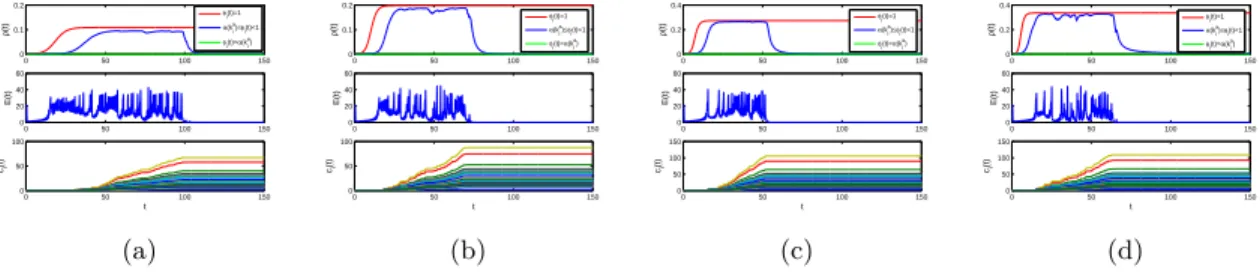
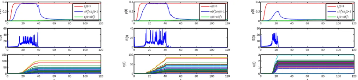
(15) Thèse de Mengfeng Sun, Université de Lille, 2019. 2. MAIN WORK OF THE THESIS. 9. the dynamics of S-I subsystem, and (c) S-P subsystem with non-monotonic functional response has richer dynamical behavior than that with monotonic functional response. Finally, we provide the sufficient conditions for the local and global stability of boundary equilibria of (1.10), derive the criteria for which (1.10) will persist, and identify an interior periodic orbit by applying Poincaré map and bifurcation theory. In Chapter 4, we present two network-based systems coupling epidemic spread and information diffusion, namely, a concrete interplay system in quenched multiplex networks  N ∑    bij Γ[xj (t) − xi (t)], x˙ i (t) = f (xi (t)) + ci (t)    j=1 N ∑ (1.12) ρ˙ i (t) = −ρi (t) + λϕi (t)[1 − ρi (t)] aij ρj (t), i = 1, 2, · · · , N,    j=1    c˙i (t) = βψ(kia )[θ(kia )ρli (t) + (1 − θ(kia ))ρg (t)]eTi (t)ei (t), and an epidemic control system  N ∑   x ˙ (t) = f (x (t)) − c (t) lij Γxj (t) + ui (t),  i i i   j=1      ui (t) = −ci (t)di ei (t), i = 1, 2, · · · , l, ui (t) = 0, i = l + 1, l + 2, · · · , N,   N ∑    ρ ˙ (t) = −ρ (t) + λϕ (t)[1 − ρ (t)] aij ρj (t), i = 1, 2, · · · , N, i i i i    j=1   c˙i (t) = βψ(kia )[θ(kia )ρli (t) + (1 − θ(kia ))ρg (t)]eTi (t)ei (t).. (1.13). Our main aim is to investigate the uniform persistence and stability of systems (1.12) and (1.13). Through the next-generation matrix approach, we calculate the basic reproduction number of the epidemic spreading system in (1.12) and (1.13), which is a critical quantity that determines whether epidemics are persistent. With the aid of the theories of nonnegative matrices, we explore the impact of adaptive behaviors on epidemic spread by comparing the epidemic thresholds. Then we utilize the comparison principle, construct appropriate Lyapunov functions and applying the LaSalle’s invariance principle to prove the globally asymptotically stability of two network-based systems, including the disease-free and endemic equilibria of the network-based epidemic spreading system and the synchronization manifold of the network-based behavioral information diffusion system. For theoretically unprovable parts, we perform some numerical simulations to supplement the mathematical analysis of systems (1.12) and (1.13).. © 2019 Tous droits réservés.. lilliad.univ-lille.fr.

(16) Thèse de Mengfeng Sun, Université de Lille, 2019. © 2019 Tous droits réservés.. lilliad.univ-lille.fr.

(17) Thèse de Mengfeng Sun, Université de Lille, 2019. CHAPTER 2. Traveling waves and estimation of minimal wave speed for a diffusive influenza system with multiple strains In this chapter, we consider the following diffusive influenza system with multiple strains  ∂2S ∂S    = dS 2 + Λ − µS − [βS (ISU + δIST ) + βR IR ]S,   ∂t ∂x     ∂ISU ∂ 2 ISU   = d + (1 − f )βS (ISU + δIST )S − (kU + µ)ISU , SU   ∂x2   ∂t ∂IST ∂ 2 IST = d + f (1 − r)βS (ISU + δIST )S − (kT + µ)IST , ST  ∂t ∂x2     ∂IR ∂ 2 IR   = d + [f rβS (ISU + δIST ) + βR IR ]S − (kR + µ)IR , R   ∂x2  ∂t    ∂R ∂2R   = dRe 2 + kU ISU + kT IST + kR IR − µR, ∂t ∂x. (2.1). where S(x, t), ISU (x, t), IST (x, t), IR (x, t) and R(x, t) represent the quantities of susceptible, infected with the sensitive strain and untreated, infected with the sensitive strain and treated, infected with the resistant strain, and recovered population at position x and time t, respectively. The parameters dS , dSU , dST , dR and dRe are the diffusion coefficients of the above five subclasses. The constant Λ is the recruitment rate of the population and µ is per-capita natural death rate. Here we assume that each infected individual with the sensitive strain will receive treatment with proportion f , and each individual who received treatment will develop drug resistance with probability r. The parameters βS and βR are the transmission coefficients of the untreated and drug-resistant infected individuals. Due to antiviral treatment, the transmission rate by an individual who received treatment will be reduced by the factor δ. Each individual in Ij subclasses can recover with the corresponding rate kj , j = SU, ST, R. All parameters are assumed to be positive. The corresponding reaction system of (2.1) is described by the following system of ODEs:  dS  = Λ − µS − [βS (ISU + δIST ) + βR IR ]S,    dt    dISU   = (1 − f )βS (ISU + δIST )S − (kU + µ)ISU ,     dt dIST = f (1 − r)βS (ISU + δIST )S − (kT + µ)IST ,  dt    dIR   = [f rβS (ISU + δIST ) + βR IR ]S − (kR + µ)IR ,    dt     dR = k I + k I + k I − µR. U SU T ST R R dt. (2.2). 11. © 2019 Tous droits réservés.. lilliad.univ-lille.fr.

(18) Thèse de Mengfeng Sun, Université de Lille, 2019. 12. 2 Traveling waves and estimation of minimal wave speed. In Section 1, we shall give conditions for the existence of equilibria of system (2.2). Under some conditions, (2.2) has a unique disease-free equilibrium E 0 , and under some other condiˆ and/or tions, apart from the disease-free equilibrium, there exist a boundary equilibrium E ∗ an interior equilibrium E . Since the first four equations of (2.1) are independent of the last one, it suffices to consider the following reduced reaction-diffusion system:   ∂S ∂2S   = d + Λ − µS − [βS (ISU + δIST ) + βR IR ]S, S   ∂t ∂x2     ∂ 2 ISU ∂ISU   = dSU + (1 − f )βS (ISU + δIST )S − (kU + µ)ISU , ∂t ∂x2 (2.3) 2  ∂IST ∂ IST   = dST + f (1 − r)βS (ISU + δIST )S − (kT + µ)IST ,   ∂t ∂x2    2   ∂IR = d ∂ IR + [f rβ (I + δI ) + β I ]S − (k + µ)I .  R S SU ST R R R R ∂t ∂x2 More specifically, we consider a solution of (2.3), (S(x, t), ISU (x, t), IST (x, t), IR (x, t)), with the following form S(x, t) = S(ξ), Ii (x, t) = Ii (ξ), ξ = x + ct,. (2.4). where i = SU, ST, R, and c > 0 is the wave speed. The solution (S(x, t), ISU (x, t), IST (x, t), IR (x, t)) having the form (2.4) is called a traveling wave solution (or referred to as traveling wave) if S(ξ) and Ii (ξ), i = SU, ST, R, are defined for all ξ ∈ R and are nonnegative functions. For the convenience of discussions below, we first list several definitions of different kinds of traveling waves as follows [2, 54, 124]. Definition 0.1. (see [2, 54]). A traveling wave (S(ξ), ISU (ξ), IST (ξ), IR (ξ)) is called a semi-traveling wave connected to the disease-free equilibrium E 0 (for convenience, here we still use the same notation E 0 to represent the equilibrium of system (2.3)) if it satisfies the boundary condition lim (S(ξ), ISU (ξ), IST (ξ), IR (ξ)) = E 0 (S 0 , 0, 0, 0).. ξ→−∞. (2.5). Definition 0.2. (see [124]). A traveling wave (S(ξ), ISU (ξ), IST (ξ), IR (ξ)) is strong if it satisfies (S(−∞), ISU (−∞), IST (−∞), IR (−∞)) = E 0 , ˆ ∗, (S(+∞), ISU (+∞), IST (+∞), IR (+∞)) = E/E. (2.6). where U (±∞) = limξ→±∞ U (ξ). Definition 0.3. (see [124]). A traveling wave (S(ξ), ISU (ξ), IST (ξ), IR (ξ)) is weak or persistent if there exist two positive constants M1 and M2 such that (S(−∞), ISU (−∞), IST (−∞), IR (−∞)) = E 0 , M1 < lim inf S(ξ), lim sup S(ξ) < M2 , ξ→+∞. ξ→+∞. M1 < lim inf Ii (ξ), lim sup Ii (ξ) < M2 , i = SU, ST, R. ξ→+∞. © 2019 Tous droits réservés.. (2.7). ξ→+∞. lilliad.univ-lille.fr.

(19) Thèse de Mengfeng Sun, Université de Lille, 2019. 1. PRELIMINARY LEMMA ON THE EXISTENCE OF EQUILIBRIA FOR THE REACTION SYSTEM. 13. The remaining parts of this chapter are organized as follows. A preliminary lemma on the existence of equilibria for the reaction system is given in Section 1. Section 2 is devoted to establish the existence of semi-traveling waves of an auxiliary system. By using the results derived in Section 2, conditions for the existence of three different kinds of traveling waves of the original system are obtained in Section 3. By means of the comparison principle and the negative one-sided and two-sided Laplace transforms, some sufficient conditions for the nonexistence of semi-traveling waves of the original system and an estimation of the minimal wave speed are given in Section 4. Finally, Section 5 concludes this work. 1. Preliminary lemma on the existence of equilibria for the reaction system In this section, we give a brief discussion about the existence of equilibria of corresponding reaction equations (2.2) of (2.1). Denote by N (t) the total quantity of the population at time t, namely, N (t) = S(t) + ISU (t) + IST (t) + IR (t) + R(t). Note that the total population quantity N (t) satisfies the equation dN = Λ − µN. (2.8) dt It is clear that N (t) = Λ µ is a solution of equation (2.8), and for any initial value N (t0 ) ≥ 0, the general solution of (2.8) is 1 N (t) = [Λ − (Λ − µN (t0 )) exp−µ(t−t0 ) ]. (2.9) µ By the expression (2.9) of the general solution of (2.8), we have limt→+∞ N (t) = Λ µ. Through the above analysis, we know that the biologically feasible set of reaction system (2.2) is given by Γ = {(S, ISU , IST , IR , R)|0 ≤ S, ISU , IST , IR , R, S + ISU + IST + IR + R ≤. Λ }. µ. (2.10). Obviously, the set Γ is positively invariant for system (2.2). There is a key parameter in epidemiological models, the basic reproduction number, commonly denoted by R0 , defined as the expected number of secondary infections generated by a single infectious individual during the infection period in an entirely susceptible population [5, 50, 119]. When certain control measures (such as immunization, isolation, treatment, etc) are introduced, we use the control reproduction number, denoted by RC , to determine whether the epidemic can be contained [5]. Similarly, we can use the same approach developed in [106] to calculate the control reproduction number of reaction system (2.2) with treatment terms. Note that system (2.2) always has a disease-free equilibrium E 0 = (S 0 , 0, 0, 0, 0), where S 0 := Λ µ . System (2.2) has three infected variables, namely, ISU , IST and IR , linearizing the equations of these three variables at disease-free equilibrium E 0 (S 0 , 0, 0, 0, 0), the matrices F and V (corresponding to the new infection and remaining transfer terms, respectively) are given by   (1 − f )βS S 0 (1 − f )βS δS 0 0 F =  f (1 − r)βS S 0 f (1 − r)βS δS 0 (2.11) 0 , 0 0 f rβS S f rβS δS βR S 0. © 2019 Tous droits réservés.. lilliad.univ-lille.fr.

(20) Thèse de Mengfeng Sun, Université de Lille, 2019. 14. 2 Traveling waves and estimation of minimal wave speed. and.  kU + µ 0 0 . V = 0 kT + µ 0 0 0 kR + µ . Thus, FV where. (. F11 =. (1−f )βS S 0 kU +µ f (1−r)βS S 0 kU +µ. −1. (1−f )βS δS 0 kT +µ f (1−r)βS δS 0 kT +µ. ( =. F11 0 F21 F22. ). ( , F21 =. (2.12). ) ,. f rβS S 0 kU +µ. f rβS δS 0 kT +µ. ) , F22 =. βR S 0 . kR + µ. Let RSU =. βS δ βR βS , RST = , RR = , kU + µ kT + µ kR + µ. (2.13). then we have RSC = ρ(F11 ) =. (1 − f )βS S 0 f (1 − r)βS δS 0 + = S 0 [(1 − f )RSU + f (1 − r)RST ], kU + µ kT + µ. (2.14). and RRC = ρ(F22 ) =. βR S 0 = S 0 RR , kR + µ. (2.15). where ρ(A) is the spectral radius of the nonnegative matrix A. Thus, the control reproduction number of system (2.2) is given by RC = ρ(F V −1 ) = max{RSC , RRC }.. (2.16). To study equilibria of system (2.2) and their corresponding conditions of parameters, we present the following lemma. Lemma 1.1. (1) The disease-free equilibrium E 0 always exists; (2) If RC < 1, there exists a unique disease-free equilibrium E 0 ; (3) If RC > 1, then in addition to the disease-free equilibrium E 0 , system (2.2) has a boundary ˆ when RRC > 1, and an interior (positive) equilibrium E ∗ when RSC > 1 and equilibrium E RRC < RSC . Proof: The equilibria of system (2.2) are the solutions of the following equations:   Λ − µS − [βS (ISU + δIST ) + βR IR ]S = 0,     (1 − f )βS (ISU + δIST )S − (kU + µ)ISU = 0,  (2.17) f (1 − r)βS (ISU + δIST )S − (kT + µ)IST = 0,    [f rβ (I + δI ) + β I ] S − (k + µ)I = 0, S SU ST R R R R    k I + k I + k I − µR = 0. U SU T ST R R In order to solve algebraic equations (2.17), we divide it into the following three cases. Case I: IR = 0. For this case, based on the setting of parameters and the fact that S > 0, from the fourth equation of (2.17), we have ISU = IST = 0. Substituting IR = ISU = IST = 0 0 into the first equation of (2.17), we can obtain S = Λ µ =S .. © 2019 Tous droits réservés.. lilliad.univ-lille.fr.

(21) Thèse de Mengfeng Sun, Université de Lille, 2019. 2. SEMI-TRAVELING WAVES FOR AN AUXILIARY SYSTEM. 15. Case II: IR > 0 and IST = 0. For this case, it follows from the third and fourth equations 0 +µ ˆ Substituting ISU = IST = 0 and S = Sˆ of (2.17) that ISU = 0 and S = kRβR = RSRC := S. into (2.17), we get the following reduced equations { Λ − µSˆ − βR IR Sˆ = 0, (2.18) kR IR − µR = 0. µS 0 (1−. 1. k S 0 (1−. ). 1. ). R RRC RRC ˆ := IˆR and R = := R. By solving (2.18), we obtain IR = kR +µ kR +µ Case III: IR > 0 and IST > 0. For this case, we first deal with the second and third equations of (2.17), which can be regarded as equations with unknown quantities ISU and IST . In view of the fact that IST > 0, by Cramer’s Rule, we have

(22)

(23)

(24) (1 − f )βS S − (kU + µ)

(25) (1 − f )βS δS

(26)

(27) = 0.

(28) f (1 − r)βS S f (1 − r)βS δS − (kT + µ)

(29). Calculate the above determinant, we can get the value of S as follows S=. (kU + µ)(kT + µ) S0 = := S ∗ . (kT + µ)(1 − f )βS + (kU + µ)f (1 − r)βS δ RSC. Substituting S = S ∗ into (2.17), after some algebraic computations, we can solve the remaining four unknown quantities of equations (2.17) with S = S ∗ as follows µ(RSC − 1) ∗ ∗ ∗ := ISU , IST = aISU := IST , βS (1 + δa) + βR b ∗ + k I∗ + k I∗ kU ISU T ST R R ∗ ∗ IR = bISU := IR , R= := R∗ , µ. ISU =. where a =. f (1−r)(kU +µ) (1−f )(kT +µ). and b =. f r(kU +µ) . R (1−f )(kR +µ)(1− RRC ) SC. From the above discussions, it follows that (2.17) has three possible nonnegative solutions. ˆ = (S, ˆ 0, 0, IˆR , R) ˆ Accordingly, system (2.2) has three possible equilibria E 0 = (S 0 , 0, 0, 0, 0), E ∗ , I ∗ , I ∗ , R∗ ). Based on the expression of Iˆ in Case II, we know that and E ∗ = (S ∗ , ISU R ST R ∗ > 0, from the expression of I ∗ in IˆR > 0 if and only if RRC > 1. Under the condition ISU R ∗ > 0 if and only if R Case III, we can easily see that IR RC < RSC , which implies b > 0. Return ∗ , we can similarly determine that I ∗ > 0 if and only if R to the expression of ISU SC > 1. SU ∗ ˆ When RC < 1, i.e., RSC < 1 and RRC < 1, it follows that IR < 0 and ISU < 0. Thus, when RC < 1, system (2.2) has a unique disease-free equilibrium E 0 . When RRC > 1, it ˆ exists. When RRC < RSC and RSC > 1, the interior follows that the boundary equilibrium E ∗ (positive) equilibrium E exists. No matter how RSC and RRC are valued, the disease-free equilibrium E 0 always exists. □ In Table 1, we present a diagram to clearly show the relationship between the existence of equilibria and the values of the parameters RSC , RRC and RC . 2. Semi-traveling waves for an auxiliary system In this section, to prove the existence of semi-traveling waves for the original system (2.3) (here, in view of the equivalence between systems (2.1) and (2.3), we also refer to system (2.3) as the original system in the latter study), we first introduce an auxiliary system, the technique of which has been widely used (see [71, 122, 123, 124]). Then, by linearizing the wave equations of the original system (2.3) at disease-free equilibrium E 0 , we construct a pair of. © 2019 Tous droits réservés.. lilliad.univ-lille.fr.

(30) Thèse de Mengfeng Sun, Université de Lille, 2019. 16. 2 Traveling waves and estimation of minimal wave speed. Table 1. Existence of equilibria on the values of RSC , RRC and RC Equilibria Parameters RC < 1 RSC > 1 > RRC RSC > RRC > 1 RRC > 1 > RSC RRC > RSC > 1. E0. ˆ E. E∗. Y Y Y Y Y. N N Y Y Y. N Y Y N N. Remark: Y: Exists; N: Does not exist. upper-lower solutions for the auxiliary system. Finally, we use Schauder’s fixed-point theorem to establish the existence of semi-traveling waves for the auxiliary system. 2.1. An auxiliary system. An auxiliary system related to the original system (2.3) can be described by  ∂S 2 = dS ∂∂xS2 + Λ − µS − [βS (ISU + δIST ) + βR IR ]S,  ∂t   ∂ISU  ∂ 2 ISU 2 ∂t = dSU ∂x2 + (1 − f )βS (ISU + δIST )S − (kU + µ)ISU − ΥISU , (2.19) 2I ∂ ∂I 2 , ST ST  = d + f (1 − r)β (I + δI )S − (k + µ)I − ΥI ST S SU ST T ST 2  ST ∂x   ∂I∂tR ∂ 2 IR 2 ∂t = dR ∂x2 + [f rβS (ISU + δIST ) + βR IR ]S − (kR + µ)IR − ΥIR , where Υ is a small positive constant. Substituting the wave profile S(x, t) = S(ξ), Ii (x, t) = Ii (ξ), i = SU, ST, R, ξ = x + ct into (2.19), and denoting x + ct by ξ, we obtain the corresponding wave equations  cS ′ = dS S ′′ + Λ − µS − [βS (ISU + δIST ) + βR IR ]S,    ′ ′′ + (1 − f )β (I 2 cISU = dSU ISU S SU + δIST )S − (kU + µ)ISU − ΥISU , (2.20) 2 ′′ + f (1 − r)β (I ′  cIST = dST IST S SU + δIST )S − (kT + µ)IST − ΥIST ,   ′ ′′ + [f rβ (I 2 cIR = dR IR S SU + δIST ) + βR IR ]S − (kR + µ)IR − ΥIR . The limiting equations of (2.20) when Υ → 0 become the wave equations of the original system (2.3). For the convenience of use, we give their specific form as follows:  cS ′ = dS S ′′ + Λ − µS − [βS (ISU + δIST ) + βR IR ]S,    ′ ′′ + (1 − f )β (I cISU = dSU ISU S SU + δIST )S − (kU + µ)ISU , (2.21) ′ ′′   cIST = dST IST + f (1 − r)βS (ISU + δIST )S − (kT + µ)IST ,  ′ = d I ′′ + [f rβ (I cIR R R S SU + δIST ) + βR IR ]S − (kR + µ)IR . 2.2. Linearization of the wave system at E 0 . Linearizing system (2.21) at the disease-free equilibrium E 0 (S 0 , 0, 0, 0) and only considering the last three equations of the linearized system, we have  ′ ′′ 0  cφ2 = dSU φ2 + (1 − f )βS (φ2 + δφ3 )S − (kU + µ)φ2 , ′ ′′ (2.22) cφ3 = dST φ3 + f (1 − r)βS (φ2 + δφ3 )S 0 − (kT + µ)φ3 ,  ′ ′′ 0 cφ4 = dR φ4 + [f rβS (φ2 + δφ3 ) + βR φ4 ]S − (kR + µ)φ4 , where the functions φi (ξ), i = 2, 3, 4 correspond to Ij (ξ), j = SU, ST, R, respectively.. © 2019 Tous droits réservés.. lilliad.univ-lille.fr.

(31) Thèse de Mengfeng Sun, Université de Lille, 2019. 2. SEMI-TRAVELING WAVES FOR AN AUXILIARY SYSTEM. 17. We look for the solutions with the form (φ2 (ξ), φ3 (ξ), φ4 (ξ)) = eλξ (κ2 , κ3 , κ4 ), where κi > 0, i = 2, 3, 4 and λ > 0. Substituting them into equations (2.22), we obtain the following eigenvalue equations  2 0  cλκ2 = dSU λ κ2 + (1 − f )βS (κ2 + δκ3 )S − (kU + µ)κ2 , 2 (2.23) cλκ3 = dST λ κ3 + f (1 − r)βS (κ2 + δκ3 )S 0 − (kT + µ)κ3 ,  2 0 cλκ4 = dR λ κ4 + [f rβS (κ2 + δκ3 ) + βR κ4 ]S − (kR + µ)κ4 . ˜ = diag(c, c, c) and M f(λ, c) := Aλ ˜ 2 − Bλ ˜ + F − V , where Let A˜ = diag(dSU , dST , dR ), B the matrices F and V are given by (2.11) and (2.12). Then the eigenvalue equations (2.23) can be rewritten as f(λ, c)K = 0, M (2.24) where K = (κ2 , κ3 , κ4 )T . ˜ we obtain the equivalent form Make the new transformation A = V −1 A˜ and B = V −1 B, of equation (2.24) as follows M (λ, c)K = K, (−Aλ2. (2.25). I)−1 (V −1 F ).. where M (λ, c) = + Bλ + A direct calculation gives   M (λ, c) =  . (1−f )βS S 0 Θ2 (λ,c) f (1−r)βS S 0 Θ3 (λ,c) f rβS S 0 Θ4 (λ,c). (1−f )βS δS 0 Θ2 (λ,c) f (1−r)βS δS 0 Θ3 (λ,c) f rβS δS 0 Θ4 (λ,c). 0 0 βR S 0 Θ4 (λ,c).   , . (2.26). where Θ2 (λ, c) = −dSU λ2 + cλ + kU + µ, Θ3 (λ, c) = −dST λ2 + cλ + kT + µ, Θ4 (λ, c) = −dR λ2 + cλ + kR + µ. c , c) is strictly increasing and nonnegative in Take d = max{dSU , dST , dR }, since Θi ( 2d c c ∈ [0, +∞), we can deduce that the matrix M ( 2d , c) is decreasing for c ∈ [0, +∞). Denote by ρ(M (λ, c)) the principal eigenvalue of the nonnegative matrix M (λ, c) for c λ ∈ [0, 2d ]. Since ρ(M (λ, c)) is continuous and monotonically increasing with respect to the c nonnegative matrix M (λ, c), ρ(M ( 2d , c)) is strictly decreasing in c ∈ [0, +∞). In particular, c −1 , c)) → 0 when c → +∞. we have ρ(M (0, 0)) = ρ(V F ) when c = 0 and ρ(M ( 2d For the continuation of the analysis, here, we give a brief proof of ρ(V −1 F ) = RC . By the definition of the control reproduction number RC in (2.16), we know RC = ρ(F V −1 ), implying that RC is the Perron-Frobenius eigenvalue of the matrix F V −1 . So there exists a positive eigenvector P = (p1 , p2 , p3 ) with pi > 0, i = 1, 2, 3 such that (F V −1 )P = RC P . Then we have V −1 P > 0 and (V −1 F )(V −1 P ) = V −1 (F V −1 )P = RC V −1 P . This implies that RC is a nonnegative eigenvalue of the matrix V −1 F with positive eigenvector V −1 P . It is easy to see that V −1 F is irreducible, that is, (V −1 F + I)2 > 0. Using Perron-Frobennius theorem, we get ρ(V −1 F ) = RC . Combining with ρ(M (0, 0)) = ρ(V −1 F ) yields ρ(M (0, 0)) = RC . Consequently, when RC > 1, there exists a unique c∗ > 0 such that  ∗  > 1, c ∈ [0, c ); c ρ(M ( , c)) = 1, c = c∗ ;  2d < 1, c ∈ (c∗ , +∞).. © 2019 Tous droits réservés.. lilliad.univ-lille.fr.

(32) Thèse de Mengfeng Sun, Université de Lille, 2019. 18. 2 Traveling waves and estimation of minimal wave speed. c Now we fix c > c∗ , note that Θi (λ, c)(i = 2, 3, 4) is strictly increasing in λ ∈ [0, 2d ], then c we obtain that ρ(M (λ, c)) is strictly decreasing and nonnegative in λ ∈ [0, 2d ]. In view of the c c facts ρ(M (0, c)) = ρ(M (0, 0)) = RC > 1 and ρ(M ( 2d , c)) < 1, then there exists a λc ∈ (0, 2d ) such that   > 1, λ ∈ [0, λc ); ρ(M (λ, c)) = 1, λ = λc ;  c < 1, λ ∈ (λc , 2d ]. Based on the above discussion, we have the following lemma.. Lemma 2.1. Assume that RC = ρ(F V −1 ) > 1. Then there exists c∗ > 0 such that for c ) and Kc = (κ2 , κ3 , κ4 )T with κi > 0, i = 2, 3, 4 any c > c∗ , we can always find λc ∈ (0, 2d f(λc , c) = 0 and M f(λc , c)Kc = 0. satisfying det M Proof: It follows from the above arguments that ρ(M (λc , c)) = 1. By the PerronFrobenius theorem, we conclude that there is a vector Kc ∈ R3 with positive components such that M (λc , c)Kc = Kc . Multiplying the matrix −Aλ2c + Bλc + I on both sides of the above equality, we have (Aλ2c − Bλc + V −1 F − I)Kc = 0. Multiplying the diagonal matrix V ˜ 2c − Bλ ˜ c + F − V )Kc = M f(λc , c)Kc = 0. □ to both sides of the above equality, we obtain (Aλ Let Kc = (κ2 , κ3 , κ4 )T as obtained in Lemma 2.1, the following lemma is straightforward. Lemma 2.2. The vector valued function φ(ξ) = (φ2 (ξ), φ3 (ξ), φ4 (ξ)) with φi (ξ) = κi eλc ξ , i = 2, 3, 4 satisfies equations (2.22). 2.3. Construction and properties of upper-lower solutions. In the next subsection, by using the Schauder’s fixed-point theorem, we establish the existence of semi-traveling waves of the auxiliary system (2.20). For this, we need to define a pair of upper-lower solutions of system (2.20) as follows. ¯ S(ξ) := S 0 , S(ξ) := max{S 0 − σeαξ , 0}, I¯SU (ξ) := min{κ2 eλc ξ , κ2 K ∗ }, I SU (ξ) := max{κ2 eλc ξ (1 − Qeεξ ), 0}, (2.27) I¯ST (ξ) := min{κ3 eλc ξ , κ3 K ∗ }, I ST (ξ) := max{κ3 eλc ξ (1 − Qeεξ ), 0}, I¯R (ξ) := min{κ4 eλc ξ , κ4 K ∗ }, I R (ξ) := max{κ4 eλc ξ (1 − Qeεξ ), 0}, where the constants κ2 , κ3 , κ4 and λc have been determined in Lemma 2.1. The positive constants K ∗ , σ, α, Q, ε will be determined later. We next show that such constructed upper and lower solutions satisfy some properties in Lemmas 2.3, 2.4 and 2.5. Lemma 2.3. For K ∗ > 1 large enough, the functions I¯SU (ξ), I¯ST (ξ) and I¯R (ξ) satisfy the following inequalities  ′ ′′ 0 2  cI¯SU ≥ dSU I¯SU + (1 − f )βS (I¯SU + δ I¯ST )S − (kU + µ)I¯SU − ΥI¯SU , ′′ + f (1 − r)β (I¯ 0 ¯ ¯ ¯2 (2.28) cI¯′ ≥ dST I¯ST S SU + δ IST )S − (kT + µ)IST − ΥIST ,  ¯ST ′ ′′ 0 cI ≥ dR I¯ + [f rβS (I¯SU + δ I¯ST ) + βR I¯R ]S − (kR + µ)I¯R − ΥI¯2 , R. for any ξ ̸= ξ1 :=. R. R. ln K ∗ λc .. Proof: Define the operator .  ′′ ′ dSU ISU − cISU + (1 − f )βS (ISU + δIST )S 0 − (kU + µ)ISU ′′ ′ L[ISU (·), IST (·), IR (·)](ξ) :=  dST IST − cIST + f (1 − r)βS (ISU + δIST )S 0 − (kT + µ)IST  , ′′ ′ dR IR − cIR + [f rβS (ISU + δIST ) + βR IR ]S 0 − (kR + µ)IR. © 2019 Tous droits réservés.. lilliad.univ-lille.fr.

(33) Thèse de Mengfeng Sun, Université de Lille, 2019. 2. SEMI-TRAVELING WAVES FOR AN AUXILIARY SYSTEM. 19. then, the differential inequalities (2.28) can be transformed into the following equivalent operator inequalities 2 2 2 L[ISU (·), IST (·), IR (·)](ξ) ≤ Υ(I¯SU , I¯ST , I¯R ).. (2.29). So, as long as we prove operator inequality (2.29), we complete the proof of the lemma. Below, we can prove operator inequalities (2.29) in two cases: When ξ < ξ1 , by (2.27), we have (I¯SU (ξ), I¯ST (ξ), I¯R (ξ)) = (κ2 , κ3 , κ4 )eλc ξ . Substituting it into the equations of operator L, yields f(λc , c)Kc = 0. L[ISU (·), IST (·), IR (·)](ξ) = eλc M Obviously, operator inequalities (2.29) hold. When ξ > ξ1 , by (2.27), we have (I¯SU (ξ), I¯ST (ξ), I¯R (ξ)) = (κ2 , κ3 , κ4 )K ∗ . Taking the first inequality of operator inequalities (2.29) as an example, we substitute the upper solutions into it, yielding ′′ ′ 2 dSU I¯SU − cI¯SU + (1 − f )βS (I¯SU + δ I¯ST )S 0 − (kU + µ)I¯SU − ΥI¯SU. = {[(1 − f )βS S 0 − (kU + µ)]κ2 + (1 − f )βS δS 0 κ3 − Υκ22 K ∗ }K ∗ . To ensure that the value of the above equality is smaller or equal to 0, we require K∗ >. [(1 − f )βS S 0 − (kU + µ)]κ2 + (1 − f )βS δS 0 κ3 . Υκ22. To make the remaining two inequalities of operator inequalities (2.29) also hold, similarly, we can choose f (1 − r)βS S 0 κ2 + [f (1 − r)βS δS 0 − (kT + µ)]κ3 , K∗ > Υκ23 and K∗ >. f rβS S 0 (κ2 + δκ3 ) + [βR S 0 − (kR + µ)]κ4 . Υκ24. By selecting K ∗ > 1 satisfying the above three inequalities, we complete the proof of operator inequalities (2.29) when ξ > ξ1 . □ 0. 2 +δκ3 )+βR κ4 ]S Lemma 2.4. For 0 < α < min{ dcS , λc }, σ > max{S 0 , [βS (κ(c−d }, the function S α)α+µ S(ξ) satisfies the following inequality. cS ′ ≤ dS S ′′ + Λ − µS − [βS (I¯SU + δ I¯ST ) + βR I¯R ]S for any ξ ̸= ξ2 :=. 1 α. (2.30). 0. ln Sσ .. Proof: If ξ > ξ2 , then S(ξ) = 0. Obviously, the inequality (2.30) holds. If ξ < ξ2 , then S(ξ) = S 0 − σeαξ . From the choice of K ∗ and σ, we knows that ξ2 = 1 S0 λc ξ when ξ < ξ . Through ¯ ¯ ¯ 2 α ln σ < 0 < ξ1 , implying (ISU (ξ), IST (ξ), IR (ξ)) = (κ2 , κ3 , κ4 )e. © 2019 Tous droits réservés.. lilliad.univ-lille.fr.

(34) Thèse de Mengfeng Sun, Université de Lille, 2019. 20. 2 Traveling waves and estimation of minimal wave speed. direct calculations, we have dS S ′′ − cS ′ + Λ − µS − [βS (I¯SU + δ I¯ST ) + βR I¯R ]S = − dS σα2 eαξ + cσαeαξ + Λ − µ(S 0 − σeαξ ) − [βS (κ2 eλc ξ + δκ3 eλc ξ ) + βR κ4 eλc ξ ](S 0 − σeαξ ) ={cσα + µσ − dS σα2 − [βS (κ2 + δκ3 ) + βR κ4 ](S 0 − σeαξ )e(λc −α)ξ }eαξ ≥{(cα + µ − dS α2 )σ − [βS (κ2 + δκ3 ) + βR κ4 ]S 0 }eαξ ≥0 where we use the fact that e(λc −α)ξ < 1 due to α < λc and ξ < 0, and the conditions that 0 2 +δκ3 )+βR κ4 ]S 0 < α < dcS and σ > [βS (κ(c−d . □ α)α+µ S c Lemma 2.5. Let ε > 0 be small enough with ε < α, ε < λc and λc + ε < 2d , then for sufficiently large Q > 1, the functions I SU (ξ), I ST (ξ) and I R (ξ) satisfy the following inequalities  ′ ′′ 2  cI SU ≤ dSU I SU + (1 − f )βS (I SU + δI ST )S − (kU + µ)I SU − ΥI SU , ′ ′′ (2.31) cI ≤ dST I ST + f (1 − r)βS (I SU + δI ST )S − (kT + µ)I ST − ΥI 2ST ,  ST ′ ′′ 2 cI R ≤ dR I R + [f rβS (I SU + δI ST ) + βR I R ]S − (kR + µ)I R − ΥI R ,. for any ξ ̸= ξ3 := − lnεQ . Proof: Choose Q > 1 sufficiently large and ε small enough such that ξ3 < ξ2 < 0, this ε implies that Q > max{( Sσ0 ) α , 1}. When ξ > ξ3 , based on the definition of the lower solutions in (2.27), we have I SU (ξ) = I ST (ξ) = I R (ξ) = 0. It is clear that inequalities (2.31) hold. When ξ < ξ3 , by (2.27), we have (I SU (ξ), I ST (ξ), I R (ξ)) = (κ2 , κ3 , κ4 )eλc ξ (1 − Qeεξ ) and S(ξ) = S 0 − σeαξ . For the first inequality of (2.31), we can show cI ′SU − dSU I ′′SU − (1 − f )βS (I SU + δI ST )S + (kU + µ)I SU + ΥI 2SU =cκ2 eλc ξ [λc (1 − Qeεξ ) − Qεeεξ ] − dSU κ2 eλc ξ [λ2c (1 − Qeεξ ) − λc Qεeεξ − (λc + ε)Qεeεξ ] − (1 − f )βS (κ2 + δκ3 )eλc ξ (1 − Qeεξ )(S 0 − σeαξ ) + (kU + µ)κ2 eλc ξ (1 − Qeεξ ) + Υ[κ2 eλc ξ (1 − Qeεξ )]2 =eλc ξ (1 − Qeεξ ){[−dSU λ2c + cλc − (1 − f )βS S 0 + kU + µ]κ2 − (1 − f )βS δS 0 κ3 } + e(λc +ε)ξ {[(2λc + ε)dSU − c]Qεκ2 + (1 − f )βS (κ2 + δκ3 )σe(α−ε)ξ (1 − Qeεξ ) + Υκ22 e(λc −ε)ξ (1 − Qeεξ )2 } =e(λc +ε)ξ {[(2λc + ε)dSU − c]Qεκ2 + (1 − f )βS (κ2 + δκ3 )σe(α−ε)ξ (1 − Qeεξ ) + Υκ22 e(λc −ε)ξ (1 − Qeεξ )2 } ≤e(λc +ε)ξ {[(2λc + ε)dSU − c]Qεκ2 + (1 − f )βS (κ2 + δκ3 )σe−(α−ε) where we use the conditions ε < α and ε < λc . In view of the condition that ε > 0 and λc + ε <. c 2d ,. ln Q ε. + Υκ22 e−(λc −ε). ln Q ε. },. we have. (2λc + ε)dSU − c < 2(λc + ε)dSU − c < 2(λc + ε)d − c < 0. Thus, we can choose sufficiently large Q > 1 such that [(2λc + ε)dSU − c]Qεκ2 + (1 − f )βS (κ2 + δκ3 )σe−(α−ε). © 2019 Tous droits réservés.. ln Q ε. + Υκ22 e−(λc −ε). ln Q ε. ≤ 0,. lilliad.univ-lille.fr.