Computational modeling of the impact response of Roma Plastilina across a wide range of strain rates

Computational Modeling of the Impact Response of

Roma Plastilina Across a Wide Range of Strain Rates

by

Bradley James Walcher Jr.

B.S., Massachusetts Institute of Technology (2017)

Submitted to the Department of Aeronautics and Astronautics

in partial fulfillment of the requirements for the degree of

Master of Science in Aeronautics and Astronautics

at the

MASSACHUSETTS INSTITUTE OF TECHNOLOGY

June 2019

®

Massachusetts Institute of Technology 2019. All rights reserved.

Signature redacted

A u th o r ...

...

Department of Aeronautics and Astronautics

May 22, 2019

Signature redacted

C ertified by ...

~-

-

ft64 Radovitzky

Professor of Aeronautics and Astronautics

Thesis Supervisor

Signature redacted

A ccepted by ...

Sertac Karaman

MASSACHUSETTS INSTITUTE

OF TECHNOLOGY

Associate Professor of Aeronautics and Astronautics

JUL

0 1

201

Chair, Graduate Program Committee

Computational Modeling of the Impact Response of Roma

Plastilina Across a Wide Range of Strain Rates

by

Bradley James Walcher Jr.

Submitted to the Department of Aeronautics and Astronautics on May 22, 2019, in partial fulfillment of the

requirements for the degree of

Master of Science in Aeronautics and Astronautics

Abstract

It has long been known current helmet test methodology suffers from a missing connection between helmet test standards and the relevance to injury prevention. One of the tests in the protocol consists of impacting the helmet material plates with a high-velocity projectile and the performance assessment is based on the permanent deformation of the backing-material, Roma Plastilina clay. This work focuses on the development of a computational framework to develop a deeper understanding of the mechanical response of Roma Plastilina clay. Prior work has focused on the development of a clay model based on Cam-clay theory. In this work, it is shown this model failed to adequately capture the mechanical response across the range of strain rates of interest. To address this deficiency, the previous model formulation is extended to a more general rate-dependence model of the power-law type. Three impact tests are used to calibrate the modified constitutive model for the clay: one low-velocity test and two high-velocity tests. The low-velocity test is a drop test used to ensure the clay is well-conditioned for the high-velocity tests in which a high-velocity projectile impacts a plate with a clay backing. The final clay deformation for all three tests is compared against experimental data to ensure the accuracy of the clay model. Finally, to improve simulation efficiency, scalability of the computational framework is tested. It is concluded the computational framework is an effective tool for modeling Roma Plastilina clay. The constitutive model for the Roma Plastilina clay is validated, tested and final material parameters are determined that characterize the clay behavior over a large range of impact rates. The modified clay model is used to explore the phenomenon of separation between the plate and clay which was previously believed to only occur with hard plate materials.

Thesis Supervisor: Radil Radovitzky

Acknowledgments

So many individuals have had a hand in my success over the years, without them this work could not have been completed. There are some I feel need to have their support

acknowledged.

First, I want to thank my research advisor Professor Raul Radovitzky for the opportu-nity to work on incredible research. Over the years, his guidance and support has helped me through tough decisions and helped me grow into the engineer that I am today. I cannot thank him enough for that. Working within his group at the Institute for Soldier Nanotech-nology helped me grow as a researcher and taught me something new every day.

Also, I would like to thank the members of the group, Dr. Bianca Giovanardi, Anwar Koshakji, Adam Sliwiak, Zhiyi Wang and Alex Mijailovic for their support and friendship. Throughout my time in the group they were always available to help answer questions and provide insight.

This work was conducted under the sponsorship of the U.S. Army Program Executive Office of Soldier Protection and Individual Equipment, U.S. Army Natick Soldier Research, Development and Engineering Center and the Institute for Soldier Nanotechnology and I am grateful for their support. I would also like to say thank you to the program manager, Ben Fasel, for his support and direction on this project. Ben was always helpful in advising the project and having confidence the group was heading in the right direction.

Also, I would like to thank MIT, with a special thanks to the AeroAstro Department. Since coining onto campus six years ago, to now finishing graduate school, I have been shaped

by the institute and the people around me. I thank MIT and the various people who have

helped me see what I am capable of. Another special thank you to all my friends throughout my time at MIT who have always been there to help balance life, education and research.

Finally, I want to express my gratitude to my parents, sister and girlfriend for providing me with unfailing support and encouragement throughout my years of study and through the process of researching and writing this thesis. This accomplishment, as well as my other accomplishments would not be possible without them.

Contents

1 Introduction 13

1.1 Background and Objectives . . . . 13

1.2 Approach ... .. ... 14

2 Constitutive Model of Roma Plastilina Clay 19 2.1 Summary of Original Model Formulation . . . . 20

2.1.1 Governing Equations . . . . 20

2.1.2 Yield Criterion and Hardening Rule . . . . 22

2.2 Power Law Rate Dependence Modification . . . . 23

2.2.1 Power Law Rate-Sensitivity Implementation and Testing . . . . 24

3 Computational Framework 31 3.1 Continuum Mechanics Formulation . . . . 31

3.2 Contact Algorithm . . . . 32

3.3 Description of Fracture - Discontinuous Galerkin and Cohesive Zone Model . 33 3.3.1 Discontinuous Galerkin (DG) Formulation . . . . 33

3.3.2 Cohesive Zone M odel . . . . 36

4 Model Calibration and Results 41 4.1 Low Strain Rate - Drop Test Simulations . . . . 42

4.1.1 M esh and Impactor . . . . 42

4.1.2 R esults . . . . 44

4.2.1 Mesh and Impactors . . . . 45

4.2.2 Dyneema Parameters . . . . 51

4.2.3 9mm Threat . . . . 51

4.2.4 T hreat M . . . . 54

4.2.5 Clay and Plate Separation . . . . 54

4.3 Final Roma Plastilina Model Parameters . . . . 57

5 Scalability of SUMMIT 59 5.1 Drop Test Simulation . . . . 59

5.2 High-Velocity Impact Simulation . . . . 62

6 Application to Fracture of Saturn V Pressurized Tanks 65 6.1 Model Configuration and Loading . . . . 65

6.2 R esults . . . . 67

7 Conclusions 71 A Constitutive Model of Dyneema 77 A.1 Model Formulation . . . . 78

A.1.1 Governing Equations . . . . 78

A.1.2 Power Law assumptions . . . . 80

List of Figures

1-1 Experim ental Set-up . . . . 1-2 Experimental Clay Deformation . . . .

2-1 Cam-clay Yield Surface . . . . 2-2 Strain rate of two test types . . . .

2-3 Convergence of Newton Raphson while using Power Law rate-sensitivity

17 18

22

23 25

2-4 Power Law rate-sensitivity compared with Linear rate-sensitivity . . . . 26

2-5 Effect of m on rate-dependency . . . . 28

2-6 Effect of el on rate dependency . . . . 29

3-1 3-2 3-3 4-1 4-2 4-3 4-4 4-5 4-6 4-7 4-8 4-9 T-6 relationship for Cohesive Zone Model . Bar Spall M esh . . . . Bar Spall Results . . . . Drop test setup ... Clay Mesh for Drop Test Simulations . . . Clay Parameter Sets for Drop Test . . . . Clay and Plate Mesh . . . . Cross-section of Experimental Plate . . . . Dyneema plate two layers configuration Dyneema plate five layer configuration Dyneema plate eight layer configuration 9mm Clay Indentation . . . . 37 38 39 . ... 42 . . . . 43 . . . . 46 . . . . 47 . . . . 48 . . . . 49 . . . . 50 . . . . 50 . . . . 52

4-10 Comparison between 9mm high-velocity impact simulations and experimental impact simulations for parameter set 3. .

4-11 Threat M Clay Indentation . . . .

5-1 Fixed Problem Size CG Scalability . . . 5-2 Fixed number of elements CG Scalability

5-3 Discontinuous Galerkin Scalability . . . .

6-1 Sphere meshes for over-pressurization . . . .

6-2 Effect of different pressurization rates . . . .

6-3 Over-pressurization and fracture of Titanium tank . 6-4 Various fracture results . . . .

B-1 Contact algorithm objects and variables . . . .

B-2 Illustration of penalty algorithm . . . .

. . . 53 . . . . 55 . . . . 60 . . . . 6 1 . . . . 63 66 67 69 70 . . . 82 . . . 83

List of Tables

4.1 Cam-clay parameter sets for drop test . . . . 44

4.2 Effect of varying parameters on final clay indentation . . . . 45

4.3 Dyneema Parameters . . . . 51

4.4 9mm Threat Parameter Sets . . . . 52

4.5 Threat M Parameter Sets . . . . 54

4.6 Experimental High-Velocity Impact Results . . . . 56

4.7 Final Cam-clay Parameter Set . . . . 57

Chapter 1

Introduction

1.1

Background and Objectives

Over the past 10 years, more than 250,000 cases of traumatic brain injury (TBI) have been documented in service men and women

[1].

The high rate of TBI has led to research on how well the helmets protect the service members on the battlefield and how the helmets can be improved. TBI threats for soliders have a wide range including blasts or explosions, bullets, falls and vehicle accidents [2].

To this end, numerous studies have been supported by Program Executive Office Sol-dier Protection and Individual Equipment (PEO-SPIE). One such study utilized animals to develop transfer functions enabling the creation of human head injury criteria

[3].

With a transfer function, an estimate can be created to determine the intensity of a threat causing head trauma with a particular protection system. Additional research has been pursued by the US Army Research Laboratory (ARL) to better understand the properties of the hel-met materials and the mechanical functions that occur during impact. These studies have shown the dependence and sensitivity of critical material parameters to provide guidance for improved ballistic protection [4].

Although work has been done modeling helmets and creating transfer functions, a crucial step in fulfilling the vision of a complete science-based approach to helmet design and testing is missing. This step involves establishing a connection between helmet testing standards and their relevance for injury prevention. In order to address this question, the testing

methods need to be evaluated to ensure the results are truly measuring the desired effects. This should ensure that helmets that pass a test standard will actually improve soldier safety.

To better understand the testing methods, the objective of this work is to develop sim-ulation and analytical tools to assist Project Manager Soldier Protection and Individual Equipment (PM-SPIE) in the validation or invalidation of current helmet test methodology using existing test data. A validated computational framework is needed that can reproduce experimental results conducted in the past by PM-SPIE. The type of tests considered in-clude those in the standard helmet testing protocol as well as simplified tests. The simplified tests are the main focus of this thesis as they can be used to improve the modeling of the materials used for the overall standard helmet testing protocol. The simplified tests that are used include a drop test and flat-plate high-velocity impacts which are used to calibrate the clay backing-material. The goal of this work is to successfully obtain a Roma Plastilina model that accurately reproduces the results from the experimental tests. Once an accurate model of the materials is obtained, it can be applied to testing and design of new helmets to help reduce the occurrence of traumatic brain injuries.

1.2

Approach

Current helmet test methodology and materials are incorporated into a computational frame-work to aid in the analysis of materials for various test setups. In order to model the ex-periments used in the helmet test protocol, each individual material and configuration must be implemented, calibrated and tested as discussed in detail in this work. The final result of this work is a Roma Plastilina clay parameter set that has been calibrated over a large variation in strain rate from quasi-static to high velocity.

The first major step is the model of the Roma Plastilina used in all experimental tests. To accurately model the helmet test protocol, Roma Plastilina clay must be modeled using a single set of material parameters for a large range of impact velocities (6m/s to 743m/s) which correlates to a wide range of peak strain rates (500/s to 50,000/s). Various implementations and models of Roma Plastilina have been pursued, but have focused on either a single strain rate or a smaller range of strain rates [5, 6, 7, 81. Some work by Carton looked at strain

rates from 0.1/s to 10,000/s but found the material parameters were a function of the strain rate requiring varying stiffnesses to match experimental results

[9].

Modeling the Roma Plastilina for this work requires the implementation of material-specific constitutive models which are able to produce accurate results over a wide range of strain rates using a single set of parameters to characterize the material. The approach used is the variational Cam-clay theory of plasticity proposed by Ortiz and Pandolfi [10] which is discussed in detail in Chapter 2. The Cam-clay theory comes from observations of soil in laboratory tests showing soils, when loaded, will reach a critical state in which they are able to sustain plastic deformation at constant volume 1101. Prior work on the implementation of the Cam-clay theory found the constitutive model could be calibrated for a singular strain rate

[11].

However, while simulating different strain rates, it was found this constitutive model does not adequately characterize the full range of strain rates. Within Chapter 2, a modification to the rate dependency of the Cam-clay theory is proposed and implemented in order to allow for the material to be characterized by one parameter set for a variety of strain rates. The modification involved changing the linear rate-dependence to an arbitrary power-law rate dependence. The adequacy of the Cam-clay model for the purposes of drop and high-velocity tests will be assessed by simulation. The Cam-clay model is deemed appropriate if it captures the back face deformation as seen in experimental high-velocity impact tests (flat plate with clay-backing) and indentation depth for drop tests.

The Dyneema plate used in the high-velocity impact experiments is a complex structure with a high strength-to-weight ratio that involves many layers of oriented polyethylene fibers embedded in a resin matrix [12, 13]. Plate models include a detailed layup and fiber ori-entation are not computationally efficient leading to simplified homogenized or orthotropic continuum models

[4].

To be computationally efficient and for simplicity, the Dyneema plate is modeled by adopting a plasticity model based off J2-flow theory [14]. The formulation

of plasticity model with assumed power-law forms for both hardening and rate sensitivity is discussed in Appendix A. The plasticity model simplifies the Dyneema structure leading to improved computational run-time, however, there is reduced accuracy from the missing characteristics of the layers and fiber orientation

[4].

While this plasticity model is already implemented within the computational framework used, the material parameters need to

be calibrated using experimental results to accurately depict the behavior of the particular Dyneema plate configuration used. The model is deemed appropriate if the final back face deformation and shape matches that of the experimental plates from experiments.

The computational framework used for the tasks within this work is discussed in Chapter

3. The continuum mechanics formulation is discussed along with the explicit Newmark solver

which is used in all simulations for this work. Additionally, the problems in this work require a projectile to impact either the plate or the clay. This led to the need for a contact algorithm that could be used for both the drop test and high-velocity impact simulations. The contact algorithm allows the projectile to act as a rigid material as discussed in Appendix B and the penalty parameter selection shown in Section 3.2. Looking at experimental plates from the high-velocity impact tests, it is seen that the Dyneema plate undergoes penetration and delamination between the layers. These observations led to the need to model fracture within the plate. The Discontinuous Galerkin (DG) method is used in combination with the cohesive zone model to simulate the fracture and delamination of the plate [15]. Additionally, the DG method allowed for a free boundary between the clay and plate so the two materials could act as they do in the experiments.

In Chapter 4, the Roma Plastilina model is calibrated using the drop test experimental configuration and the high-velocity impact experimental set-up. There are three experimen-tal configurations that are analyzed

116].

The first is a drop test experiment that is used to ensure that the material is properly conditioned for the high-velocity impact experiments. The second experiment involved attaching a plate of Dyneema to the top face of a clay block then launching a 9mm projectile at the plate and measuring the final deformation of the clay material which is related to the maximum back-face deformation of the plate. The third test also involves a plate but the projectile is different and is called a Threat M. Once again, after each experiment the final deformation of the material is measured. The experimental setup as well as the clay deformation will be discussed later but images are shown in Figure

1-1 and Figure 1-2 to provide an initial view of the experimental setups and results. A group

of parameter sets are proposed from the drop test experiment. The high-velocity impact experiments are then used to narrow the parameter sets to find a single set that properly characterized the Roma Plastilina for a wide range of impact velocities. At the end of

Chap-J' V

U.

or"

93d

Figure 1-1: Experimental set up for high-velocity impacts

ter 4, the final Roma Plastilina parameters are given which adequately model the material under a wide range of strain rates.

The simulated high-velocity impacts are computationally heavy due to the DG method that increases the number of degrees of freedom compared to the continuous Galerkin (CG) method. The computation time also increases with the cohesive zone model as interface calculations are needed to verify if fracture has occurred. The simulations are run in parallel to reduce the computational time. In order to optimize the parallelization of the simulations, the scalability of the computational framework was tested. Scalability of the simulations is a measure of its capacity to effectively utilize an increasing number of processors and performance statistics are used to guide the design and application of code [17, 18J. To test the scalability, the simulations where run on the ARL Centennial HPC system [19J. The Centennial system has 1,784 compute nodes with 40 cores per node which allows for

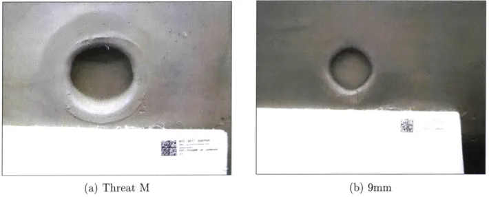
(a) Threat M (b) 9mm

Figure 1-2: Final clay deformation of clay from Threat M and 9mm impacts

simulations to be run on a large number of processors. In order to better understand the number of processors and the size of problem that could be effectively run, a scalability analysis was completed. The results are shown and discussed in Chapter 5, and provide insight into the parallel computing capability of the code with large problem sizes. The analysis of the scalability provides the ability to select the number of computation nodes optimal for a given problem size.

As part of the work with the cohesive zone model, the application of the framework to fragmentation of pressurized tanks was explored. In Chapter 6, a Saturn V helium tank simulation is discussed including the tank mesh, pressurization characteristics and fracture mechanics. The goal of the pressurized tank simulations is to generate a fragmentation catalog which can help determine how many fragments are created due a particular failure.

Chapter 2

Constitutive Model of Roma Plastilina

Clay

In order to model the drop test and high-velocity impact experiments, a model of the Roma-Plastilina clay is required. The model used for the clay is a variational Cam-clay theory of plasticity by Ortiz and Pandolfi, which is a variation of the original Cam-clay theory by Scholfield and Worth

[10,

20]. The main concepts are derived from observations of soil in laboratory tests and is heavily based on a critical state in which the soil or clay can sustain plastic deformation at constant volume. The constitutive model is discussed in further detail in Section 2.1. While testing different configurations of the clay, it was found that the model did not accurately characterize the material with large ranges of impact velocities (i.e. strain rates). The material could be calibrated to a low strain rate but would act overly stiff for high strain rates or could be calibrated to high strain rates and act too soft for low strain rates. Due to this behavior, the Cam-clay theory is modified to have a power-law rate dependency replace the original linear rate dependency shown in Section 2.2. In Section 2.2, the convergence conditions for this modification, as well as the validation and testing, are also discussed to show consistency with the derivation.

2.1

Summary of Original Model Formulation

For this work, the variational Cam-clay theory of plasticity by Ortiz and Pandolfi is used to model the Roma Plastilina [10]. This theory, as mentioned above, is better suited to model the behavior of Roma Plastilina as compared to other models that rely heavily on metal plasticity theory. The formulation of the original variational Cam-clay theory of plasticity is highlighted below with the major equations. The full formulation, with derivation of the following equations, can be seen in the work by Ortiz and Pandolfi [101. The implementation of the original variational Cam-clay theory of plasticity into computational framework, as well as testing of the original theory can be seen in the work by Fronk [11].

2.1.1

Governing Equations

To begin, the main assumption in the governing equations is the multiplicative decomposition of the deformation gradient F given by Equation (2.1) where F' and FP are the elastic and plastic parts, respectively, of the deformation gradient.

F = FeFP (2.1)

Free Energy

Ortiz and Pandolfi assumed that the elasticity and the specific heat of the material are independent of the preconsolidation pressure leading to the free energy given by Equation

(2.2) where We is the elastic strain-energy and WP is the stored energy of cold work [10].

A(F, FP, T, q) = We(Ce, T) + WP(T, q, FP) (2.2)

Focusing on the elastic strain-energy, the volumetric and deviatoric responses are decoupled for simplification giving Equation (2.3) where J' is the Jacobian of the elastic deformation and Cedev is the deviatoric elastic right Cauchy-Green deformation tensor.

The volumetric and deviatoric components are given by Equations (2.4) and (2.5), respec-tively, where 0e is the elastic volumetric strain, K is the isothermal bulk modulus, aT is the thermal expansion coefficient, To is the reference absolute temperature, po is the mass density per unit undeformed volume, C, is the specific heat. For the deviatoric portion, A is the shear modulus and ee is the deviatoric portion of the logarithmic elastic strain.

K

T

W T) - [0' - 3acT(T - T₀)]2 + poC' T i - log (2.4)

2 TO

Wedev = ie|2 _(2.5)

Flow Rule

The flow rule for this theory is assumed to be the von Mises flow rule shown in Equation

(2.6) where EP is the effective plastic strain and M is a tensor which defines the direction of

plastic flow f21j.

FPFP-1 = APM (2.6)

Ortiz and Pandolfi discuss the defining characteristic of the Cam-clay theory being that M can be any symmetric tensor that satisfies the kinematic constraint in Equation (2.7) where a is the internal friction coefficient and Mdev is the deviatoric part of M

1101.

2 (trM)2 +-MAdev MAdev = 1 (2.7)

0Z 3

Rate-sensitivity law

The rate-sensitivity law is originally assumed to be a linear rate-sensitivity and is given by the dual kinetic potential in Equation (2.8) where 77 is a viscosity constant.

*b = f(P)2 (2.8)

2

2.1.2

Yield Criterion and Hardening Rule

Yield Criterion

The yield criterion is given by Equation (2.9) in which p is pressure, q is stress and a is the internal friction angle which is related to the friction angle

#

by Equation (2.10)

q2 + _q0a2(p _ PO)2 = 02 6 sin q

3 - sin

#

(2.9)

(2.10)

From the yield criterion, the yield surface is generated as shown in Figure 2-1.

q

PC

PO

A

P

Figure 2-1: Yield surface in the (p, q)-plane, preconsolidation pressure pc and geometrical interpretation of the internal friction coefficient a

Hardening Rule

The hardening rule for the Cam-clay constitutive model is used to characterize the mecha-nisms of compression and swelling in granular mediums. The hardening characteristics are

700 60000 600 ₅₀₀₀₀ 500 40000 400 300 20000

200 -Droptest Armor Impact

100

10000

00

0 0 0.002 0.004 0.006 0.008 0.01 0.012 02 00 01

Time [s] Time [sI

(a) Drop Test Strain Rate (b) High-Velocity Impact Strain Rate

Figure 2-2: Strain rate versus time of the two main test types analyzed in this work

W

0 012

determined by the normal consolidation relation given by Equation (2.11) where pref and

OP _ref are material constants.

(2.11) Pc = Pref sinh P

ref

The stored energy function corresponding to the normal consolidation relation is given by Equation (2.12) by integrating over the volumetric plastic strain, OP.

OP

WCP(OP) = Pref Oe cosh O 1

ref

(2.12)

2.2

Power Law Rate Dependence Modification

For the application of the work, the clay is tested over two largely different strain rates. The first strain rate is generated from the drop test experiment in which the ball is dropped at a velocity of approximately 6.3 m/s producing a maximum strain rate of approximately 600 1/s and then tapers down to 0 1/s as the ball is caught in the clay as seen in Figure 2-2a. The second strain rate is from the high-velocity impact tests, in which the clay is topped by the Dyneema plate and then impacted with either a 9mm or Threat M, the maximum strain rate is closer to 55000 1/s and then again tapering to 0 1/s as the bullet gets stopped and the plate separates from the clay as seen in Figure 2-2b.

With the linear rate-sensitivity, the clay is overly rate dependent at high strain rates

causing the material to be stiff. To improve the rate dependency, a power law rate dependence was implemented that allows for the ability to use one set of parameters over a wide span of strain rates. The dual kinetic potential for the power law rate-sensitivity is given by:

* CA =

+

- M(2.13)

M + I ep

where m is the rate-sensitivity exponent, eP is a reference plastic strain rate, and o-, is the yield stress which is calculated using the yield criterion. Using the derivation in Section 2.1, the rate-sensitivity term in the original formulation, Equation (2.8), can be replaced with the power law rate-sensitivity, Equation (2.13), directly. This results in a formulation that allows for more control in the strain rate dependency of the Cam-clay material compared to the original formulation.

2.2.1

Power Law Rate-Sensitivity Implementation and Testing

Convergence and Conditions

A Newton-Raphson iteration is used to solve for the incremental plastic strain Ad and

phase angle

#

as shown by Ortiz and Pandolfi

[10.

The first condition of the power law rate-sensitivity equation is the plastic strain can not be negative so that condition was added to the Newton-Raphson to ensure that at the end of each iteration the value of the plastic strain is positive. Once the power law rate-sensitivity replaced the linear rate-sensitivity equation, the stability of the calculation of the phase angle improved, but began to oscillate with various tests of material parameters. It was determined Newton-Raphson would solve for a particular phase angle with a small change in the angle, but as the incremental plastic strain converged, the phase angle would start to oscillate between angles that varied by a period or more. The same angle was being calculated, but the change in the angle was approximately 27r, leading to the Newton-Raphson not converging for the phase angle. For this reason, a condition was added to the Newton-Raphson that forces the angle to be between 0 and 27r. Once this was implemented, the Newton-Raphson converged to a solution for the incremental plastic strain and the phase angle.

Linear Rate Dependence Versus Power Law

- 50000 1/s-Power Law

200 - _--- 5000 _{500 1/s-Power Law}1/s-Power Law

- 50 1/s-Power Law - 5 1/s-Power Law -- 50000 1/s-Linear 150 - - 5000 1/s-Linear - - 500 1/s-Linear - - 50 1/s-Linear - - 5 1/s-Linear Lfl tf 100- 5 0-fI I I 0.000 0.025 0.050 0.075 0.100 0.125 0.150 0.175 Strain

Figure 2-4: Power Law rate-sensitivity overlaid with Linear rate-sensitivity with forced equiv-alence by setting r7 in the linear model to be equal to the calculated o-o. Various strain rates are shown to see that the rate dependency is equal for this comparison

material to equal o- from the power law rate-sensitivity material. Figure 2-4 illustrates that

by forcing this equivalence, the power law rate sensitivity overlays the linear rate sensitivity

leading to the understanding that the power law rate-sensitivity was implemented correctly. With the power law rate sensitivity successfully implemented, the compression test can be used to get an understanding of how the new parameters, m and e', impact the rate dependency or behavior of the Cam-clay under various loading rates. In Figure 2-5, the same set of parameters was analyzed while changing the m parameter to discern how the stress is impacted for various strain rates. As m increases, the dependence on the rate begins to reduce. With a large value of m the expectation is that there would be little to no dependence on the strain rate. Figure 2-5 illustrates that as m increases, the material for high strain rates begins to behave like the material at lower strain rates. This includes yielding earlier as well as hardening in the same way. Looking at the derivative of the power

100 102 -Error vs Iteration 10-6 -0 L 10-10 1012 -10-16 -2 4 6 Iteration # 8 10 12

Figure 2-3: Convergence of Newton Raphson while using Power Law rate-sensitivity

was used which involves compressing the material at the same rate in all three principle di-rections. The convergence at the quadrature point at a random point in time was collected to get a number of samples. This collection of samples gives insight into the overall convergence behavior of the Newton-Raphson. With the added conditions for the Newton-Raphson, the convergence of the iteration is quadratic as is expected for a Newton-Raphson scheme. The convergence is shown in Figure 2-3.

Validation and Testing

As discussed in the work by Fronk, a hydrostatic compression test was used to verify the implementation of the Cam-clay material [11]. The modification to use the power law rate-sensitivity does riot have experimental data to verify the implementation other than forcing the linear and power law rate-sensitivities to be equal by setting m and 0 to 1, which produces the same equation as long as o is equal to 71. Because o is calculated using the preconsolidation pressure and the internal friction, Tj was set in the linear rate-sensitivity

law rate-sensitivity, Equation (2.14), the power of 1/m produces this behavior because as m increases, the dependence on the inner term decreases.

o- g1 +- (2.14)

For the reference plastic strain rate, the impact on the behavior of the material can be illustrated using Figure 2-6, in which, m is held constant at 1 but ' is changed. As e is increased, the magnitude of the stress at higher strain rates decreases as the inner term of Equation (2.14) decreases. Based off the graphs in Figure 2-6, with a high value of a the stress will converge to the yield stress and maintain that stress as the strain continues to increase. The inner term of Equation (2.14) will approach 1 as e approaches infinity thus the stress approaches the yield stress, illustrating that the power law rate-sensitivity modification is correctly implemented.

60- 50- 40-0. 20- 1 0- 50- 40- 30- 20-10 - 0-Stress Vs Strain, M=1 - 0.5 - -50s -500 - Soo - 50000 0.000 0.025 0.050 0.075 0.100 0.125 0.150 0.175 Strain (a) m = 1 Stress Vs Strain, M=4 0.5 -so -50000 0.600 0.025 0.050 0.075 0.100 0.125 0.150 0.175 Strain (c) m = 4 Stress Vs Strain, M=2 - 05 -5 - so - 500 - 5000 -- 50000 0.000 0.025 0.050 0.075 0.100 0.125 0.150 0.175 Strain (b) m = 2 Stress Vs Strain, M=5 - 5 - 5 -500 -sooo 50000" 0.000 0.025 0.050 0.075 0.100 0.125 0.150 0.175 Strain (d) m = 5

Figure 2-5: Stress versus strain curves of various strain rates showing the model response for hydrostatic compression test subject to various rate-sensitivity exponents with a fixed reference plastic strain rate of 1.

3.5 -3.0 - 2.5- 2.0-2 1.5- 1.0- 0.5-0.0] 6- 5- 4- 3- 21 - 0-M

Stress Vs Strain, lel --- 05 -50 -50 - 5000 -50000 0.000 0.025 0.050 0.075 0.100 0.125 0.150 0.175 Strain (a) EP = 1e1

Stress Vs Strain, 1e3

60 5o- 40- 30- 20-10 - 0-40 30 20 10 0 50 40 Ii30 20 10 0 30 25- 20- ~15- 10-51 0

Stress Vs Strain, 1e2

- 0.5 -50 -500 -5000 0.000 0.025 0.050 0.075 0.100 0.125 0.150 0.175 Strain (b) P = 1e2

Stress Vs Strain, 1e4

0.000 0.025 0.050 0.075 0.100 0.125 0.150 0.175 0.000 0.025 0.050 0.075 0.100 0.125 0.150 0.175

Strain

(d) i" = 1e4

Figure 2-6: Stress versus strain curves of various strain rates showing the model response for hydrostatic compression test subject to various reference plastic strain rates with a fixed rate-sensitivity exponent of 1. 29 - 0.5 - 5 - 50 -500 -5000 - 50000 0.000 0.025 0.050 0.075 0.100 0.125 0.150 0.175 Strain (c) 0" = 1e3 - 0.5 -5 -50 -50 -0W0 -5000 -

Chapter 3

Computational Framework

To simulate and model the test protocols, a computational framework entitled SUMMIT, developed at MIT under the direction of Raul Radovitzky, was used. SUMMIT is a solid mechanics code that is focused on large-scale simulations for materials and structures. The capabilities of the framework, include but are not limited to, continuous and discontiuous Galerkin methods, multi-scale simulations, explicit dynamics and higher order methods

[22,

23, 24]. In addition, SUMMIT has a wide variety of constitutive models and the capability to

quickly add and test new materials. SUMMIT is also highly scalable, which will be further discussed in Chapter 5, which offers many benefits with highly complex problems. The major features of SUMMIT that are used for the test protocol simulations are discussed below and include the continuum mechanics formulation, the contact algorithm for the projectile, discontinuous Galerkin (DG) method, and the cohesive zone model used for fracture and separation.

3.1

Continuum Mechanics Formulation

The base mathematical formulation for modeling finite deformation is based off deformation of a material and the linear momentum balance equation. The deformation gradient F is the deformation in the current configuration to the reference configuration as shown in Equation (3.1) where Xj is the material point coordinates in the reference geometry, xi is the material point coordinates in the current configuration, and p(X, t) is the Lagrangian of

the displacement vector. In Equation (3.2), the governing equation of the linear momentum balance is given where po is the initial density, j5 is the acceleration, P is the first Piola-Kirchoff stress tensor and B is the force per unit mass subjected on the body.

F -

_ax.

-(~ (3.1)

-

axj

Poo

= VO .p +poB in BO (3.2)

The first Piola-Kirchhoff stress is determined from the relationship between the PK stress and the Cauchy stress, og, shown in Equation (3.3) where J is the Jacobian derived from the determinant of the deformation gradient.

Pij = JaijF- (3.3)

J = detF (3.4)

The weak form of Equation (3.2) can be determined by multiplying the equation by a test function Ph and integrating over the domain which produces Equation (3.5) which can be summed over each element in the finite element problem. Within Equation (3.5), T is the applied traction.

(Po~ -6Wh + Ph: Vo6p=h) dV

JP

. V

+

p B

6,Wd -VdIS (3.5)

This weak form is the basis for continuous Galerkin (CG) methods.

3.2

Contact Algorithm

In this work, high-velocity impacts are modeled and an efficient way of modeling the impactor is needed. The contact algorithm prevents interpentration of objects which come in contact and is used to determine the resulting contact forces. In addition, the contact algorithm allows the impactor to be modeled as a rigid body with mass, without the need of a meshed object. The contact algorithm is needed for the drop test simulations, as well as the

high-velocity impact simulations in Chapter 4. The contact algorithm was implemented in the initial work by Fronk and is summarized in Appendix B [11].

The most important parameter for the contact algorithm is the penalty parameter as discussed in Appendix B. For the application of this project, the penalty parameter is de-pendent on the problem (type of material and type of impactor) in which it is applied. For the radius of the sphere, the size of the impactor for a given experiment is used which produces the desired undeformable object to impact the various surfaces. For the penalty parameter, two different values are used. For the drop test simulations and the high-velocity impact simulations, discussed in Chapter 4, the penalty parameter used was 4x108 and

1x10", respectively.

3.3

Description of Fracture

-

Discontinuous Galerkin and

Cohesive Zone Model

3.3.1

Discontinuous Galerkin (DG) Formulation

Discontinuous Galerkin (DG) methods allow for discontinuities within the problem domain which is beneficial in problems where fracture may occur or separation of elements is needed. For the application of the helmet test protocol, the plate and clay need to be able to separate in order to act as they do in experiments. With a continuous Galerkin (CG) method, the two materials must remain in contact throughout the simulation. The elements are not allowed to separate because the formulation is purely continuous. This is not physical as in the experiments, the two materials act separately and are not permanently joined. Employing a

DG method for the helmet system allows for this separation between the clay and Dyneema

plate.

Another use of the DG method is to model the delamination and fracture within the plate during an impact. The plate used in the experiments has plies and shows some separation between the plies occurring when some plies displace further than others. With a detailed mesh, the damage to the plate can be shown using the DG method. The DG method would allow the impactor to penetrate the plate producing delamination between the plies.

To achieve separation, delamination, and fracture, an explicit-dynamics spatial DG for-mulation is used. The explicit-dynamics spatial DG forfor-mulation for non-linear solid dynamics is discussed in further detail in the work by Noels and Radovitzky but the main points of the formulation are highlighted below [23].

To get the weak form of the problem, the continuum equations are first stated in material form by Equations (3.6),(3.6) and (3.6) with p being the deformation mapping where po :

BO -+ R+ is the initial density, i is the partial differentiation with respect to time at a fixed X, B is a force per unit mass subjected to the body, P is the first Piola-Kirchhoff stress tensor, N is the unit surface normal to the reference configuration and the boundary surface

aBO is split into the Dirichlet portion 8DBO and the Neumann portion aNBO. To integrate the system, displacement and velocity initial conditions are needed.

po46=Vo-P+poB VtcT (3.6)

p=i VXEDBO Vt c T (3.7)

P.N=T VXE&NBO Vt E T (3.8)

To formulate the DG method for a large class of materials, a variational constitutive framework is needed. This framework is discussed in Section 2.1 and Appendix Section

A.1.1.

DG discretization

In the DG discretization, Noels and Radovitzky start by defining an admissable test function

6

h E X [ [231. Integration over the body in the reference configuration of Equation (3.6)

multiplied by the test function leads to a weak formulation which consists of finding (p E Xk

and Ph E Sk such that Equation (3.9) holds 123].

(po45h - VO - Ph) - 6phdV = j poB6WhdV V6ph E Xk Vt

c

T (3.9)

With Equation (3.8) and the test function, the divergence theorem can be applied to produce Equation (3.10).

Ze fOe (POh * 6Wh + Ph : V6(Ph)dV - Ze N Ph - 6PhdS

=Ze fN hdS + Z poB -6WhdV V6Ph E Xk Vt c T (3.10)

The term on the interior boundary (1Q' may include fields that are discontiuous and therefore can have different values on either side of a surface. This is a defining characteristic of DG methods which address this problem with the concept of numerical flux. A full description of numerical flux is given in the work by Noels and Radovitzky

[23].

Including numerical flux in Equation (3.9), the weak formulation simplifies to Equation (3.11) where the jump ,[Oe] = 9+ - .- , and mean ,(o) = [++ *-], operators are defined on the space of the trace

of functions which can adopt multiple values on the interior boundary.

.(p (P h h + Ph : Vo0e(h)dV - f'e 6_{Ph (Ph) . N-dS}

T.6phdS +

J

2 poB - 6(PhdV V6ph

cXk

Vt E T (3.11)

In Equation (3.11), it is assumed that the constitutive law is enforced strongly from the compatible deformation gradient, Fh = VOph. Also, the displacement compability must be weakly enforced aiding in numerical stability. To do this, a quadratic stabilization term in

I[ b,

[

6 PbJ is used. For non-linear mechanics, the terms must be proportional to

[owh]

0 N- : C :

[Wh]

0 N- where C is the tangent moduli of the material. Using this term,

the displacement jumps are stabilized in the numerical solution, and the material relations at large displacements are considered. The final formulation consists of finding Ph E such that Equation (3.12) holds where h, is the element size and 3 > 0 is the stabilization

parameter.

IBOh PoPh 64h + Ph: V06(PhdV + f&B [PhJ (Ph) . N-dS

4-fBBh h

(9

N- : ((C) : [Ph] 0 N-dS

3.3.2

Cohesive Zone Model

For simulation the lose of material strength during fracture, a cohesive zone model is utilized.

A cohesive zone model for fracture is based off the idea of considering fracture as a process of

separation in material close to the tip of a forming crack

[15].

In order to model the gradual decline in the strength of a material as the elements separate a Traction Separation Law

(TSL) is used. The formulation used within SUMMIT and for this project is an extrinsic

approach with a linear irreversible softening law [15, 24, 251. This model works well for ma-terials that exhibit initially rigid response along the fracture surfaces. Due to the low strain failure of the Dyneema, as well as the brittle behavior of the matrix material, the extrinsic approach is reasonable for the application. The linear irreversible softening law is one of the most widely-used extrinsic cohesive laws and was originally proposed by Camacho and Ortiz [25]. The formulation of this approach is summarized below based off the formulation in Seagraves and Radovtizky work [151 and is tested using a bar spall simulation.

Formulation

The cohesive zone model is based on the use of the TSL. The TSL becomes active when the criterion in Equation (3.13) is satisfied where a, and at are the normal and tangential stress, respectively, 0 represents the ratio of G1Ic/G,, and oc is the critical effective cohesive strength.

ac O <; 2 + 7-t (3.13)

Once the traction separation law is initiated, the effective separation 6 in Equation (3.14), is used to determine the effective cohesive traction, Equation (3.15). In Equation (3.14), A,, and At are normal and tangential component of the separation.

5 =

t

+An (3.14)

T = 'o6,q (3.15)

86

In Equation (3.15),

#(6,

q) is the free energy density. For the particular case of the linear

3 0.2 0.4 0.6 1.2 1 0.8 TWOy. 0.6 0.4 0.2 0 0.8 1 1.2

Figure 3-1: T-6 relationship for the linear decreasing extrinsic law [15]

omax is the largest separation the crack experiences before closure or the current size of the

crack as it grows. In Equation (3.16), 6, is the separation where complete decohesion (T = 0) occurs and Tmax is the effective traction at 6 = 6

max Figure 3-1 depicts the relationship

between T and 6 as the traction separation law progresses based off Equation (3.16).

ac 1 - ) for

I

T-6 for < 6 max 6 > 0, 6 = 6max 0, or 6 < 6max

The total work of separation for the linear softening law is:

1

sep = U (3.17)

which is directly related to the Griffith critical energy release rate.

Bar Spall Test

The cohesive zone model shown above was tested with a simple bar spall test. The bar spall test was utilized in the work by Radovitzky et al. [24] to validate the discontinuous Galerkin and cohesive element behavior. This spall test was implemented in SUMMIT to confirm no errors existed in the prior implementation of the cohesive zone model. The bar spall consists of a rod of Neohookean material subjected to a tensile wave created by applying a normal

0.2 0.4. 0.6

6max 616C

T(6,6max) = (3.16)

15- 4

Figure 3-2: Structured 3D Mesh for Bar Spall test with 480 elements

velocity at each end of the bar. For the bar spall test shown here, the velocity oil the ends of the rod is 6.046 m s-'. The Neohookean material is defined by a Young's Modulus of 260 GPa and a Poisson's Ratio of 0 with a density of 3690kg/m3. The necessary cohesive parameters

are the Griffith critical energy release rate and the critical stress from which the critical separation can be calculated using Equation (3.17). The Griffith critical energy release rate is 34 J/M2 and the critical stress is 360 MPa giving a critical separation of 0.188 Pm.

Using the above material parameters, the bar spall simulation is set up using the mesh shown in Figure 3-2. Applying the velocity to each end, the tension wave propagates to the center then the two waves combine, making a stress high enough to create fracture as can be seen in Figure 3-3b. The displacement also becomes constant in the two halves as the separation has occurred as seen in Figure3-3a. Based off the results of the bar spall test, the implementation is correct and verified.

Kt N~~KKNKK4~N'ttKVtN1

I

-

-.

I'

71K 777TTij

(a) Displacement in the x direction (b) a-, stress

Figure 3-3: Left: X-displacernent as the velocity is applied at the time, velocity progresses toward the center of bar until frac occurs then both sides separate. Right: Stress in the x-direction shows a wave propagate towards the center, create fracture and then reflect until it dissipates. The final images have increased displacement to illustrate successful fracture.

-0 -IN

Chapter 4

Model Calibration and Results

Using the material constitutive models for the Roma Plastilina clay and the Dyneema plate, discussed in Chapter 2 and Appendix A, respectively, the experimental tests are simulated and the material models are calibrated to obtain results that are within the desired range of the experimental tests. There are three tests that are used to calibrate the material. The first is a drop test which is characterized as a low strain rate test. This experiment is originally used to make sure that the clay is conditioned properly prior to high-velocity impact tests and has set bounded that determine if the clay is conditioned properly or not. This test is discussed in Section 4.1 and is used to help provide more information about the clay behavior under an impact. Using the parameters obtained from the drop test experiment, the next two tests are both high strain rate simulations as they involve high-velocity projectiles. The first test is a high-velocity impact with a 9mm projectile and the second is an unknown projectile called Threat M. The tests and material calibration for these two threats are discussed in Section 4.2. The high-velocity projectile tests have a slight added complexity as there is an plate plate on top of the plate which absorbed the majority of the impact from the projectiles. To reduce the number of variables in the calibration, a set of Dyneema parameters were selected as discussed in Section 4.2.2.

To determine a starting point for the material calibration, literature on the characteri-zation of Roma Plastilina or modeling clay was used [9, 8, 6, 5, 71. The work by Hernandez focused on low strain rates associated with drop test experiments [6, 5, 7]. Hernandez's work on clay did not have a large range of strain rates, but the work from Buchely offered the

Experimental Drop Tnst Simulated Drop Test

Impact.,r o int. pn P atc '. velocy .10 m

rs eocy Of 6 261 m/s

0.mCkay Bl k I.nn Clay wm*c

a X5m, 0.305j

Figure 4-1: Left: Experimental Drop Test set up with impactor dropped from 2 m, Right: Simulation Drop Test set up with sphere impactor positioned at top surface of clay and given a kinetic energy equal to the potential energy at 2 m

largest range of strain rates (2300/s to 17,900/s)

[8].

Buchely provided information about how the material parameters may change at higher strain rates. For the Young's Modulus, a range of 1.73 MPa to 11.64 MPa was observed for the Roma Plastilina while the yield stress was between 0.08 MPa and 0.153 MPa and the Poisson's ratio was observed at 0.43

[8]. Based on the goal of finding a single parameter set for the clay material, in this work, the

ranges of parameters from literature were used as a starting point. However, with different model formulations, the material parameters proposed by Buchely were slightly deviated from the values when calibrating in SUMMIT. The following sections discuss the process of obtaining one parameter set for a variety of impacts.

4.1

Low Strain Rate

-

Drop Test Simulations

4.1.1

Mesh and Impactor

The drop test simulation is used to calibrate the clay parameters. The drop test, used by the Army Research Laboratory (ARL) for verifying the clay is well conditioned for high-velocity impact experiments, consists of a clay block 0.305 m wide by 0.305 m long by 0.1 m high, impacted with a 1 kg impactor [261. The impactor is a cylinder with a hemisphere on the end impacting the top surface of the clay after being dropped from a height of two meters as shown in Figure 4-1.

To simulate the ARL drop test configuration, the setup is modified to reduce compu-tational time and impactor complexity. The simulated drop test uses a clay block with

- - -I

(b) Angled view of Clay Mesh with impactor

(a) Top view of Clay Mesh

Figure 4-2: Clay mesh for the drop test simulation, includes a clay box 0.305 in wide by

0.305 m long by 0.1 m high which consists of 263,000 tetrahedral elements

the same dimensions as the experimental clay block, however the simulation impactor is positioned on the surface of the clay. At this point, the simulation impactor is given a ve-locity based on the initial potential energy the impactor had at 2 m which corresponds to

6.261 m s-1. The impactor is modeled as a sphere due to the contact algorithm discussed in

Appendix B. A mesh of the impactor is not needed as the radius of 0.0225 m can be set as the contact radius. Using the contact algorithm, the impactor is a single point representing the sphere impactor. The upper cylindrical portion of the experimental impactor is ignored but is considered acceptable as discussed in Fronk's prior work [11].

The mesh for the drop test simulation is shown in Figure 4-2. The mesh contains approx-imately 263,000 tetrahedral elements. The mesh is refined at the impact point to accurately capture the clay response. During the impact the elements experience high distortion and us-ing smaller elements helps to mitigate the numerical instabilities leadus-ing to mesh refinement at the impact point [111. The outer region is not refined since there is little deformation or mesh distortion and has minimal impact on the clay indentation. The drop test simulations are run using continuous Galerkin elements preventing fracture or separation of elements.

Parameter Set E(MPa) p po(MPa) m a e_ Depth (mm) 1 20 0.4 1 2 10 100 26.8 2 20 0.4 1 2 13 200 26.6 3 20 0.4 1 2 15 300 26.0 4 15 0.4 1 2 10 100 27.3 5 20 0.4 1 30 20 100 26.4 6 20 0.4 1 5 15 100 26.2 7 20 0.4 0.1 2 35 100 25.1 8 5 0.4 1 2 12 100 26.1

Table 4.1: Cam-clay Parameter Sets that produce clay indentation with range of calibration for experimental drop tests with p = 1529 kg/m3, Vref = 0.75. The experimental drop test

depth is 25.4t2.5 mm

4.1.2

Results

In order for the drop test results to be deemed calibrated, the depth of the impact must be within the acceptable bounds of clay indentation between 22.9 mm and 27.9 mm as specified

by ARL. A clay specimen with an indentation depth measured within the acceptable bounds

is considered well-conditioned and can be used for the high-velocity impact experiments.

A variety of parameter sets that produce a clay indentation within the experimental

range mentioned above are determined. The parameter sets are shown in Table 4.1. Multiple parameter sets are used to allow for further refinement at higher strain rates (Section 4.2). In the Table 4.1 it is seen that a wide variety of parameters can produce the depth required to meet the ARL clay calibration criteria. Although only eight parameter sets are shown, roughly 70 different parameter sets were found which also fit within the range specified. The results shown here are a sampling of those parameter sets but focus on the parameter sets that will be shown in Sections 4.2 and 4.3.

In Figure 4-3, the final time step of the eight parameter sets of Table 4.1 are shown. Based on the images, the impactors enters the clay and pushes the clay to the side creating a bulge outside the impact point. Depending on the parameters, the bulge is more or less pronounced. As seen in Figure 4-3g a high internal friction angle reduces the build up of material around the impactor. The high internal friction angle increased the friction within the material preventing it from sliding leading to reduced bulging. It can also be seen in Figure 4-3e, that a high rate sensitivity exponent will lead a large amount of build up along the edge of the impact region. Based on the power law rate-sensitivity discussed in Section 2.2, a high rate sensitivity exponent lessens the rate dependence producing a constant stress