HAL Id: dumas-00725217
https://dumas.ccsd.cnrs.fr/dumas-00725217
Submitted on 24 Aug 2012HAL is a multi-disciplinary open access
archive for the deposit and dissemination of sci-entific research documents, whether they are pub-lished or not. The documents may come from teaching and research institutions in France or abroad, or from public or private research centers.
L’archive ouverte pluridisciplinaire HAL, est destinée au dépôt et à la diffusion de documents scientifiques de niveau recherche, publiés ou non, émanant des établissements d’enseignement et de recherche français ou étrangers, des laboratoires publics ou privés.
Congestion Control in the context of Machine Type
Communication in Long Term Evolution Networks: a
Dynamic Load Balancing Approach
Dalicia Bouallouche
To cite this version:
Dalicia Bouallouche. Congestion Control in the context of Machine Type Communication in Long Term Evolution Networks: a Dynamic Load Balancing Approach. Networking and Internet Architec-ture [cs.NI]. 2012. �dumas-00725217�
University of Rennes 1
Research Master in Computing Science, Network and Distributed Systems
Master Thesis internship report
Congestion Control in the context of Machine
Type Communication in Long Term Evolution
Networks: a Dynamic Load Balancing
Approach
Work done by:
Dalicia Bouallouche (daliciabouallouche@inria.fr ) Supervisors: Adlen Ksentini (adlen.ksentini@irisa.fr ) Yassine Hadjadj-Aoul (yassine.hadjadj-aoul@irisa.fr ) DIONYSOS TEAM
IRISA/INRIA RENNES BRETAGNE ATLANTIQUE RESEARCH CENTER
Abstract
Machine Type Communication (MTC) is the automatic exchange of information through a network, including devices or machines, without human intervention. MTC applications aim to endow the machine with intelligence, in order to automate everyday life process. Some of the more established application areas are: health care, city automation, smart energy, positioning and tracking, security and surveillance, etc. MTC devices are generally spread in a wide area and should communicate through widely deployed networks. LTE cellular networks are choosen to support MTC applications since they offer a large coverage, and they are all-IP networks. The benefits of such a deployment are for both MTC application (more opportunities) and LTE networks (more revenues). However, the deployment of MTC applications over LTE networks incurs many requirements and causes challenges. The most important of them is the problem of congestion which is the focus of our work. Indeed, when the huge number of the MTC devices communicate at the same time, congestion occurs in different nodes of the network. In the present work, we propose a dynamic Load balancing and admission control algorithm which deals with the congestion in LTE networks. We balance the load among MMEs (Mobility Management Entities) before moving to the admission control so as to avoid congestion at the core network nodes. Through our discrete event simulator that we developped in C++, we show the efficiency of our solution since we obtain good simulation results, with different traffic patterns.
Keywords: MTC, LTE, Queueing Theory, Congestion Control, Load Balancing, Admission Control.
Contents
1 Introduction . . . 5
2 General overview of M2M applications . . . 7
2.1 Overall operation of M2M applications . . . 7
2.2 M2M application features . . . 7
3 MTC applications leverage LTE networks . . . 8
3.1 Architecture and key elements of MTC applications over LTE net-works . . . 8
3.2 Traffic management for MTC applications over LTE networks . . 9
3.3 Classification of MTC applications in LTE applications . . . 11
3.4 Main issues of M2M applications . . . 11
3.5 Congestion in MTC over LTE networks . . . 12
3.6 Congestion Control in MTC over LTE networks : traffic reject ap-proaches . . . 13
4 Overview of Load Balancing approaches . . . 15
4.1 Benefits of load balancing . . . 16
4.2 Some general load balancing algorithms . . . 17
4.2.1 Static load balancing algorithms . . . 17
4.2.2 Dynamic load balancing algorithms . . . 18
4.3 Related works on Load balancing in LTE networks . . . 19
5 MME load balancing in LTE networks . . . 21
6 Our Approach: Dynamic MME Load Balancing and Admission Control (DMLB-AC) . . . 22
6.1 Introduction . . . 22
6.2 Computation of Congestion and Reject Probabilities . . . 23
6.2.1 Congestion Probability . . . 24
6.2.2 Reject Probability . . . 25
6.3 Dynamic MME Load Balancing and Admission Control (DMLB-AC) Algorithm . . . 25
7 Performance evaluation . . . 29
7.1 Simulation model . . . 29
7.2 Simulated network topology . . . 30
7.3 Simulation scenarios . . . 30
7.3.1 Uniform traffic . . . 31
7.3.2 Random traffic with Bursts . . . 37
8 Conclusion . . . 41
List of Figures
1 MTC network architecture. . . 9
2 EPS Bearer Service Architecture [43]. . . 11
3 Congestion areas in MTC applications over LTE networks. . . 13
4 LTE network with more than one MME . . . 16
5 Concept for MME load balancing [4]. . . 22
6 M/M/1/K State transition diagram. . . 23
7 Simple M/M/1/K queueing node. . . 23
8 An execution example of our DMLB-AC algorithm in the case of load balancing among MMEs(Probabilistic routing). . . 28
9 An execution example of our DMLB-AC algorithm in the case of signaling traffic rejection (Probabilistic rejection). . . 28
10 Queueing Network Example. . . 29
11 Network topology for our simulation. . . 30
12 The Queueing Network model of our topology of simulation. . . 31
13 The number of packets in different MME queues in our DMLB-AC algo-rithm (the case of uniform traffic). . . 32
14 Number of lost packets in different MMEs in our DMLB-AC algorithm (the case of uniform traffic). . . 32
15 The number of packets in different MME queues for drop tail queue and a round robin distribution of packets (the case of uniform traffic). . . 33
16 The number of signaling packets lost in different MME queues for drop tail queue and a Round Robin distribution of packets (the case of uniform traffic). . . 33
17 The number of signaling packets in different MME queues for drop tail queue and a random distribution of packets (the case of uniform traffic) . 33 18 The number of signaling packets lost in different MME queues for drop tail queue and a Random distribution of packets (the case of uniform traffic). 33 19 Congestion probabilities of MME 0 and MME 1 (the case of uniform traffic). 35 20 The MME 1 Queue length according to its congestion probabilities (the case of uniform traffic). . . 35
21 Congestion probabilities of MME 0 and MME 1, Reject Probability and number of rejected packets of eNodeB 1 (the case of uniform traffic). . . 36
22 Congestion probabilities of MME 0 and MME 1, Reject Probability and number of rejected packets of eNodeB 0 (the case of uniform traffic). . . 36
23 Congestion probabilities of MME 0 and MME 1, Reject Probability and number of rejected packets of eNodeB 2 (the case of uniform traffic). . . 36
24 The number of signaling packets in different MME queues in our DMLB-AC algorithm (the case of random traffic with bursts). . . 39 25 Number of signaling packets lost in different MMEs in our DMLB-AC
algorithm (the case of random traffic with bursts) . . . 39 26 The number of signaling packets in different MME queues for drop tail
queue and a round robin distribution of packets (the case of random traffic with bursts). . . 39 27 The number of signaling packets lost in different MME queues for drop
tail queue and a round robin distribution of packets (the case of random traffic with bursts) . . . 39 28 The number of signaling packets in different MME queues for drop tail
queue and a random distribution of packets (the case of random traffic with bursts) . . . 40 29 The number of signaling packets lost in different MME queues for drop
tail queue and a random distribution of packets (the case of random traffic with bursts) . . . 40 30 Congestion probabilities of MME 0 and MME 1 (the case of random traffic
with bursts) . . . 40 31 The MME 0 Queue length according to its congestion probabilities (the
case of random traffic with bursts) . . . 40 32 Congestion probabilities of MME 0 and MME 1, Reject Probability and
number of rejected packets of eNodeB 1 (the case of random traffic with bursts) . . . 41 33 Congestion probabilities of MME 0 and MME 1, Reject Probability and
number of rejected packets of eNodeB 0 (the case of random traffic with bursts) . . . 41 34 Congestion probabilities of MME 0 and MME 1, Reject Probability and
number of rejected packets of eNodeB 2 (the case of random traffic with bursts) . . . 41
1
Introduction
Machine-to-machine (M2M) communication, also called Machine Type Communication (MTC)1, is the automatic exchange of information between end devices such as machines,
vehicles or a control center, which do not necessarily need human intervention [33, 45, 38]. The communication between devices is done through wired or wireless systems.
M2M includes technologies like mobile smart sensors, actuators, embedded processors and mobile devices, to interact with a remote server or device, so as to take measurements and then making decisions, or to monitor some physical phenomenas, without (or with only limited) human intervention [50, 9]. The role of human is only to collect data.
M2M applications aim to bridge the intelligence in the machine by delegating tasks to them, in order to automate everyday life process. Some of the more established appli-cation areas are: positioning and tracking, health monitoring, security and surveillance, fleet management and logistics, point of sales, automation and monitoring, automotive telematics, asset management, etc [9, 10].
Over the last two decades, mobile networks have enabled dramatic advances and changes in telecommunications. Mobile operators have grown to dominate the industry, offering their subscribers a service set as rich as their wired competitors, plus mobility. LTE (Long Term Evolution) network is a 4G wireless broadband cellular network technol-ogy (the next-generation network beyond 3G) developed by the 3GPP (Third Generation Partnership Project), an industry trade group [2]. It is named "Long Term Evolution" because it represents the next step (4G) in a progression from GSM (Global System for Mobile Communications), a 2G standard, to UMTS (Universal Mobile Telecommu-nications Systems), the 3G technologies based upon GSM. LTE provides significantly increased downlink peak data rate of 100Mbits/s in a 20MHz downlink spectrum, and uplink peak data rate of 50Mbits/s in a 20MHz uplink spectrum, backwards compatibil-ity with existing GSM and UMTS technologies, reduced latency, and scalable bandwidth capacity [13].
Recently, standardization activities on MTC over cellular networks have been launched by 3GPP group (SA2 group) [13] the fact that wireless cellular networks offer different network technologies and can widely support a huge number of MTC devices. Current studies aims to make improvements on that side, by supplying necessary network enablers for MTC devices.
The deployment of MTC applications over wireless cellular networks incurs many re-quirements and causes challenges, namely: to support the huge number of devices, to prevent congestion, to handle heterogeneous traffic characteristics of devices, to give high reliability, autonomy of the device operations, etc.
1
The focus of this work is the problem of congestion in M2M applications over LTE networks. Congestion occurs when a considerable number of M2M devices send signaling or data messages at the same time, trying to access the network. The mobile network operations may be thus very impacted, and both MTC and non-MTC traffic could be affected.
In the present work, we propose a solution that deals with congestion at the core part of LTE network with M2M applications. We suppose the case where each eNodeB (Evolved RAN (Radio Access Network)) is connected to more than one MME (Mobility Management Entity), which gives us the possibility to balance the load (signaling pack-ets) among MMEs. The load balancing avoids the case where some MMEs are congested, while others remain under-utilized. Our approach includes two steps, the first consists of balancing the load between the MMEs as much as possible, in order to use the MMEs that are underloaded, and alleviate the load of congested MMEs. To do that, we propose a dynamic algorithm that uses a defined Congestion P robabilities to balance the load among MMEs, by a probabilistic routing strategy for MTC signaling traffic. Second, we do an admission control at the eNodeBs (radio part) if all MMEs are likely to be con-gested and the load balancing is no longer sufficient to avoid congestion. The goal of the admission control is to reduce the traffic, by a probabilistic reject of the signaling traffic according to a defined Reject P robabilities. The parameters of the load balancing and the admission control are defined by the MMEs (core network nodes) which monitors the congestion.
To simulate our proposed solution, we developped a discrete event simulator, based on C++. The develloped solution uses technical methods from performance evaluation which consist of Queueing Netwrok modeling. By using this kind of performance evaluation, we disregard the details, and we handle the aspects of a system that are essential to its behaviour (which is mathematically analysed). Through the obtained results, we proved that our solution gives the results that we had expected. Thus, it balances the load between MMEs and controls the signaling packets admission efficiently, in order to handle congestion and to avoid packet losses.
This report is organized as follows: Section 2 will be devoted for an overview of M2M applications, namely their features, requirements and properties. In section 3 we define the case of MTC applications over LTE networks and the architecture of this network, we describe how the traffic is managed across this network, we classify MTC applications in LTE networks, we emphasize the problem of congestion in the case of MTC applications over LTE networks, and then we present congestion control approaches in MTC over LTE networks that exist in the literature. In sections 4 and 5, we surround the load bal-ancing, its benefits, existing algorithms that handles the load balancing and some state of the art regarding the load balancing in LTE networks. In sections 6, we present a detailed description of our proposed Dynamic DMLB-AC (Dynamic MME Load Balanc-ing/Admission Control) algorithm. The proposed solution is then evaluated in section 7 through simulations and discussions on the results. Finally, we conclude this report in section 8.
2
General overview of M2M applications
2.1
Overall operation of M2M applications
For every M2M application, there are four common basic stages of communication [9, 20]:
1. Collection of data: the process of M2M communication begins with capturing an event or taking data (temperature, inventory level, etc) using a device (sensor, meter, etc), and then converting it to digital data so that it can be analyzed and sent over a network, using IP packets.
2. Transmission of selected data through a communication network: the data is sent through a network to an application called a server, or to another device. There are several good options for transporting data from the remote equipment to the network operation center, like cellular network, telephone lines, and communica-tion satellites. Nevertheless, M2M applicacommunica-tions are mainly deployed over cellular networks, the reason that these later have widespread coverage.
3. Assessment of the data: when the application receives the data, it translates it into meaningful information (data stored, threats detected, etc) [1, 17], in order to be used in practical cases.
4. Response to the available information: after receiving and treating the data, the application (server or device) could send back an answer to the device.
2.2
M2M application features
The requirements of M2M communications are different from H2H (Human-to-Human, e.g. SMS, MMS) or S2H (Service-to-Human, e.g. downloading, streaming) ones, due to the difference between their nature of communications. Indeed, M2M communications are characterized by some features [9, 33, 34] mentioned below:
• Low devices mobility: devices do not move, move infrequently or move in a limited area.
• Large number of devices: a lot of close devices are required for typical applications to achieve high density, or distant ones for a large spread.
• Group based MTC features: devices may be grouped into groups, and each device may be associated with one group. It is interesting for multicast, policing and charging.
• Reduce costs: as these applications are used in everyday life, and may involve a large number of devices.
• Online small data transmission: MTC devices frequently send or receive small amounts of data.
• Time tolerant: data transfer can be usually delayed, except in some PAM cases. • Prior Alarm Messages (PAM): sending messages when immediate attention is needed,
in the case of theft, for instance.
• Secure connection: security exchange between devices and server.
• Packet Switched (PS) only: network operator shall provide PS service with or with-out an MSISDN (stand for Mobile Subscriber Integrated Services Digital Network Number, which is simply a telephone number of a SIM Card in a mobile/cellular phone).
• Location specific trigger: triggering MTC device in a particular area, e.g. wake up the device.
3
MTC applications leverage LTE networks
MTC applications have some technical requirements, among them, mobility, high data rates, efficiently sending signaling and data from devices to servers, etc. Mobile Network Operators (MNO) (like LTE networks) have already an expanded coverage deployed in-frastructure, and can withstand these requirements by carrying the data exchanged be-tween remote devices and servers for MTC applications [9, 17, 24, 12, 47]. It is very benefic for M2M applications to find an already and widely deployed infrastructure, with rich services, avoiding, thus, a cost of deploying a dedicated one. But it also offers plethora of revenue opportunities, in fact, M2M ecosystem (devices and services) is un-doubtedly the second highest revenue generating area for the MNO after mobile handset ecosystem [9, 37].
3GPP drives to simplify the previous 2G and 3G architectures behind the LTE project to define an all-IP packet only core network called the EPC (Evolved Packet Core net-work), which means that all packets crossing over this network are IP packets. In the case where MTC applications are integrated in LTE networks, traffic is splitted into sig-naling, which is the message that a UE (User Equipment) sends for a network connection request, and data is the useful message that a UE sends to the application [9, 32, 46]. Furthermore, LTE architecture is a fully meshed approach with tunneling mechanism over IP transport network [11].
3.1
Architecture and key elements of MTC applications over LTE
networks
The general architecture of M2M application over LTE networks is illustrated in Figure 1, which includes the following components [33, 9]:
• M2M device: referred to as UEs (User Equipments), capable on capturing events and data, and then transmitting them autonomously, or replying to requests for data contained within those devices.
• M2M gateways: they ensure M2M devices interconnection and inter-working to the communication network, using M2M capabilities.
• M2M device domain (M2M area network): it supplies M2M connectivity between M2M devices and Gateways.
• M2M Network domain (M2M communication networks): provides communication between M2M Gateways and M2M applications, e.g. xDSN, WLAN, LTE, WiMax, etc.
• M2M application: it is the destination of a data sent by a device over a network. It is used by the specific business-processing engines, e.g. M2M server, client application, etc.
Figure 1: MTC network architecture.
Table 1, defines the most important nodes in the EPC.
3.2
Traffic management for MTC applications over LTE networks
MTC communications in LTE networks use bearers (or tunnels) for messages sending. A bearer is established by the MME. It is created for a bidirectional IP traffic routing between devices (or UEs in LTE networks) and P-GWs, with a defined QoS (Quality of Service), especially just data and not signaling. Multiple bearers could be established for an UE so as to supply different QoS streams or connectivity to different PDNs. It should also across different interfaces to achieve the P-GW. Figure 2 shows the general scheme of the LTE bearer model.
Table 1: EPC’s most important nodes.
Node Description.
eNodeB Evolved RAN (Radio Access Network), sophisticated version of LTE base station.
P-GW Packet Data Node Gateway. It is responsible of allocating IP ad-dresses for UEs, and acts as the interface between the LTE net-work and external packet data netnet-works, by being the point of exit and entry of the traffic for the UE. An UE may have simultane-ous connectivity with more than one P-GW for accessing multiple PDNs. P-GW manages QoS (Quality of Service) and provides deep packet inspection, it also performs packet filtering for each user, sharing support, policy enforcement, and packet screening. More-over, the key role of the P-GW is to act as the anchor for mobility between 3GPP and non-3GPP technologies such as WiMax and 3GPP2 (CDMA1X and EvDo).
S-GW Serving Gateway. it routes and forwards user data packets, while also acting as the mobility anchor point for inter eNodeB handovers and as the anchor for interworking between 3G and LTE network. It also manages and stores UE information context, and holds data of downlink bearers when UE is in idle state (e.g. turned off for saving power, etc) and while the MME re-establishes the bearer with the UE.
MME Mobility Management Entity. It is the key control-node for the LTE access-network. It states, authenticates (by interacting with HSS) and tracks a user across the network. It is also involved in the bearer activation/deactivation process and it assumes functions related to attachment and connection management (authentication and establishing connection and security between the network and the UE). Moreover, it helps to reduce the overhead in the radio network by holding information about UEs. These functions are handled by the Session Management Layer in the Non-Access Stra-tum (NAS) protocol [9].
HSS The Home Subscriber Server. It contains subscription data users. It also holds the PDN to which user can connect as well as dynamic information such as MME to which the user is currently attached or registered.
MTC-IWF MTC Interworking Function hides the internal PLMN (Public Land Mobile Network) topology and relays or translates signaling proto-cols used over MTCsp to invoke specific functionality in the PLMN.
Figure 2: EPS Bearer Service Architecture [43].
3.3
Classification of MTC applications in LTE applications
To simplify the M2M application study, a classification is required. M2M applications are divided into three main classes according to the traffic and its origin, matching with data reporting way in Wireless Sensor Networks [31]. These three classes are:
1. Event driven applications: these applications have more priority than the rest. Indeed, each time an event occurs in the MTC device area, the UEs send messages to the server after being attached to the network, to inform about the event which can be with major importance, for example cardiac arrest in the case of health home monitoring irregular heartbeats or cardiac arrhythmia of a person. While no event occurs, MTC devices are detached from the network all the rest of the time, and remain in idle state.
2. Query driven applications: in this kind of applications, the MTC devices attach-ments to the network are triggered by a remote MTC server device which sends requests to these MTC devices. Hence, MTC devices can send data after being attached to the network. This is like a pull based application model.
3. Time driven applications: they follow the Event driven applications principle, but in this case, MTC devices send data periodically, every hour for instance.
3.4
Main issues of M2M applications
It is revealed through an analysis of M2M requirements that the challenges of M2M communications arise mainly from the following requirements [26]:
• Support for very high number of devices per cell:
- To be able to identify all devices. Addressing schemes have to be able to support all these devices.
- While preventing the congestion due to all the devices that are attempting to access the core network at the same time by sending messages signaling. It is the main study of this internship.
• These devices have varied traffic characteristics (delay tolerance, duty cycle, etc) of M2M communications, making them difficult to find a "one-size-fits-all" and regular transmission intervals solutions for access network and core network operation. • Low latency and high reliability.
• Some of these devices will be constrained in terms of power and storage. Thus, they require targeted solutions for achieving ultra-low power consumption.
• Support for different mobility profiles.
• The devices should provide autonomous operations, i.e. maintenance and configu-ration should be human free.
• The requirement that M2M communications must not negatively affect normal operation networks (H2H communications).
• Preventing physical attacks to unmanned devices, compromised (malicious or not) device behavior.
3.5
Congestion in MTC over LTE networks
One of the challenges a cellular network has to deal with is the congestion caused by large numbers of MTC applications. An important number of devices deployed in a small area, communicate frequently or infrequently by small amounts of data, trying to connect to the network, or to send data at the same time, by sharing the same nodes of the network (eNodeBs, MME, S-GW, P-GW, HSS), this obviously leads to congestion. It can also penalize non-M2M devices.
Two main types of LTE network congestion in the context of MTC applications could happen depending on where it occurs [9, 18, 5]:
• Radio network congestion: it happens when a high number of MTC devices are trying almost simultaneously to connect to the network, or to activate, modify and deactivate a connection. It frequently takes place in eNodeBs. More precisely, a lot of devices use the same channels, trying to connect to the same eNodeB.
• Core network congestion: it is congestion that occurs at the EPC part, may be caused by the simultaneous transmissions from a large group of MTC devices at-taches, to different cells. It appears in the MME (and hence HSS if a lot of devices have registered to the same HSS), S-GW, and P-GW.
These types of congestion are shown in figure 3.
Congestion due to user data packets is of less importance for this moment, thanks to the LTE-advanced radio technologies and LTE’s wide bandwidth. Indeed, 3GPP concentrates mainly on finding effective mechanisms and terms in order to manage congestion caused by lot of signaling messages coming from several MTC devices.
Figure 3: Congestion areas in MTC applications over LTE networks.
3.6
Congestion Control in MTC over LTE networks : traffic
re-ject approaches
Recently, some congestion avoidance schemes in LTE networks in the context of MTC application have been proposed. Two categorical classes are distinguished:
1. Soft mechanisms: in this category, the mobile operator seeks to minimize the fre-quency of MTC device attempts using soft measures, in order to carry out a par-ticular procedure without having to throttle them. Some solutions under this head are:
• Triggering MTC devices: the attachment of devices to the network is allowed if the MTC application or server sends alerts to the concerned devices, through the network. It is called a pull model. This can be done under the constraint that devices are not mobile (the location is known by the application).
• Reducing Tracking Area Updates (TAUs) signaling: TAU is used by the device to notify the network about its current location within the network. But sometimes it is unnecessary in the case of MTC devices with low mobility feature. Therefore, they minimize this kind of signaling by increasing the TAU period timer, on completely disabling it for static MTC devices.
2. Rigid mechanisms: rigid measures are taken by the mobile network operator to dismiss MTC devices that attempt to connect to the network if these simultaneous connections lead to contention. The following approaches are implemented accor-dance with this category:
• The grouping of MTC devices: the aim is to form groups of devices based on features or metrics like low mobility, low priority access, online/offline small data transmission, etc. The core network (mainly HSS) should have informa-tions about the groups and devices that belong to a group. Regarding the
subscription, the group is appeared as a single entity. Signaling overhead can thus be reduced and the devices’ management is simplified in terms of traffic, policing and charging.
• Allocation of grant time, forbidden time and communication window: these periods (based on the HSS subscription of the device) define the times when devices are allowed or not to attach to the network. During the "grand time interval", MTC devices are authorized to connect to the network. In contrast to "forbidden time interval" where MTC device connection is not authorized. During the grant time interval, in some applications, MTC devices do not need to connect to the network all this time. Indeed, a short communication window, which is sufficient for accomplishing the objectives of the targeted applications, is assigned to the devices during the grant time interval.
• Randomization of access times of MTC devices over the communication win-dow: in order to reduce peaks in signaling and data traffic during short com-munication window (due to several network connection attempts of MTC de-vices), the start time of the different MTC devices communication windows are randomized and distributed over the grant time period.
• Connection request rejection: it is another approach to cope with signaling congestion. It is to reject MTC signaling traffic (of MTC devices) either at RAN (Radio Access Network) or MME. This rejection operation should not af-fect non-MTC traffic, but have to target only MTC traffic of MTC applications that are causing congestion. Two rejection sources can be distinguished:
– Rejection by the RAN: in this case, to trigger MTC control access for over-coming congestion caused by MTC applications, the MME sends a notifi-cation message to RAN nodes (according to a congestion status feedback from P-GWs and S-GWs) to inform them about MTC barring information (e.g. barring factor, MTC group to block barring time, etc). Also, RACH (Random Access Channel) resources can only support low and medium traffic load, hence, unsuitable for MTC traffic which generates a lot of sending data. In fact, the risk of collision increases for both MTC and non-MTC traffic. To treat this problem, the work in [11] proposes differ-ent alternatives to control MTC access at the RAN level:
∗ Separating RACH resources for MTC and non-MTC devices, to main-tain normal network access for non-MTC traffic and limit the amount of MTC traffic entering the network.
∗ To complete the precedent solution, they include dynamic allocation of RACH resources. Where RACH resources can be dynamically in-creased by the network for the benefit of MTC devices, in the con-straint that the network knows the period of time the MTC devices have to transmit.
∗ Using specific large Backoff window for MTC devices so as to disperse the access attempts from MTC devices in large time intervals in order to overcome the RACH resources contention with UEs, and increase the access probability for non-MTC traffic that have higher priority.
∗ ACB (Access Class Baring). This method aims to effectively minimize the probability of collision in the case of several transmissions at the same time in the same RACH resource. In fact, it broadcasts an ac-cess class factor p (which is a probability of acac-cess) to the UE/MTC devices. Each UE generates a random number n then decides locally whether it can be proceed to the random channel access. If this ran-dom number is equal to or greater than p, then access is barred for a mean access barring time duration.
∗ CAAC (Congestion-Aware Admission Control) [9]. It is similar to the former ACB but the difference is that: first, in CAAC, the reject prob-ability p is derived by EPC nodes (MME, S-GWs and P-GW) under congestion, whereas ACB have no instructions on how to compute the reject probability p. Second, MTC devices are grouped into groups according to their priority classes, and the probability p is assigned to each group. Finally, accepting or rejecting MTC traffic is done at the eNodeBs unlike in ACB where the decision is made at the UEs. – Rejection by the MME: its principle is that MME determines authorized
times for each MTC device, by mean of HSS which informs MME on grant and forbidden time intervals as part of MTC subscription, and communi-cates them through MTC server to the respective MTC devices. However, congestion may occur during authorized times, in this case, MTC devices are provided with back off times for a later access after their connection was rejected by the MEE, or a congestion control notification message is sent to them so as to reduce data transmission rate.
Our work consists of controling the congestion that occurs at different nodes of the LTE network. We particularly focus on controling congestion at the core network part (MMEs) in the case of LTE networks that have more than one MME for each eNodeB, as illustrated in figure 4. We deal with congestion in two steps. First, we balance the load as much as possible among MMEs to avoid that some MMEs are likely to be overloaded, while others remain underloaded. Second, if the load balancing among MMEs is no longer sufficient, we move to the admission control to redure the traffic at the radio part (eNodeBs).
4
Overview of Load Balancing approaches
Load balancing is an important element for the implementation of services brought to grow. Its basic principle is to distribute service requests (tasks) across a group of servers, in intelligent manner. For this, a process of redirecting the tasks depending on the occu-pancy state of servers is required.
Commonly, load balancing systems includes popular web sites, large Internet Relay Chat networks, high-bandwidth File Transfer Protocol sites, Network News Transfer Protocol (NNTP) servers, Domain Name System (DNS) servers [53] and also evolved to support databases. Indeed, network overloads as well as server and application failures often threaten the availability of these applications. Whereas, they are expected to provide
Figure 4: LTE network with more than one MME
hight performance, hight availability, secure and scalable solutions to support all appli-cations. Ressource utilization is often out of balance, resulting in the hight-performance ressources remain idle while the low-performance ressources being overloaded with re-quests. Hence, for overload, performance and availability problems, a load balancing mechanism is a powerfull technique and a widely adopted solution.
LTE network is a promising candidate for next generation wireless networks. But like GSM and WCDMA, it still has the problem of load unbalance [49]. Much research has been done to deal with the load unbalance problem, we will see some of them later.
4.1
Benefits of load balancing
Load balancing has many benefits and deals with various requirements that are becom-ing increasbecom-ingly important in networks. It is particularly essential for networks that are very busy, it is in fact difficult to determine the number of requests that will be issued to a server. Therefore, the gains are significant:
• Increased scalability, High performance, High availability and disaster recovery. • Having multiple servers handling many requests, and using a mechanism of load
balancing to detect and identify the server that has sufficient availability to receive the traffic improves response time services.
• Load balancing permits to continue ensuring the service which remains available to users even if a server experiences downtime, because the traffic will be routed to an other server, depending on its load, proximity, or health.
• Optimal utilization of servers.
4.2
Some general load balancing algorithms
The key feature of a load balancing process is its abaility to direct service requests intel-ligently to the most appropriate server. We will present various load balancing algorithms, based on different parameters. Load balancing algorithms are classified into two typical approaches, we have static load balancing algorithms and dynamic ones [40, 16, 54]:
4.2.1 Static load balancing algorithms
In static load balancing [40, 16], the performances of the processors and the decisions related to load balance are determined at the beginning of execution, when resource requirements are estimated. Then depending on the processors performances, the work load is distributed from the start by the master processor [15, 29]. Static load balancing methods are nonpreemptive, indeed, a task is always executed on the processor to which it is assigned [40, 16].
Static load balancing schemes aim to reduce the overall execution time of concurrent program while minimizing the communication delays. Their main drawback is that the selection of a host for process allocation cannot be change during the process execution to make changes in the system load, because it is made when the process is already created. We will see some types of static load balancing algorithms:
1. Round Robin algorithm
It is a simple algorithm that distributes processes evenly between all processors [40, 16]. Each new process is assigned to a new processor in round robin order. It means that the selection is performed in series and will be back to the first processor if the last one has been reached. The advantage of round robin algorithm is that it does not require inter-process communication, and with equal workload round robin algorithm is expected to work well [36, 52, 53].
2. Weighted Round Robin algorithm
It is an enhancement of round robin algorithm which takes the response-time as a weight. Indeed, response times for each processor (or server) are constantly mea-sured to determine which processor (server) will take the next process (or server). 3. Randomized algorithm
In Randomized algorithm the processors (or servers) are chosen randomly, they use random numbers generated based on a statistic distribution [36, 40, 16].
Round Robin and Randomized schemes are not expected to achieve good per-formance in general case, but for particular special purpose applications, both can attain the best performance among all load balancing algorithms, and they tend to work well when the number of processes (requests) are larger than the number of processors (servers) [29].
4. Central Manager algorithm
In this algorithm, a central processor selects a server (or processor) to be assigned a request (process) [40, 28]. When a request is sent (or a process is created), the chosen server is the least loaded one. Central load manager retrieves informations
each time the load on system load state changes. It, hence, allows the best decision for asigning the request (or the created process) because it makes load balancing decision based on the system load information.
This algorithm is expected to perform better than the parallel applications, es-pecially when dynamic activities are created by different servers. However, high degree of inter-process communication could make bottleneck state [40, 16]. 5. Threshold algorithm
The principle of this algorithm is that the processes are assigned locally to processors immediately at the time of their creation. Each processor keeps a private copy of the system’s load and one of three levels characterizes the load of a processor: underloaded, medium or overloaded. Two threshold parameters can be used to describe these levels: t_upper and t_under [40, 16]. So, we have:
• load < t_under ⇒ Under loaded. • t_under ≤ load ≤ t_upper ⇒ Medium. • load > t_upper ⇒ Overloaded
All processors ara initially considered to be under loaded. Each processor sends messages to all other processors as soon as its load state exceeds a load level limit (t_upper) regarding the new load state, so as that all processors regularly update their load to the actual load state of the entire system. The process is allocated locally by a processor when its local state is not overloaded. Otherwise, it allocates a remote under loaded processor.
Threshold algorithms leads to performance improvements. Indeed, they decrease the overhead of remote process allocation and the overhead of remote memory accesses, because threshold algorithms have low intrer-process communication and a large number of local process allocations [40, 16].
We also mention that when all remote processors are overloaded, the process is locally allocated even if the local processor is overloaded. Therefore, it is a drowback the fact that it increases the execution time of an application and causes significant disturbance in load balancing, because the load on the overloaded local processor which is selected can be much higher than on the other remote overloaded processors [40, 16].
4.2.2 Dynamic load balancing algorithms
With dynamic load balancing, changes are made to the distribution of work among servers (or processors) at runtime, they use recent load informations when making distri-bution decision [27, 55]. Dynamic load balancing algorithms differ from the static ones in the fact that they allocate processes dynamically when one of the processors becomes under loaded [51, 41, 22].
1. Central Queue Algorithm
In this algorithm [21, 54], unsatisfied requests and new activities are stored as a cyclic FIFO queue on the main server (host). When new activity arrives at the queue manager, it is inserted into the queue. And each time the queue manager
receives a request for an activity, the request is buffered until a new activity is available if there is no ready activity in the queue. Else it removes the first activity from the queue and sends it to the requester.
When unanswered requests are in the queue and a new activity arrives at the queue manager, this new activity is assigned to the first unanswered request.
The local load manager sends a request for a new activity to the central manager when a processor load falls under the threshold, and if a ready activity is found in the process-request queue, the central load manager answers the request immediatly, else it queues the request until a new activity arrives.
2. Local Queue Algorithm
Its principle idea is to, first, statically assign all new processes to processors, then when processors get underloaded (their load falls under the threshold), a host initi-ates a process migration [21]. When a local host gets under-loaded, a comparison between the minimal number of ready processes of the local load manager and the remote load manager occurs to decide for the process migration. Some of the running processes are transfered to the local host if the minimal number of ready processes of the remote load manager is greater than the minimal number of ready processes of the local load manager. [40, 54].
A good description of customized load balancing strategies for a network of worksta-tions can be found in [56]. More recently, Houle and al. [19] consider algorithms for static load balancing on trees, assuming that the total load is fixed.
4.3
Related works on Load balancing in LTE networks
There are several ways to do load balancing in LTE networks, some of them are: In [49], they develop a practical algorithm for load balancing among multi-cells in 3GPP LTE networks with heterogeneous services. Its purposes are the load balancing of index of services with QoS requirements and network utility of other services. 3GPP LTE down-link multi-cell network deals with heterogeneous QoS users requirements, namely CBR (Constant Bit Rate) and BE (Best Effort) services.
Here, load balancing which is realized through enforced handover, aims to achieve max-imum load balance index for CBR as well as utility function for BE users ( [49], page 2). This paper proposes a heuristic and practical realtime algorithm which could be ex-ecuted in a distributed manner with low overhead, and could solve this multi-objective optimization problem in a sequential manner [49]. Its objective is that, first, in response to varying network conditions, each eNodeB in the network makes handover decision quickly and independently 2, and second, to minimize the overhead of user status
infor-mation exchange for decision making at each eNodeB. They propose a framework that consists of three aspects: QoS-guarantee hybrid scheduling, QoS-aware handover and call admission control.
The first one consists of allocating ressources according to the rate requirements for CBR users before scheduling the remaining resources for BE users to maximize the network
2
3GPP LTE network has a flat network structure without a central controller. Unlike UMTS that has radio network controller (RNC)
utility, because BE users have less QoS requirements than CBR ones. They could use op-portunistic scheduling among all CBR users to achieve less ressource occupation for each CBP user, then the ressource allocation depending on the average bandwidth efficiency is conservative.
In the case of BE users, they use the proportional fair scheduling in which all BE users have the same log utility function.
For the QoS-aware handover, they define a CBR user load balancing gain that permits for the CBR user to switch from cell i to cell j. When many CBR users are about to change their serving cells at the same time (which may result in oscillation of handover), a cell i chooses the best CBR user that achieves the largest benefit by changing its serving cell. Similarly, for a BE user, they define a load balancing gain of BE users, and the BE user that the cell selects is the one that achieves the largest gain because of changing its serv-ing cell.
Finally, for the Call Admission Control, when a new CBR user enters the network, the condition of its admission to access a cell i is the availability of enough time-frequency resource to satisfy its QoS demand. However, for new BE user entering the network, there is no constraint on cell access.
Other researches deal with load balancing problem in LTE-linked packet switched net-works. They often do not take into account QoS requirements, and use only proportional fairness as the scheduling metric among competing users [49, 14, 48]. Hence, other works include the QoS requirements by proposing a weighted proportional fairness scheduling schemes [39, 25] to reflect the network reality where QoS is required. However, users’ QoS requirements cannot be strictly guaranteed by the weighting method.
A self-optimizing load balancing algorithm in LTE mobile communication system is proposed in [23]. Its objective is to further improve network efficiency by delivering additional performance gain. This is possible with the use of load balancing in LTE Self-Optimizing Networks (SON), where the parameter tuning is done automatically based on measurements. Here, the basic principle is to adjust the network control parameters in such a way that overloaded cells can offload the excess traffic to lowloaded adjacent cells, whenever available, with the purpose of achieving load balancing. This load bal-ancing algorithm reacts to peaks in load and distributes the load among neighbouring cells to achieve better performance [44]. It aims to find the optimum handover offset value between the overloaded cell and a possible target cell. This aims to reduce the load in the targeted cell by ensuring that the handed over users to the target cell will not be returned to the source cell.
In this algorithm (of the paper [23]), they first list all the potential Target eNodeBs (TeNB) for load balancing handover and collect RSRP (Reference Signal Received Power) measurements from UEs to potential TeNB. They group users corresponding to the best TeNB for load balancing in accordance with the difference between TeNB and SeNB (Serving eNB: the eNodeB that serves the previous cell) and obtain information from TeNB on available ressources. Then, they estimate a number of required PRBs (Phys-ical Resource Blocks) after load balancing handover for each user in the load balancing handover group. This is before applying the load balancing procedure.
of the handover offset, with respect to the number of possible load balancing handovers. Then, a predicted (virtual) cell load after handover is estimated for a given handover offset T and cell C from the list of the potential TeNB. If this predicted load is lower than a certain acceptable threshold at TeNB, load at SeNB is reduced by the amount generated by the users handed over with this offset and handover offset to this cell is adjusted to the T value. This is repeated until the handover offset T is smaller than the maximum alowed value, and the SeNB load is higher than acceptable value threshold. In short, the main goal of this algorithm is to find the optimum HO offset that allows the maximum number of users to change cell without any rejections by admission control mechanism at TeNB side. This is done by evaluating the load condition in a cell and the neighbouring cells, and then estimates the impact of changing the handover parameters in order to imporve the overall performance of the network [23].
5
MME load balancing in LTE networks
The MME load balancing is a functionnality that permits to direct the attach requests of UEs to an appropriate MME, it aims to distribute the traffic to the MMEs according to their respective capacities, so as to perform load balancing, particularly as LTE networks are planned for large deployments, like M2M applications deployment.
Very few works deals with functionnality in the case of LTE networks. The only works that exist are those of 3GPP. We have, first, the load balancing between MMEs, where each MME have a Weight Factor (WF) configured, which is also kown as relative MME capacity since it is typically set according to the capacity of the MME itself relative to other MME nodes within the same MME pool [4]. This WF is conveyed to eNodeBs associated with the MME via S1-AP (Application Protocol) messages (see [3]) during initial S1 setup. An eNodeB can communicate with multiple MMEs in a pool, and it decides, based on the WF, to select the MME that can be loaded with attach requests. In fact, the probability of the eNodeB selecting an MME is proportianal to its WF. As illustated in figure 5.
Second, the load rebalancing may be needed if an MME needs to be taken out of sevice, or if it feels overloaded. Load rebalancing is a way to simply move UE attaches that are registred to a particular MME to another MME within the MME pool. Indeed, when an MME has been overloaded and cannot handle anymore attach requests, it frees up some ressources, then it releases the S1 and RRC (Radio Ressource Control) connections of the UEs (in ECM-CONNECTED state: a session with an active S1 connection) towards the eNodeBs, while asking UE to perform a "load balancing TAU (Tracking Area Update)". This is transmitted to UEs by eNodeBs in a RRC message. One a UE gets this message, it sends a TAU message to the eNodeB, which in turn routes the TAU message to another active MME (selected via the MME selection function). Therefore, the MME that is overloaded can move calls to an active MME that is not overloaded, and this, after pulling the UE context of the overloaded MME (via the S10 interface that connects the two MMEs) [35, 7].
will populate GUMMEI 3 (Globally Unique Mobility Management Entity Identifier) to
the eNodeB in an RRC message. Then, the eNodeB sends a DNS query to obtain MME information, based on the GUMMEI, and forward the UE message to the selected MME. If this last is not responding, then the eNodeB may forward the call to the next available MME in the pool.
Figure 5: Concept for MME load balancing [4].
6
Our Approach: Dynamic MME Load Balancing and
Admission Control (DMLB-AC)
6.1
Introduction
Our proposed approach aims to, first, balance the traffic among MMEs, which will prevent the congestion of some MMEs while the under-utilization of others, and second, to reject the traffic if all MMEs are about to be congested.
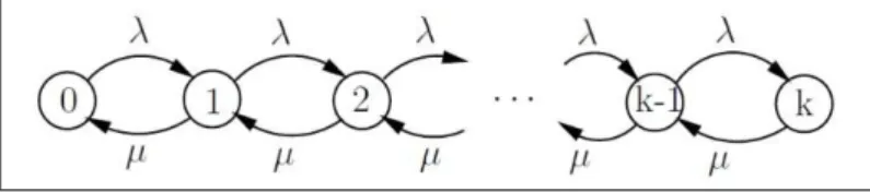
The congestion metric used in our approach is the queue length at the IP level. We estimate both Congestion and Reject rates respectively by Congestion Probabilities and Reject Probabilities at MMEs. To calculate these probabilities, we used a strong and wide modeling tool, namely: the Queueing Theory. Its analytical performance evaluation provides a mathematical basis that can help us for understanding and predicting the be-havior of our system, and getting its characteristics in order to describe its performances. Precisely, we use the M/M/1/K Queueing System which is appropriate to the MME be-haviour in our system. Indeed, the system has a single server, and a finite buffer (k-1 maximum waiting positions in the MME queue) with FIFO queueing discipline [30, 8, 6]. Figure 6 shows the state diagram for M/M/1/K queue model, and figure 7 illustrates a simple M/M/1/K queueing network.
In this queueing system, the packets arrive according to a Poisson process with rate λ (the mean number of packets that arrive per unit time), and the service time is Exponential of parameter µ. New coming packet is lost when he finds the system full.
In fact, at the origin, the traffic that a UE sends to the eNodeB do not follow a
pois-3
Globally Unique Mobility Management Entity Identifier. This consists of a Public Land Mobile Network (PLMN) identity, a Mobility Management Entity (MME) group identity and an MME code. The MME code is used in the eNodeB by the Non-Access Stratum (NAS) node selection function to select the MME.
son distribution. However, the agregation of all the trafic that UEs send is distributed according to a poisson process, with rate λ.
Figure 6: M/M/1/K State transition diagram.
Figure 7: Simple M/M/1/K queueing node.
The overall functioning of our Dynamic MME Load Balancing and Admission Control algorithm is as follows. At first, we aim to balance the load among all MMEs. This is achieved by performing the load balancing at the level of each eNodeB separately (we propose a distributed solution). The load balancing is handled by a probabilistic rout-ing strategy at each eNodeB that is connected to more than one MME, followrout-ing the inverseCongestionP robabilities of MMEs (after calculating the proprtions and the cu-mulative probabilities). The eNodeB retrieves these Congestion Probabilities from its MMEs. We also define a Congestion P robability threshold which is the limit that indi-cates us that the MME will be congested if more packets are forwarded to it.
When all MMEs are about to be congested, which means that there is no way to avoid congestion by balancing the load among MMEs, we move to the second step, which con-sists of the traffic rejection. Rejecting signaling traffic occurs when MME load balancing is no longer sufficient to deal with congesiton. It is done following the RejectP robabilities. It rejects the amout of traffic that can cause congestion, in order to maintain the number of packets in the MME queue much smaller than the maximum MME queue length. Rejecting traffic is done at the eNodeB that have triggered the rejection ((the one who was making the load balancing among its MMEs) as well as at the eNodeBs that share their single MMEs with the eNodeB that triggered the rejection, if they are believed to be the cause of congestion. In other terms, if an eNodeB have its Reject Probability higher than the Reject Probability of the eNodeB that triggered the rejection.
6.2
Computation of Congestion and Reject Probabilities
Analysis of queues requires defining some performance measures, and there are many possible measures of performance for queueing systems, and some of them are: probabil-ity of the number of customers in the system, probabilprobabil-ity of waiting for service, average
number of customers in the system, the average response time, the average waiting time, and the loss packet probability. But in our work, we are about to only use the proba-bility that there are n clients in the system, for estimating both Congestion and Reject probabilities. This probability is defined as follows (eq (1)) [30, 8]:
P (n) = ρn 1−ρ 1−ρk if n ≤ k and ρ 6= 1 1 k+1 if n ≤ k and ρ = 1 0 Otherwise (1) Such as: ρ = λ µ < ∞ The quantity ρ = λ
µ gives the system load, it is referred to as traf f ic intensity. For
M/M/c systems, there is a stability condistion ρ < c that simply shows that the system is stable if the work that is brought to the system is strictly smaller than the processing rate [30, 6]. However, in M/M/1/k the system is always stable, even if ρ ≥ 1, therefore, there is no stability condition [30, 8].
6.2.1 Congestion Probability
The Congestion Probability (eq (2) and(3)) is computed based on the formula (1). We recall that in our case, the congestion metric is the Queue Length. It means that the probability of congestion is the probability of having the number of packets (attach request) in the queue greater or equal a certain Queue Reference QRef. Hence, we define
the congestion probability as follows:
PCong = P (n ≥ Qref) = k−1
X
n=Qref
P (n) (2)
After replacing P (n) by its formula (eq (1)), we will have:
PCong = 1−ρ 1−ρk k−1 P n=Qref ρn if ρ 6= 1 k−Qref k+1 Otherwise (3)
For each MME, there can be more than one eNodeB. Thus, the flow (or traffic) entering the MME buffer, comes from all eNodeBs connected to it. So, we will have:
ρ = λ µ Such as : λ = nb_eN Bs X i=1 λi (4)
6.2.2 Reject Probability
The Reject Probability (eq (5) and (6)) is similarly defined as the Congestion Proba-bility. The only difference is in eq (4). So we have:
PRej = P (n ≥ Qref) = k−1 X n=Qref P (n) (5) PRej = 1−ρ 1−ρk k−1 P n=Qref ρn if ρ 6= 1 k−Qref k+1 Otherwise (6) ρ = λ µ (7)
The probability of Reject depends only on a single flow (λ of eq (7)), because we want to estimate the congestion regarding each eNodeB separately, and then reject the traffic following this probability, which is proportional to the number of packets (requests) sent by each eNodeB (more exactly proportional to λ).
Unlike the Reject Probability, the Congestion Probability depends on all the flows coming from all eNodeBs connected to the MME (eq (4)), because we want to estimate the congestion caused by the whole received traffic, in order to control it.
6.3
Dynamic MME Load Balancing and Admission Control
(DMLB-AC) Algorithm
Given an LTE network with n eNodeBs, and m MMEs. In the following, we define our DMLB-AC (Dynamic MME Load Balancing/Admission Control) algorithm:
1. Comments on our DMLB-AC Algorithm
When an eNodeB that is connected to more than one MME receives an attach request packet from a UE, we verify the number of MMEs that an eNodeB has. We do the Load Balancing only when an eNodeB has more than one MME. The Load Balancing is not possible if an eNodeB has just one MME.
We define a congestion probability threshold, that we set to 0.5. An MME that has PCongi[j] ≥ 0.5 means that this MME is getting congested. If there is at least
one MME that has PCongi[j] < 0.5, it means that at least one MME is not yet
con-gested, and can still receive traffic. So, we call the P robabilisticRouting(PCongi[])
procedure, with the Congestion Probabilities PCongi[] as a parameter.
Otherwise, when all MMEs of an eNodeB are getting congested, it means that a the load balancing by a probabilistic routing strategy in no longer sufficient. So, we have to call P robabilisticReject(PReji[]) procedure, with the Reject Probabilities
Algorithm 1 DMLB-AC Algorithm
1: Each eN Bi that is connected to more than one M M E requests
Congestion P robabilities (PCongi[j]) f rom its M M Es;
2: Each M M Ej sends its PCongi[j] to the eN Bi;
3: W hen eN Bi receives a packet (attach request) f rom a U E :
4: if (N b_M M Es_of _eN Bi > 1) then
5: if (∃ M M Ej : PCongi[j] < P congT hresh) then ⊲ P congT hresh is set to 0.5
6: −Call procedure : P robabilisticRouting(PCongi[]);
7: else
8: −eN Bi Requests Reject P robabilities (PReji[j]) f rom its M M Es;
9: −Each M M Ejsends the corresponding Reject P robabilities to the eN Biand
to each eN B that have a single M M E, and shares this M M E with the eN Bi;
10: −Call procedure : P robabilisticReject(PReji[]);
11: end if
12: else
13: −F orward the P acket(Request) to its singleM M E;
14: end if
Algorithm 2 Probabilistic Routing Procedure
1: procedure ProbabilisticRouting(PCongi[])
2: −let M the set of M M E indexes connected to eN Bi;
3: −Computation of inverse probabilities :
4:
5: ∀j ∈ M : P _IN VCongi[j] ← 1 − PCongi[j];
6: −Computation of proportions : 7:
8: ∀j ∈ M : PP ropi[j] ← PP _IN VCongi[j]
k∈M
P _IN VCongi[k];
9: −Computation of cumulative probabilities :
10:
11: PCumuli[0] ← PP ropi[0];
12: for j = 1 : card(M ) − 1 do ⊲ card(M ) is the cardinal number of the set M.
13: PCumuli[j] ← PCumuli[j − 1] + PP ropi[j];
14: end for
15: j ← 0;
16: k ← M.f irst_element();
17: unif ← random(0, 1);
18: while ((j < card(m)) and (unif > PCumuli[j])) do
19: j ← j + 1;
20: k ← M.next_element(); 21: end while
22: −F orward the P acket(Request) to the M M Ek;
2. Comments on the Probabilistic Routing Procedure
We balance the load in accordance with the inverse of the Congestion Probabil-ities or the probabilProbabil-ities that an MME is not getting congested. In other terms, we balance the load by forwarding the traffic according to the remaining capac-ity of the queue, without achieving congestion (or without exceeding the queue reference QRef). For instance, let PCong[1] = 0.2 and PCong[2] = 0.5 the
con-gestion probabilities of the M M E1 and the M M E2, respectively. The M M E2
has a greater probability to be congested than the M M E1. It means that, we
will forward (1 − PCong[1]) ∗ 100 = 80% of the eNodeB traffic to the M M E1 and
(1 − PCong[2]) ∗ 100 = 20% of the same eNodeB traffic to the M M E2.
With the computation of proportions, we seek to have well dispersed probabilities (with
m
P
i=1
PP rop[i] = 1). And the computation of the cumulative probabilities is
to avoid having two identical probabilities, in order to do a fair routing. These cumulative probabilities are those we use to perform the probabilistic routing at-tach request packets. The packet request is forwarded to the corresponding M M Ej
when unif < PCumul[j].
Algorithm 3 Probabilistic Reject Procedure
1: procedure ProbabilisticReject(PReji[])
2: unif ← random(0, 1);
3: if (unif ≤ M ax(PReji[])) then
4: −Reject the packet (attach request);
5: else
6: −Call procedure : P robabilisticRouting(PCongi[]);
7: end if
8: if ∃ j so that eN Bj have a single M M E, and shares this M M E with the eN Bi
9: if (PRejj > M ax(PReji[])) then
10: unif ← random(0, 1);
11: if (unif ≤ PRejj) then
12: −Reject the packet (attach request);
13: else
14: −F orward the packet to its single M M E 15: end if
16: end if
17: end procedure
3. Comments on the Probabilistic Reject Procedure
The eN odeBi (that triggered the rejection) receives the Reject Probabilities
(PReji[j]) from its MMEs. The signaling packet rejection will be done according to
the highest reject probability among the PReji[j].
Figure 8: An execution example of our DMLB-AC algorithm in the case of load balancing among MMEs(Probabilistic routing).
Figure 9: An execution example of our DMLB-AC algorithm in the case of signaling traffic rejection (Probabilistic rejection).
M ax(PReji[]) ∗ 100% is rejected.
We also test for each eN odeBj, which has a single MME and shares this MME
with the eN odeBi, whether it has a greater reject probability ((PRejj) than the the
highest reject probability of eN Bi (M ax(PReji[])). Which means that the eN odeBj
is the cause of congestion. If it is the case, eN odeBj shall make the admission
control and reject traffic at its level, because it is the one that generates the most traffic and causes congestion. We do not reject the traffic at the eNodeBs that have other MMEs (in addition to the one it shares with the eN odeBi that triggered the
rejection) since they (may be) can still balance the load at their levels.
An execution example of our DMLB-AC algorithm in the case of load balancing among MMEs(Probabilistic routing) and in the case of signaling traffic rejection (Probabilistic rejection) is illustrated in figures 8 and 9.
7
Performance evaluation
7.1
Simulation model
We evaluate the performnces of our solution using Queueing Network modeling, which is a technical approach of performance evaluation with a probabilistic approach, and we implement our simulator with C++ langage. Queueing Network modeling is used to approximate a real queueing situation or system, and the queueing behaviour can be mathematicaly analysed. Queueing Network is a very important application of Queueing Theory. It is a ’Network of Queues’ which is a collection of queues where customers (signaling and data packets in our case) are waiting for accessing a service station (which represent eNodeBs, MMEs, PGWs, and SGWs in our case), and the input from one queue is the output from one or more others.
We chose this kind of simulation because it is the most appropriate for our approach which is based on Queueing Theory and analytical approach of performance evaluation that we use for computing our needed metrics (Congestion and Reject Probabilities), and also because using a model to investigate system behavior is less laborious and more flexible than experimentation, because the model is an abstraction that avoids unnecessary detail. In fact, the Queueing Network model is an abstraction of a system, an attempt to distill, from the mass of details that is the system itself, exactly those aspects that are essential to the system’s behaviour. Once a model has been defined through this abstraction process, it can be parameterized to reflect any of the alternatives under study, and then evaluated to determine its behavior under this alternative.
An example of a Queueing Network in illustated in figure 10.
Figure 10: Queueing Network Example.
In our case, the eNodeBs queue type is M/M/1, because the duration between two arrivals and the service duration are exponential, and there is one service station (eNodeB) per queue, with infinite queue size.
The MMEs queue type is M/M/1/K because the duration between two arrivals and the service duration are exponential, there is one service station (MME) per queue, the queue
size is finite and its maximum capacity is K.
The output packets of eNodeBs are the input packets of the MME queues.
7.2
Simulated network topology
Figure 11: Network topology for our simulation.
Figure 11 illustrates the simulated network topology. We represent only the control plane links, and we do not represent other nodes (PGW, HSS, MTC-IWF, etc) because we deal with only signaling traffic, and we focus on congestion at the Core Network part, especially at the MME level. We are not interested in the Radio part. The goal of our work is to avoid congestion at MMEs and to treat it if it should appear.
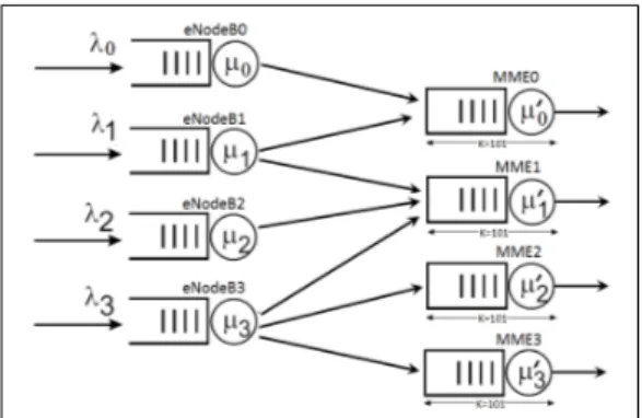
The Queueing Network model of our topology is illustrated in figure 12. We represent the eNodeBs by the four queues on the left of the figure. They are connected to different MMEs that we represent by the four queues on the right of the figure.
Our model contains only eNodeBs and MMEs because we deal with congestion due to signaling traffic which goes through eNodeBs and then MMEs. We recall again that the congestion metric that we take into account is the queue length, so a model with Network of Queues is sufficient to model the parts of the LTE network that we need, to approximate a real queueing situation or system, so as the queueing behaviour can be analysed mathematically, and to evaluate the performances of this model using usefull steady state performance measures, including the average number of packets (customers) in the system or in the queue, the average time spend in the system or in the queue, the probability to have the system in a certain state (that we use for evaluating the congestion and the reject probabilities), etc.
It is proved that analysis of the relevant queueing models allows the assessment of the impact of proposed changes and to identify the cause of queueing issues.
7.3
Simulation scenarios
In our tests, we consider traffic sent to the eNodeB by the UEs with rate λ packets/second, and then packets are sent to the MMEs with different rates (according to the congestion
Figure 12: The Queueing Network model of our topology of simulation.
rate of each MME) that we compute at runtime, and which will be then used to specify the congestion probabilities for each MME.
One of the specific characteristics of MTC applications is the bursty traffic it generates, since MTC devices are likely to send data at synchronized periods, like when an event occurs, or when the devices send packets periodically (timer fired). So, we test our approach in the case of bursty traf f ic scenario (which reflects reality), in the case of unif orm traf f ic which could also reflect a real scenario [42]. In fact, in a time driven application, nodes are scheduled in different intervals by synchronizing their sendings at the application level, in order to prevent bursts. And also in the case of random traf f ic to generalize the behaviour of the MTC applications in LTE networks in all cases that may occur.
We compare our proposed solution with two other methods: Random Distribution of packets which distributes packets without trying to balance the load between MMEs, and Round Robin Distribution of packets. These two approaches do not have any admission control (traffic rejection), and the queue of the MMEs is of type Drop Tail Queue (FiFo).
7.3.1 Uniform traffic
Here, we consider Uniform traffic scenario. Table 2 shows the parameters of the simula-tion. In this scenario, the attach requests generated by the UEs toward the eNodeBs are uniformly distributed over the time, so that there is no bursts.
Figure 13 shows the evolution of the queue length of all MMEs in the case of our proposed DMLB-AC algorithm. We note that the queue length of all MMEs are quite similar starting from the second period of simulation. This is due to the fact that we set, at the beginning, the Congestion Probabilities to 0, and starting from the second period, the new Congestion Probabilities are calculated and the traffic reacts according to them. In fact, our goal is to balance traffic between MMEs and to maintain, at each instant, almost the same number of packets in all MMEs, in order to prevent congestion at some MMEs and the under-utilization at others. This is done by our dynamic load


![Figure 5: Concept for MME load balancing [4].](https://thumb-eu.123doks.com/thumbv2/123doknet/6152766.157483/24.892.320.567.237.413/figure-concept-for-mme-load-balancing.webp)